Quasi-deterministic generation of maximally entangled states of
two mesoscopic atomic ensembles by adiabatic quantum feedback

Abstract

We introduce an efficient, quasi-deterministic scheme to generate maximally entangled states of two atomic ensembles. The scheme is based on quantum non-demolition measurements of total atomic populations and on adiabatic quantum feedback conditioned by the measurements outputs. The high efficiency of the scheme is tested and confirmed numerically for ideal photo-detection as well as in the presence of losses.

I Introduction

Quantum entanglement is one of the most fundamental aspects of quantum mechanics, as well as an essential resource in quantum communication and information processing. Although very difficult to realize, entangled states of material particles have been thoroughly studied in recent years both theoretically and experimentally, and some schemes for their generation have been designed and partially realized. Some studies concentrated on how to produce entanglement between groups of two or few atoms, exploiting for example the collective vibrational motion of trapped ions molmer99 ; sackett2000 , the single-photon interference at photodetectors cabrillo1999 , or the conditional dynamics of two atoms within a single-mode cavity field plenio1999 . More recently, there has been a growing interest on how to create multipartite entanglement between atoms belonging to a single atomic ensemble considered as a multi-party quantum system, by exploiting the interaction with a light field sorensen2001_1 , and the subsequent detection process duan2003 ; stockton2004 . Finally, and more ambitiously, various schemes have been proposed for the entanglement of different (two or more) macroscopic or mesoscopic atomic ensembles duan2000 ; juls01 ; duan2002 ; ADL3 ; sherson05 .

In the cases of several (at least and typically two) macroscopic atomic ensembles, where collective atomic operators can be described by some continuous-variable approximation, it is only possible to design schemes for the realization of weak entangled states. Some of these schemes exploit quantum non-demolition (QND) measurements on auxiliary electromagnetic fields (usually assumed in some Gaussian state) interacting with the atoms to prepare entangled states of atomic systems duan2000 ; juls01 ; ADL3 . However, the probabilistic nature of the quantum measurement events makes the generation of atomic entangled state conditioned by the measurement outcomes, usually yielding a low probability of success. This is particularly true for the preparation of maximally entangled states. Such a shortcoming should be in principle overcome by exploiting the knowledge of the state vector of the atomic system conditioned on the outcome of a measurement, and then by introducing a proper feedback scheme to efficiently drive the system toward a maximally entangled state. Actually, Stockton et al. showed in Ref. stockton2004 how this strategy can be properly used to deterministically prepare highly entangled Dicke states of a single atomic ensemble.

In the present work we introduce a reliable feedback scheme to generate maximal entanglement of two mesoscopic atomic ensembles. In this scheme, the discrete quantum nature of the atomic systems is fully taken into account without resorting to any continuous variable or Gaussian approximation. Our proposal is based on the model introduced by Di Lisi and Mølmer ADL3 , where two collections of atoms, probed by a sequence of single-photon scattering processes, are conditionally entangled by QND measurements of the total atomic population difference between the two atomic samples. This model has been recently shown to be robust against spontaneous scattering DLDSI04 .

In the present work the results of the QND measurements obtained by photo-detections are exploited to drive the system into the maximally entangled state by a suitable feedback mechanism. The feedback scheme that we introduce is a proper modification to the fully discrete case of the continuous feedback strategy originally designed by Thomsen, Mancini and Wiseman (TMW) TMW02 ) to generate high spin squeezing of a single atomic ensemble, whose experimental realization was recently obtained by Geremia et almabuchi . The same scheme was generalized to the case of two atomic ensembles to produce two-mode spin squeezing BerrySanders02 .

Our procedure is monitored by quantitative wave-function simulations which show how the sequence of photo-detection events, followed by the feedback signal, gradually modifies the state of the samples and post-selects the maximally entangled states. We show that the feedback scheme enormously increases the rate of success in producing maximally entangled states of the two atomic ensembles compared with the scheme in which feedback is absent. We also show that the efficiency is further improved by adiabatically switching off the feedback signal; in this way one obtains a quasi-deterministic generation of the maximally entangled state. Finally, we study the problem for the more realistic case of imperfect detectors, and we show how the feedback scheme guarantees a very high probability of success in this case as well, making the mechanism quite reliable against losses.

II The model

The two atomic ensembles, denoted by “$1$” and “$2$” respectively, are identical, and each one is constituted by $N$ identical atoms in a static magnetic field, whose level structure consists of two metastable lower states, $|g\rangle$ and $|f\rangle$, that correspond to Zeeman sublevels of the electronic ground state of alkali atoms, and one excited state $|e\rangle$, cf. Fig 1.

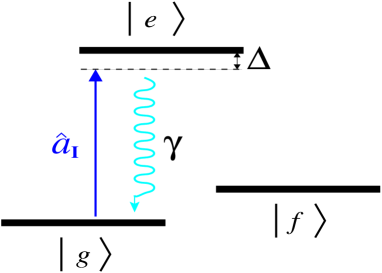
Figure 1: (Color online). Level structure of the atoms. $|g\rangle$ and $|f\rangle$ are metastable states, $|g\rangle$ is coupled off resonantly by the electromagnetic field, whose annihilation operator is $\hat{a}_{I}$, to the excited state $|e\rangle$. Here $\gamma$ is the spontaneous transition rate and $\Delta$ is the detuning between the coupling field and the atomic transition frequency.

We then consider an optical beam passing through the atomic clouds which is coupled (out of resonance, with detuning $\Delta$) only to the transition $|g\rangle\rightarrow|e\rangle$. We can introduce the atomic spin operators for an atom $a$ in ensemble $i$ as

$$j^{(i)}_{a,x} = \frac{|f\rangle_{a}\!\langle g|+|g\rangle_{a}\!\langle f|}{2}\;,$$

$$j^{(i)}_{a,y} = \frac{|f\rangle_{a}\!\langle g|-|g\rangle_{a}\!\langle f|}{2i}\;,$$

$$j^{(i)}_{a,z} = \frac{|f\rangle_{a}\!\langle f|-|g\rangle_{a}\!\langle g|}{2}\;.$$ (1)

where $a=1,...,N$ is the atomic index and $i=1,2$ is the ensemble index. The dynamics of the ensembles can be described by collective spin operators whose $x$-,$y$- and $z$-components, for each ensemble $i$, read

$$\hat{J}^{(i)}_{x}=\sum_{a=1}^{N}j^{(i)}_{a,x}\;,\;\;\hat{J}^{(i)}_{y}=\sum_{a=1}^{N}j^{(i)}_{a,y}\;,\;\;\hat{J}^{(i)}_{z}=\sum_{a=1}^{N}j^{(i)}_{a,z}\;.$$ (2)

These sums define the $x$-,$y$- and $z$-components of the collective angular momentum $\hat{J}^{(i)}$. In particular, the eigenvalues $m_{i}$ of $\hat{J}^{(i)}_{z}$ are proportional to the population difference in the two stable states.

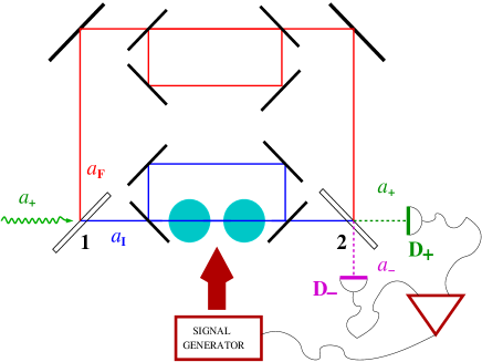
Figure 2: (Color online). Schematic experimental configuration. Atoms occupying the internal state $|g\rangle$ in the two samples interact with the light field, incident from the left. The presence of the cavities guarantees a high spectral and directional resolution of the entering photon. The phase shift of the light field due to the interaction with the atoms is registered by the different photocurrents in the two detectors. These signals can be combined with that produced by a signal generator and hence sent back to the two ensembles.

The two atomic ensembles are initially prepared, by optical pumping, so that each ensemble is fully polarized along the $x$-axis with collective spin equal to $J^{(i)}_{x}=N/2$ juls01 ; ADL3 ; TMW02 ; DLDSI04 . This means that the atoms are distributed between states $|g\rangle$ and $|f\rangle$ according to a binomial distribution with probability $1/2$ for each state. The composed system made by the two atomic clouds is described by the total spin operators

$$\hat{J}_{k}^{\pm}=\hat{J}^{(1)}_{k}\pm\hat{J}^{(2)}_{k}\;,\mbox{with}\;k=x,y,z\;.$$ (3)

The maximally entangled state of the composed system can be written as ADL3

$$|\psi_{me}\rangle=\frac{1}{\sqrt{N+1}}\sum_{m=-N/2}^{N/2}|m\rangle\otimes|-m\rangle\;.$$ (4)

Here $|m_{1}\rangle\otimes|m_{2}\rangle$ is the eigenstate of $\hat{J}_{z}^{+}$ with eigenvalue $m_{1}+m_{2}$. The state vector $|\psi_{me}\rangle$ is the only simultaneous eigenvector of $\hat{J}_{z}^{+}$, $\hat{J}_{y}^{-}$ and $\hat{J}_{x}^{-}$ with null eigenvalue BerrySanders02 ; BerrySandersNJP02 ; hofmann2003 . Obviously, the variances of these operators vanish in the maximally entangled state $|\psi_{me}\rangle$ and, moreover, quite trivially,

$$\langle\hat{J}_{z}^{+}\rangle_{me}=\langle\hat{J}_{y}^{-}\rangle_{me}=\langle\hat{J}_{x}^{-}\rangle_{me}=0\;,$$ (5)

where, here and henceforth $\langle\hat{A}\rangle_{j}=Tr[\hat{A}\varrho_{j}]$, where $\varrho_{j}$ is a generic density matrix, and $\varrho_{me}=|\psi_{me}\rangle\langle\psi_{me}|$ is the density matrix of the maximally entangled state. Eq. (5) provides therefore a necessary (but obviously not sufficient) condition for the realization of the maximally entangled state and will be exploited in the following to set up the feedback scheme.

The QND measurement of the total population difference between the two lower atomic states by photo-detection corresponds to the measurement of the observable $\hat{J}_{z}^{+}$ (the explicit form of the QND interaction Hamiltonian is given by Eq. (6) below), and can be realized, for example, by using light with two polarization components that interact differently with the two atomic states, generating in this way different phase shifts that produce a polarization rotation signal. Another method may consist in using modulated light, with one frequency component closer to resonance than the other, so that the interaction with the atoms yields a phase difference between the two components. However, for ease of presentation, we follow the schematic model described in Ref. ADL3 .

The two atomic ensembles are placed in one arm of an interferometric setup, cf. Fig. 2. The incoming field, whose annihilation operator is denoted by $\hat{a}_{+}$, is a highly collimated single photon pulse, which is decomposed in two components by means of a $50\%-50\%$ beam splitter: the reflected component $\hat{a}_{F}$ follows the free path, while the transmitted component $\hat{a}_{I}$ goes through the atomic samples and interacts with them.

Since only the state $|g\rangle$ is off-resonantly coupled with the excited level by the interacting field, the phase shift between the two field components is proportional to the population difference $m_{1}+m_{2}$ between the atomic ground states ADL3 , and can be resolved by the intensities measured in the two output ports of the interferometer by photo-detector $D_{+}$, absorbing photons of mode $\hat{a}_{+}=(\hat{a}_{F}+\hat{a}_{I})/\sqrt{2}$, and photo-detector $D_{-}$, absorbing photons of mode $\hat{a}_{-}=(\hat{a}_{F}-\hat{a}_{I})/\sqrt{2}$. The sequence of measurements of the field phase shift corresponds to QND measurements of the observable $\hat{J}_{z}^{+}$ and yields a nondestructive evolution of the global state of the two atomic ensembles ADL3 .

In order to guarantee a high spectral and directional resolution of the entering photon, we can place in each arm of the interferometer two symmetric ring cavities, in one of which the two atomic samples are enclosed (see Fig. 2). The ring cavity in the “empty” arm of the interferometer is needed to achieve optimal mode matching at the output beam splitter of the interferometer. This, together with the condition of a detuning $\Delta$ much larger than the excited level decay rate $\gamma$, greatly reduces the effect of spontaneous emission which can then be omitted from our analysis. Moreover, by considering a traveling-wave probe in this far-off resonance case, any information about the relative positions of the atoms of the ensembles due to recoil is erased. Hence, the effective Hamiltonian of the atom-photon interaction can be written as ADL3

$$H_{eff}=\frac{g^{2}}{\Delta}(N-\hat{J}_{z}^{+})\hat{a}^{{\dagger}}_{I}\hat{a}_{I}\;,$$ (6)

where $g$ is the coupling strength between the single atom and the radiation field.

The modification of the state of the two samples induced by the photon-atom interaction and the subsequent QND measurement can be formalized by the action of an appropriate POVM peres . Following Ref. ADL3 , we assume that photodetectors $D_{+}$ and $D_{-}$ are able to reveal one photon at a time. Therefore, the state of the two atomic ensembles after each photo-detection is determined by the action of the (Kraus) operators $\hat{M}_{\pm}=(\hat{I}\pm e^{-i\chi(N-\hat{J}_{z}^{+})})/2$, where $\hat{I}$ is the identity operator and $\chi=g^{2}\tau/\Delta$ is the phase shift, ($\tau$ is the duration of the photon-atomic ensembles interaction process).

The dynamics induced by the POVM, which preserves the rotational symmetry of the atomic system, and hence the value of the total angular momentum, cannot produce an evolution towards a maximally entangled state, which is a linear combination of eigenstates of different total spin $\hat{J}=\hat{J}_{1}+\hat{J}_{2}$. The rotational symmetry can be broken by rotating, with opposite angles $\Omega$ and $-\Omega$, each atomic sample around the $x-$axes in the spin space. Actually, such a rotation is currently used in experiments for purely practical reasons, for example to clean up the relevant signal from technical noise at high frequency juls01 . The rotation is performed after each photo-detection, and is realized by the operator $U_{R}=\exp[-i\Omega J_{x1}]\exp[i\Omega J_{x2}]=\exp[-i\Omega\hat{J}_{x}^{-}]$. In this way what is effectively measured at the $n$-th photo-detection is the rotated operator

$$\hat{J}_{z}^{+}(n\Omega) = e^{in\Omega\hat{J}_{x}^{-}}\hat{J}_{z}^{+}e^{-in\Omega\hat{J}_{x}^{-}}$$ (7)

$$= (J_{z1}+J_{z2})\cos(n\Omega)$$

$$+(J_{y1}-J_{y2})\sin(n\Omega)\;,$$

as it appears in the non-rotated frame.

Photo-detection losses are accounted for by considering a finite efficiency of the measurement process, i.e. assuming that only a fraction $\eta<1$ of the probe photons is actually detected. In this non-ideal situation the evolution of the density matrix is timed by the rate at which the single photon enters the interferometric set-up, and is conditioned by the possibility of photo-detection.

If $\varrho_{n}$ is the density matrix of the total atomic spin system after $n$ photons were sent on it, the (non-normalized) state $\tilde{\varrho}^{\prime}_{n+1}$ at the successive step is given by

$$\tilde{\varrho}^{\prime}_{n+1}=e^{-i\Omega\hat{J}_{x}^{-}}\hat{M}_{\pm}\varrho_{n}\hat{M}^{{\dagger}}_{\pm}e^{i\Omega\hat{J}_{x}^{-}}$$ (8)

if the photon is detected by detector $D_{+}$ ($\hat{M}_{+}$), or $D_{-}$ ($\hat{M}_{-}$), with probability $P_{\pm}=\eta Tr[\hat{M}_{\pm}\varrho_{n}\hat{M}^{{\dagger}}_{\pm}]$ respectively; otherwise, if, with probability $1-\eta$, no photo-detection occurs, it can be written as

$$\tilde{\varrho}^{\prime}_{n+1}=e^{-i\Omega\hat{J}_{x}^{-}}\left(\hat{M}_{+}\varrho_{n}\hat{M}^{{\dagger}}_{+}+\hat{M}_{-}\varrho_{n}\hat{M}^{{\dagger}}_{-}\right)e^{i\Omega\hat{J}_{x}^{-}}\;.$$ (9)

III The feedback scheme

Our purpose is to efficiently realize the maximally entangled state $\varrho_{me}$ in a controlled fashion. As shown in Ref. ADL3 , the measurement scheme described in section II yields only a certain probability that the global state of the two atomic ensembles will be gradually projected onto $\varrho_{me}$. Moreover, we recall that, to this aim, Eq. (5) is only a necessary condition and, although in the initial state $\varrho_{0}$ we have $\langle\hat{J}_{z}^{+}\rangle_{0}=\langle\hat{J}_{y}^{-}\rangle_{0}=\langle\hat{J}_{x}^{-}\rangle_{0}=0$, as the measurements process goes on, the state of the two samples does not necessarily satisfy this condition any longer. In fact, since we are measuring $\hat{J}_{z}^{+}$, the back-action of the POVM has the effect of decreasing the uncertainty of $\hat{J}_{z}^{+}$ and, at the same time, randomly shifting $\langle\hat{J}_{z}^{+}\rangle$ from its initial null value ADL3 ; TMW02 . As shown in Ref. TMW02 , this shift can be interpreted as a stochastic rotation of the mean collective atomic spin around the $y$-axis induced by the measurement process. The optimal situation we would like to require is $\langle\hat{J}_{z}^{+}\rangle_{n}=\langle\hat{J}_{y}^{-}\rangle_{n}=\langle\hat{J}_{x}^{-}\rangle_{n}=0$ at each step of the measurement process. We choose this requirement because it forces the state of the two atomic ensembles to satisfy condition (5) at each stage of its conditional evolution and, due to the fact that $|\psi_{me}\rangle$ is the only simultaneous eigenvector of $\hat{J}_{z}^{+}$, $\hat{J}_{y}^{-}$ and $\hat{J}_{x}^{-}$ with null eigenvalue, this procedure likely increases the probability to drive the system into the maximally entangled state. In fact, the validity of this choice is verified a posteriori by observing that the variances of the three collective operators $\hat{J}_{z}^{+}$, $\hat{J}_{y}^{-}$ and $\hat{J}_{x}^{-}$ are monotonically decreasing functions during the time evolution. Therefore, to implement the optimal condition, Eq. (5), we impose a quantum feedback that properly counter-rotates the atomic spin operators. From the expression (7) of the rotated operator at $n$-th step and photo-detection, it follows that the optimal condition on $\hat{J}_{z}^{+}$ and $\hat{J}_{y}^{-}$ is obtained by imposing $\langle\hat{J}_{z}^{+}(n\Omega)\rangle_{n}=0$. The simplest way to achieve this situation is to act with a unitary feedback operator $\hat{U}_{f}=\exp{[i\lambda\hat{J}_{y}^{+}]}$ TMW02 . This operator realizes a rotation of an angle $\lambda$ around the instantaneous $y-$axes in the non-rotated frame and acts simultaneously on both atomic ensembles after the photon has been detected. This rotation can be realized, for example, by applying the combination of a static and an amplitude controlled rf magnetic field, which couples the two ground states $|g\rangle$ and $|f\rangle$ and drives the $y$-components of the collective spin operators generating the rotation $\hat{U}_{f}=\exp{[i\lambda\hat{J}_{y}^{+}]}$ TMW02 . However, in our scheme, the amplitude of the driving field is controlled by the feedback parameter $\lambda$, that depends upon the measured signal. The state of the system after the photo-detection, the rotation around the “fixed” $x$-axes, and the action of the feedback, is given by the controlling updating equation

$$\tilde{\varrho}_{n+1}=e^{i\lambda\hat{J}_{y}^{+}}e^{-i\Omega\hat{J}_{x}^{-}}\hat{M}_{\pm}\varrho_{n}\hat{M}^{{\dagger}}_{\pm}e^{i\Omega\hat{J}_{x}^{-}}e^{-i\lambda\hat{J}_{y}^{+}}\;.$$ (10)

Obviously, if no detection occurs any feedback signal is implemented, and the updated state is given by Eq. (9).

Imposing the condition $Tr\left[\hat{J}_{z}^{+}\tilde{\varrho}_{n+1}\right]=0$, we get the required form of the feedback parameter $\lambda$ ($\lambda_{\pm}$), expressed by the relation:

$$\tan\lambda_{\pm}=-\frac{\langle\hat{J}_{z}^{+}(\Omega)\rangle_{n}+\langle e^{-i\chi\hat{J}_{z}^{+}}\hat{J}_{z}^{+}(\Omega)e^{i\chi\hat{J}_{z}^{+}}\rangle_{n}\pm\langle\hat{J}_{z}^{+}(\Omega)e^{-i\chi(N-\hat{J}_{z}^{+})}+e^{i\chi(N-\hat{J}_{z}^{+})}\hat{J}_{z}^{+}(\Omega)\rangle_{n}}{\langle\hat{J}_{x}^{+}\rangle_{n}+\langle e^{-i\chi\hat{J}_{z}^{+}(n)}\hat{J}_{x}^{+}e^{i\chi\hat{J}_{z}^{+}(n)}\rangle_{n}\pm\langle\hat{J}_{x}^{+}e^{-i\chi[N-\hat{J}_{z}^{+}(n)]}+e^{i\chi[N-\hat{J}_{z}^{+}(n)]}\hat{J}_{x}^{+}\rangle_{n}}\;.$$ (11)

The phase shift $\chi$ is typically very small and when $\chi N\ll 1$ (which is easily satisfied for $N\simeq 100$), we can expand the numerator and the denominator of $\tan\lambda_{\pm}$ to second order in $\chi$. Since in the non-rotated frame the action of the feedback imposes $\langle\hat{J}_{z}^{+}(n\Omega)\rangle_{n}=0$ at each step of the photo-detection, Eq. (7) implies that $\langle\hat{J}_{z}^{+}\rangle_{n}=\langle\hat{J}_{y}^{-}\rangle_{n}=0$, and, as long as our scheme holds, $\langle\hat{J}_{x}^{-}\rangle_{n}=0$ is naturally satisfied. Retaining the leading terms in $\chi N$, we obtain the explicit expressions of the feedback parameter for the two possible photo-detection outcomes:

$$\tan\lambda_{+} = \frac{-\chi^{2}N(2\langle(\hat{J}_{z}^{+})^{2}\rangle_{n}\cos\Omega+\langle[\hat{J}_{y}^{-},\hat{J}_{z}^{+}]_{+}\rangle_{n}\sin\Omega)}{4\langle\hat{J}_{x}^{+}\rangle_{n}},$$

$$\tan\lambda_{-} = \frac{2\langle(\hat{J}_{z}^{+})^{2}\rangle_{n}\cos\Omega+\langle[\hat{J}_{y}^{-},\hat{J}_{z}^{+}]_{+}\rangle_{n}\sin\Omega}{N\langle\hat{J}_{x}^{+}\rangle_{n}}\;.$$ (12)

with $[\hat{A},\hat{B}]_{+}=\hat{A}\hat{B}+\hat{B}\hat{A}$.

IV Numerical simulation and the adiabatic feedback

We can now test by numerical simulations the measurement and feedback schemes. We simulate the conditional evolution of the global state of the two atomic samples, due to the acquisition of information by successive single photodetections, according to the updating equations for $\tilde{\varrho}_{n+1}$, where the angle of the feedback rotation is determined step by step either by the first or by the second of Eqs. (12).

For each case we have simulated 50 evolutions, with $5\times 10^{4}\div 10^{5}$ incoming photons. For every simulation we compute the overlap with the maximally entangled state $Tr[\varrho_{n}\varrho_{me}]$ and evaluate the degree of entanglement between the two atomic ensembles. Since in the case of perfect detection ($\eta=1$) we always deal with pure states, the entanglement is quantified by the von Neumann entropy $E=-Tr[\varrho_{j}\log_{2}\varrho_{j}]$ associated with the reduced density matrices of the two subsystems of $N$ atoms, $\varrho_{j}$. If we restrict ourselves to states which are symmetric under permutations inside each subensemble, $E$ takes values between zero for a product state, and $\log_{2}(N+1)$ for a maximally entangled state of the two samples.

If $\eta\neq 1$ (mixed states) the entanglement can be efficiently quantified by the relative violation of the local uncertainty relations (LUR) for the relevant observables $\hat{J}_{z}^{+}$, $\hat{J}_{y}^{-}$ and $\hat{J}_{x}^{-}$, as shown by Hofmann and Takeuchi hofmann2003 for entanglement generation in ($N+1$)-level systems. This quantity is defined as $C_{LUR}=1-(\delta\hat{J}_{z}^{+}+\delta\hat{J}_{y}^{-}+\delta\hat{J}_{x}^{-})/N$, where $\delta\hat{A}$ denotes the variance of $\hat{A}$ and $C_{LUR}=1$ for maximally entangled states.

We quantify the efficiency of the scheme by determining the fraction of simulations $\mathcal{F}$ for which the value of the overlap between the final state of the two atomic ensembles after the photo-detection sequence and the maximally entangled state is larger than $0.99$. The results of the simulations show a substantial efficiency of the feedback scheme (FS) compared with those obtained by pure probabilistic schemes (PS) without feedback.

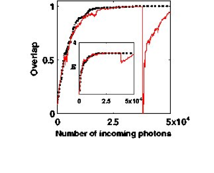
Figure 3: (Color online). Numerical simulations of the evolution in the presence of feedback of the overlap ($Tr[\varrho_{n}\varrho_{me}]$) between the state of the two atomic samples ($N=10$) and the maximal entangled state in a case in which the feedback scheme is successful (S, dotted line) in generating $\varrho_{me}$ and in a case in which the scheme is broken (B, solid line) by “anomalous” feedback angles (see text); inset: Evolution of the entanglement $E$ in the S case (dotted line) and in the B case (solid line). The values of the parameters used in the simulations are: $\eta=1$, $\chi=0.03$ (achievable with highly collimated beams), $\Omega=\pi/10$ and the total number of incoming photons is $n_{ph}=5\times 10^{4}$.

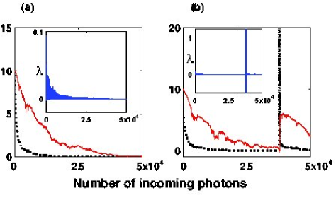
Figure 4: (Color online). (a): Numerical simulations of the evolution of $\langle\hat{J}_{x}^{+}\rangle$ (solid line) and of $\delta\hat{J}_{z}^{+}+\delta\hat{J}_{y}^{-}$ (dotted line) in the S case; inset (a): evolution of the feedback angle $\lambda$ during the S simulation; (b): Evolution of $\langle\hat{J}_{x}^{+}\rangle$ (solid line) and of $\delta\hat{J}_{z}^{+}+\delta\hat{J}_{y}^{-}$ (dotted line) in the B case. Notice that after the point in which $\langle\hat{J}_{x}^{+}\rangle<\delta\hat{J}_{z}^{+}+\delta\hat{J}_{y}^{-}$, the variances explodes. This corresponds to exploding values of $\lambda$ around that point (inset (b)). Parameter values are the same as in Fig. 3.

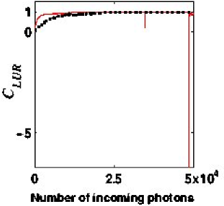
Figure 5: (Color online). Evolution of $C_{LUR}$ in a S simulation (dotted line) and in a B simulation (solid line). Positive values of $C_{LUR}$ provide a quantitative estimate of the amount of entanglement. Parameter values are the same as in Fig. 3 except that now $\eta=0.9$.

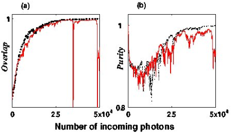
Figure 6: (Color online). (a): Evolution of the overlap in the S case (dotted line) and in the B case (solid line); (b): Evolution of the purity $Tr[\varrho_{n}^{2}]$ in the S case (dotted line) and in the B case (solid line). Notice that a successful feedback scheme has also a purification action. Obviously when the scheme is broken the purification effect is lost. Parameter values are the same as in Fig. 5.

We now discuss the different cases:

• a) No feedback: in this (PS) case the successful rate is very low: in fact, we have $\mathcal{F}\cong 6\%$ both in the ideal case ($\eta=1$) and in the more realistic case ($\eta=0.9$).

• b) Simple feedback: the action of the simple feedback relevantly increases the successful rate with respect to the pure PS. In fact, in the ideal case of perfect detection we have $\mathcal{F}\approx 54\%$: the action of the feedback on the mean value and the variances of the relevant spin operators $\hat{J}_{z}^{+}$, $\hat{J}_{y}^{-}$ and $\hat{J}_{x}^{-}$ is extremely effective, driving them to the ideal null values as the state of the two atomic clouds ($\varrho_{n}$) approaches to the maximally entangled state ($\varrho_{me}$), cf. Fig. 4(a) and 4(b). In the more realistic case ($\eta=0.9$) we obtain $\mathcal{F}\approx 24\%$. The worse result in this latter case is obviously due to the the fact that the instability of the scheme is even stressed by the mixedness of the state of the two atomic ensembles, making the action of the feedback less “precise” than the case with pure state. Moreover, the evolution of the entanglement is slower, requiring many more photons to be sent on the samples to get the same values of the overlap of the case with $\eta=1$, cf. Figs. 5 and 6. It is remarkable that, since the feedback signal depends only on the statistical moments of the spin observables, its efficiency does not depend on the exact values taken by the feedback angles. In fact, extended numerical simulations show that the feedback mechanism is not appreciably affected by perturbing the values of $\lambda$ by fluctuations of the order of $\lambda_{\pm}\times 10^{-1}\div 10^{-2}$. This is an important aspect of our scheme, which is therefore quite robust against imperfections in the actuation of the feedback operation.

• c) Modified (“adiabatic”) feedback: The only partial success of the feedback scheme is caused by the possibility that Eqs. (12) provide wrong values of the feedback angle when $\varrho_{n}\approx\varrho_{me}$. In fact, in this situation, the feedback angle $\lambda$ should uniformly go to zero, otherwise, since $\varrho_{me}$ is not invariant under the feedback rotation, the state of the two samples is transformed in a state practically orthogonal to the maximally entangled one, cf. Fig. 3. This case could happen when $\langle\hat{J}_{x}^{+}\rangle$ becomes smaller than the numerators in Eqs. (12), essentially proportional to $\delta\hat{J}_{z}^{+}+\delta\hat{J}_{y}^{-}$, cf. Fig. 4 (b). Actually, from the uncertainty relations for spin systems is easy to show that $\delta\hat{J}_{z}^{+}\delta\hat{J}_{y}^{-}\rightarrow 0$ $\Rightarrow$ $\langle\hat{J}_{x}^{+}\rangle\rightarrow 0$ BerrySanders02 ; BerrySandersNJP02 , and, due to the random jump caused by the back action of the photo-detection, in this situation it is possible to have $\langle\hat{J}_{x}^{+}\rangle<\delta\hat{J}_{z}^{+}+\delta\hat{J}_{y}^{-}$, getting in this way “exploding” values for $\lambda$, cf. inset Fig. 4 (b). However, it is possible to avoid these “anomalous” feedback angles by modifying the feedback algorithm in order to force $\lambda_{\pm}$ to go uniformly to zero as the maximally entangled state is approached. In fact, inspired by the mean values taken by $\lambda{\pm}$ in simulations in which the maximal entangled state is reached (inset Fig 4(a)), we can impose on the feedback angles of Eqs. (12) a decreasing exponential cut, a sort of adiabatic switching off, expressed as a function of the number $n$ of incoming photons: more precisely, the exponential cut is $\lambda_{cut}=x\exp(-x)$, with $x\equiv n\times 10^{-4}$, and we impose that if $|\lambda_{\pm}|\geq\lambda_{cut}$, then $\lambda=\varepsilon(\lambda_{\pm})\lambda_{cut}$, where $\varepsilon$ is the signum function; otherwise $\lambda=\lambda_{\pm}$. However, in order to not reduce the effectiveness of the feedback scheme, we switch on the correction procedure only after a high degree of entanglement is obtained, so that the state of the atomic ensembles is “close” to the maximally entangled one. The point in which the correction procedure should begin to act has to be chosen in such a way that the probability that anomalous values of $\lambda$ have already occurred is very low: by a statistical analysis of the simple feedback scheme, this point coincides roughly with $n\approx 2\times 10^{4}$. In this way we can softly, even though more slowly, drive the state of the system toward the maximally entangled state. With this procedure, the results of the numerical simulations are remarkable. In the case with $\eta=1$, we have $\mathcal{F}\approx 92\%$, and the successful rate remain remarkably high also for the realistic choice $\eta=0.9$: $\mathcal{F}\approx 78\%$. The reliability of the scheme can also be appreciated by considering stronger constrained data: in fact, if we consider overlaps greater than $0.999$, we have $90\%$ for $\eta=1$ and $64\%$ for $\eta=0.9$, while overlaps greater than $0.9999$ (practically, a full realization of the maximally entangled state) leads to $80\%$ for $\eta=1$ and $50\%$ for $\eta=0.9$.

V Conclusions

In conclusion, we have introduced an experimentally feasible, quasi-deterministic stroboscopic feedback scheme able to generate the maximally entangled state of a system composed by two mesoscopic atomic ensembles, each containing a number of atoms $N\sim 10-10^{3}$.

The feedback scheme is based on QND measurements of the total atomic population difference between the internal states of the two atomic samples, which are probed by a photon beam. Though the state of the atomic system is conditionally entangled by the photodetections, the conditional evolution does not necessarily lead to the the maximally entangled state. To this aim, we designed a scheme in which the signal obtained by the measurements, and the corresponding information on the state of the ensembles, is exploited to set up a feedback signal, formalized by an unitary operator acting on the state of the atomic samples, that drives the system into the maximal entangled state. The feedback strategy adopted is a modification of that introduced in Ref. TMW02 by Thomsen, Mancini and Wiseman.

The procedure is analyzed by numerical simulations of the conditional evolution of the state of the two atomic samples. In particular, for every simulation, we have monitored the overlap between the state of the atomic system and the maximally entangled state, and we evaluated the degree of entanglement between the two atomic ensembles. The efficiency of the protocol is quantified by the fraction of simulations in which the final value of the overlap is larger than $0.99$.

The results of the simulations show that the implementation of the feedback scheme yields a considerable enhancement of the efficiency of generating the maximal entangled state of the two atomic ensembles, compared with the case of pure probabilistic schemes without feedback. Moreover, we have shown that this efficiency can be further improved by modifying the procedure by means of an adiabatic switching off of the feedback signal.

We have shown that the scheme is able to tolerate a number of experimental imperfections, as, for instance, a limited detection efficiency. In the numerical simulations of the feedback protocol, we have considered a photocounting efficiency $\eta=0.9$: although this value is optimistic (typical laboratory photocounters are characterized by $\eta\sim 0.5$), the impressive, continuing progresses in this field give hope that very high efficiencies will be available in the near future (see for instance Ref. yama , where $\eta\simeq 0.88$ has been achieved at a particular wavelength). Nevertheless, at variance with the experimentally achieved juls01 probabilistic generation of weakly entangled states between macroscopic atomic ensembles (with typical numbers of atoms $N\sim 10^{13}$), our quasi-deterministic scheme applied to mesoscopic ensembles allows to access a presently unexplored area of entanglement production in atomic systems, even with present-day technologies against photon losses and imperfect detections.

References

- (1) K. Mølmer and A. Sørensen, Phys. Rev. Lett. 82, 1835 (1999).
- (2) C. A. Sackett, D. Kielpinski, B. E. King, C. Langer, V. Meyer, C. J. Myatt, M. Rowe, Q. A. Turchette, W. M. Itano, D. J. Wineland, and C. Monroe, Nature (London) 404, 256 (2000).
- (3) C. Cabrillo, J. I. Cirac, P. Garcia-Fernandez, and P. Zoller, Phys. Rev. A 59, 1025 (1999).
- (4) M. B. Plenio, S. F. Huelga, A. Beige, and P. L. Knight, Phys. Rev. A 59, 2468 (1999).
- (5) A. Sørensen, L. -M. Duan, J. I. Cirac, and P. Zoller, Nature (London) 409, 63 (2001).
- (6) L. -M. Duan and H. J. Kimble, Phys. Rev. Lett. 90, 253601 (2003).
- (7) J. K. Stockton, R. van Handel, and H. Mabuchi, Phys. Rev. A 70, 022106 (2004).
- (8) L. -M. Duan, J. I. Cirac, P. Zoller, and E. S. Polzik, Phys. Rev. Lett. 85, 5643 (2000).
- (9) B. Julsgaard, A. Kozhekin, and E. Polzik, Nature (London) 413, 400 (2001).
- (10) L. -M. Duan, Phys. Rev. Lett. 88, 170402 (2002).
- (11) A. Di Lisi and K. Mølmer, Phys. Rev. A. 66, 052303 (2002).
- (12) J. Sherson and K. Mølmer, Phys. Rev. A. 71, 033813 (2005).
- (13) A. Di Lisi, S. De Siena, and F. Illuminati, Phys. Rev. A 70, 012301 (2004).
- (14) L. K. Thomsen, S. Mancini, and H. M. Wiseman, Phys. Rev. A 65, 061801 (2002); L. K. Thomsen, S. Mancini, and H. M. Wiseman,, J. Phys. B 35, 4937 (2002)
- (15) J. M. Geremia J. K. Stockton, H. Mabuchi, Science, 304, 270 (2004).
- (16) D. W. Berry and B. Sanders, Phys. Rev. A 66, 012313 (2002).
- (17) D. W. Berry and B. Sanders, New J. Phys. 4, 8 (2002).
- (18) A. Peres, Quantum Theory: Concepts and Methods, Kluwer Academic Publishers (1995).
- (19) H. F. Hofmann and S. Takeuchi, Phys. Rev. A 68, 032103 (2003).
- (20) S. Takeuchi, J. Kim, Y. Yamamoto, and H. H. Hogue, Appl. Phys. Lett. 74, 1063 (1999).