Manipulation and storage of optical field and atomic ensemble quantum states

Abstract

We study how to efficiently manipulate and store quantum information between optical fields and atomic ensembles. We show how various non-dissipative transfer schemes can be used to transfer and store quantum states such as squeezed vacuum states or entangled states into the long-lived ground state spins of atomic ensembles.

I Introduction

If photons are known to be fast and robust carriers of quantum information, a major difficulty is to store their quantum state. In the continuous variable regime a number of non-classical optical field states - squeezed or entangled states - have been generated with great efficiency grangier ; lambrecht ; bowen1 ; silberhorn ; josse1 ; bowen ; glockl ; josse ; laurat . However, in order to realize scalable quantum networks bennett quantum memory elements are required to store and retrieve optical field states. To this end atomic ensembles have been widely studied as potential quantum memories lukin . Indeed, the long-lived collective spin of an atomic ensemble with two ground state sublevels appears as a good candidate for the storage and manipulation of quantum information conveyed by light zoller . Various schemes have already been studied: first, the recent ”slow-” and ”stopped-light” experiments have shown that it was possible to store a light pulse inside an atomic cloud hau ; phillips in the Electromagnetically Induced Transparency (EIT) configuration harris . EIT is known to occur when two fields are both one- and two-photon resonant with 3-level $\Lambda$-type atoms, which allows one field to propagate without dissipation through the medium. However, the storage has only been demonstrated for classical variables so far.
On the other hand, the stationary mapping of a quantum state of light (squeezed vacuum) onto an atomic ensemble, as well as the conditional entanglement of two ensembles, have been experimentally demonstrated, this time in an off-resonant Raman configuration julsgaard and in a single pass scheme. Quantum state transfers between light and atoms are also interesting in relation to ”spin squeezing” and high precision measurements wineland and have been widely studied bigelow ; kozhekin ; vernac ; molmer ; dantan1 .
In the present paper we present a model for the interaction between optical fields in cavity and atomic ensembles, and show various examples of non-destructive atom-field quantum state transfers dantan3 ; dantan4 . In the first Section we show how to write an optical field quantum state - a squeezed vacuum state - onto the ground state coherence of an atomic ensemble. We assess the efficiency of the mapping in different situations, as well as the storage into the atoms. We then consider the reverse transfer operation, from the atoms to the field, and show that it is possible to perform a quasiperfect readout of the atomic state in the field exiting the cavity. In the next Section we show how these results extend to the manipulation and storage of Einstein-Podolsky-Rosen (EPR) entangled states. In the last Section we study how to transfer the squeezing stored into one ensemble into a second.

II Quantum state transfer between field and atoms

II.1 Model system and evolution equations

The interaction considered throughout this paper is schematically represented in Fig. 1: a set of $N$ $3$-level atoms in a $\Lambda$ configuration interacts on each transition with one mode of the electromagnetic field in an optical cavity. The $3$-level system can be described using $9$ collective operators for the $N$ atoms of the ensemble: the populations $\Pi_{i}=\sum\limits_{\mu=1}^{N}\left|i\right\rangle_{\mu}\left\langle i\right|_{\mu}$ ($i=1-3)$, the components of the optical dipoles $P_{i}$ in the frames rotating at the frequency of their corresponding lasers and their hermitian conjugates and the components of the dipole associated to the ground state coherence: $P_{r}=\sum\limits_{\mu=1}^{N}\left|2\right\rangle_{\mu}\left\langle 1\right|_{\mu}$ and $P_{r}^{\dagger}$.

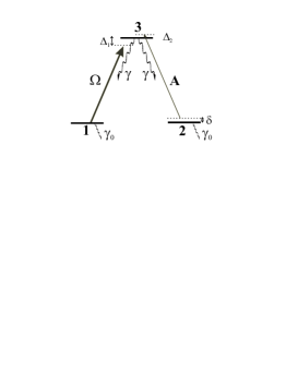
Figure 1: Three-level system in a $\Lambda$ configuration.

The atom-field coupling constants are defined by $g_{i}={\cal E}_{0i}d_{i}/\hbar$, where $d_{i}$ are the atomic dipoles, and ${\cal E}_{0i}=\sqrt{\hbar\omega_{i}/2\epsilon_{0}{\cal S}c}$ (${\cal S}$ being the beam cross-section). With this definition, the mean square value of a field is expressed in number of photons per second. To simplify, the decay constants of dipoles $P_{1}$ and $P_{2}$ are both equal to $\gamma$. In order to take into account the finite lifetime of the two ground state sublevels $1$ and $2$, we include in the model another decay rate $\gamma_{0}$, which is supposed to be much smaller than $\gamma$. We also consider that the sublevels $1$ and $2$ are repopulated with in-terms $\Lambda_{1}$ and $\Lambda_{2}$, so that the total atomic population is kept constantly equal to $N$.

The evolution of such a system is given by a set of quantum Heisenberg-Langevin equations

$$\dot{\Pi}_{1} = i\Omega^{*}P_{1}-i\Omega P_{1}^{\dagger}+\gamma\Pi_{3}-\gamma_{0}\Pi_{1}+\Lambda_{1}+F_{11}$$

$$\dot{\Pi}_{2} = ig_{2}A^{\dagger}P_{2}-ig_{2}AP_{2}^{\dagger}+\gamma\Pi_{3}-\gamma_{0}\Pi_{2}+\Lambda_{2}+F_{22}$$

$$\dot{\Pi}_{3} = -(i\Omega^{*}P_{1}-i\Omega P_{1}^{\dagger})-(ig_{2}A^{\dagger}P_{2}-ig_{2}AP_{2}^{\dagger})$$

$$\hskip 85.35826pt-2\gamma\Pi_{3}+F_{33}$$

$$\dot{P}_{1} = -(\gamma+i\Delta_{1})P_{1}+i\Omega(\Pi_{1}-\Pi_{3})+ig_{2}AP_{r}^{\dagger}+F_{1}$$

$$\dot{P}_{2} = -(\gamma+i\Delta_{2})P_{2}+ig_{2}A(\Pi_{2}-\Pi_{3})+i\Omega P_{r}+F_{2}$$

$$\dot{P}_{r} = -(\gamma_{0}-i\delta)P_{r}+i\Omega^{*}P_{2}-ig_{2}AP_{1}^{\dagger}+f_{r}$$

$$\dot{\Omega} = -(\kappa+i\Delta_{c1})\Omega+\frac{ig_{1}^{2}}{\tau}P_{1}+\sqrt{\frac{2\kappa}{\tau}}\Omega^{in}$$

$$\dot{A} = -(\kappa+i\Delta_{c2})A+\frac{ig_{2}}{\tau}P_{2}+\sqrt{\frac{2\kappa}{\tau}}A^{in}$$

where the $g_{i}$’s are assumed real, $\Omega$ is the Rabi frequency associated to the control field, $\delta=\Delta_{1}-\Delta_{2}$ is the two-photon detuning, $\kappa$ is the intracavity field decay and $\tau$ the round trip time in the cavity, so that $T=2\kappa\tau$ represents the transmission of the cavity coupling mirror. The $F$’s are standard $\delta$-correlated Langevin operators taking into account the coupling with the other cavity modes. From the previous set of equations, it is possible to derive the steady state values and the correlation matrix for the fluctuations of the whole atom-field system (see e.g. vernac ). In the following Sections we look for the best regimes for efficient quantum state transfers between fields and atoms and derive simplified equations for the transfer processes.

II.2 Decoupled equations for the fluctuations

We consider a very simple situation in which field $\Omega$ plays the role of a control parameter and field $A$ has zero mean value. In this case all the atoms are pumped in $|2\rangle$, so that only $\langle\Pi_{2}\rangle$ is non zero in steady state. The fluctuations for $\delta P_{r}$, $\delta P_{2}$ and $\delta A$ are then decoupled from the other operators fluctuations

$$\dot{\delta P_{r}} = -(\gamma_{0}-i\delta)\delta P_{r}+i\Omega\delta P_{2}+f_{r}$$ (1)

$$\dot{\delta P_{2}} = -(\gamma+i\Delta)\delta P_{2}+i\Omega\delta P_{r}+igN\delta A+F_{2}$$ (2)

$$\delta\dot{A} = -(\kappa+i\Delta_{c})\delta A+\frac{ig}{\tau}\delta P_{2}+\sqrt{\frac{2\kappa}{\tau}}\delta A^{in},$$ (3)

which allows analytical calculations and simple physical interpretations. The atomic spin associated to the ground states is aligned along $z$ at steady state: $\langle J_{z}\rangle=\langle\Pi_{2}-\Pi_{1}\rangle/2=N/2$. The spin quantum state is then given by the coherence components, $J_{x}=(P_{r}+P_{r}^{\dagger})/2$ and $J_{y}=(P_{r}-P_{r}^{\dagger})/2i$. Their commutator, $[J_{x},J_{y}]=iJ_{z}=iN/2$, is then very similar to that of the field quadrature operators: $[X_{\varepsilon},Y_{\varepsilon}]=2i$, where $X_{\varepsilon}=Ae^{-i\varepsilon}+A^{\dagger}e^{i\varepsilon}$ and $Y_{\varepsilon}=X_{\varepsilon+\pi/2}$. The field or the atomic quantum state can be represented in a symmetrical fashion by the noise ellipsoid in the conjugate variable plane. For instance, as the field is said to be squeezed when the noise of one quadrature $X_{\varepsilon}$ is less than the shot-noise value of 1, the spin component $J_{\theta}=J_{x}\cos\theta+J_{y}\sin\theta$ in the ($x,y$)-plane is said to be spin-squeezed when its variance is less than the coherent state value $|\langle J_{z}\rangle|/2$, and the degree of spin-squeezing is given by ueda

$$\Delta J^{2}_{min}=\min_{\theta}\frac{\Delta J^{2}_{\theta}}{|\langle J_{z}\rangle|/2}<1.$$ (4)

We now explicit schemes in which quantum states (squeezed or entangled states) can be transferred between field and atoms in this representation.

II.3 Writing onto atoms

For such a system two situations are particularly interesting for non-dissipative transfer processes: one is the so-called Electromagnetically Induced Transparency configuration, in which the fields are both one- and two-photon resonant ($\Delta=\delta=0$). The other is the Raman configuration, where the one-photon detuning is much larger than the exited state linewidth ($\Delta\gg\gamma$). These two interactions are rather insensitive to spontaneous emission and, therefore, very favorable to non-destructive quantum state transfer operations. For relatively bad cavities the field and the optical coherences evolve rapidly as compared to the ground state coherence. In this limit it is possible to adiabatically eliminate these operators and derive simple analytical equations for the ground state observables:

$$\delta\dot{J}_{x} = -\gamma_{\varepsilon}\delta J_{x}-\beta_{\varepsilon}\delta X_{\varepsilon}^{in}+\tilde{f}_{x}$$ (5)

$$\delta\dot{J}_{y} = -\gamma_{\varepsilon}\delta J_{y}-\beta_{\varepsilon}\delta Y_{\varepsilon}^{in}+\tilde{f}_{y}$$ (6)

where $\varepsilon$ stands for the situation considered: ”EIT” ($\Delta=0$) is denoted by $\varepsilon=0$, whereas the ”Raman” configuration ($\Delta\gg\gamma$) corresponds to $\varepsilon=\pi/2$. With these notations $\gamma_{\varepsilon}=\gamma_{0}+\Gamma_{\varepsilon}$ is the effective pumping rate for the fluctuations [$\Gamma_{0}=\Gamma_{E}/(1+2C)$ in EIT and $\Gamma_{\pi/2}=(1+2C)\Gamma_{R}$ in a Raman configuration]. $\beta_{\varepsilon}$ is the coupling coefficient between the incident field and the atomic coherence [$\beta_{0}=gN\Omega/\gamma(1+2C)\sqrt{T}$ and $\beta_{\pi/2}=gN\Omega/\Delta\sqrt{T}$], and the $\tilde{f}$’s are effective quantum Langevin operators accounting for dissipation. In both cases the effective two-photon detuning and the effective cavity detuning are set to 0. Both situations derive from formally similar effective Hamiltonians

$$H_{\varepsilon}=\hbar\frac{2\beta_{\varepsilon}}{N}\left[J_{x}Y_{\varepsilon}^{in}-J_{y}X_{\varepsilon}^{in}\right].$$ (7)

Since this Hamiltonian is nothing but the coupling between two harmonic oscillators, the physical interpretation is clear: if one knows the input field state $A^{in}$ variance matrix one can deduce that of the atomic spin. In EIT, for instance, and for a broadband squeezed vacuum input, the spin-squeezed component angle $\theta_{sq}$ will be that of the field squeezed quadrature: $\theta_{sq}=\varepsilon_{sq}$. In a Raman configuration a $\pi/2$ rotation of the spin should be performed: $\theta_{sq}=\varepsilon_{sq}+\pi/2$. In both cases the minimum variance takes a similar form

$$\Delta J^{2}_{min}=\frac{2C}{1+2C}\frac{\Gamma_{\varepsilon}}{\gamma_{\varepsilon}}e^{-2r}+\frac{\gamma_{0}}{\gamma_{\varepsilon}}+\frac{1}{1+2C}\frac{\Gamma_{\varepsilon}}{\gamma_{\varepsilon}}$$ (8)

where $e^{-2r}$ is the incident field squeezing. The first term ($\varpropto e^{-2r}$) reflects the incident field state, the second ($\varpropto\gamma_{0}$) is the noise contribution associated to the loss of ground state coherence and the third ($\varpropto\Gamma_{\varepsilon}$) is the noise contribution coming from spontaneous emission.

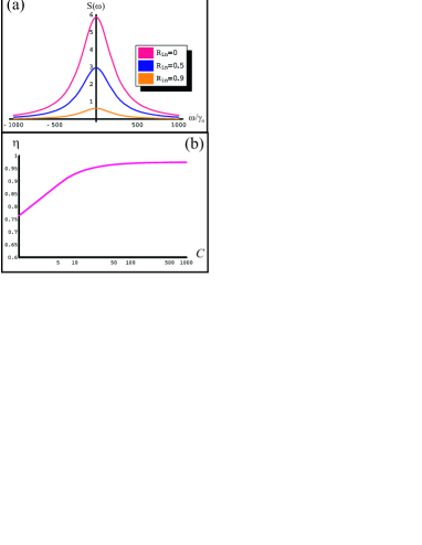
Figure 2: (a) Atomic noise spectra for the least noisy spin component, for different values of the input squeezing $R_{in}=1-e^{-2r}$. The effective pumping rate and the cooperativity are the same for each curve ($C=100,\gamma_{\varepsilon}=0.075\gamma$). (b) Optimized transfer efficiency versus cooperativity.

Consequently, one sees that a good quantum state transfer - $\Delta J^{2}_{min}\sim e^{-2r}$ - occurs in the regime $C\gg 1$ and $\gamma_{0}\ll\Gamma_{\varepsilon}\ll\gamma,\kappa$. A useful quantity to characterize the quality of the quantum state transfer is provided by the transfer efficiency $\eta=(1-\Delta J^{2}_{min})/(1-e^{-2r})$, which can be written as

$$\eta_{\varepsilon}=\frac{2C}{1+2C}\frac{\Gamma_{\varepsilon}}{\gamma_{0}+\Gamma_{\varepsilon}}$$ (9)

In Fig. 2(b) we show the transfer efficiency versus the cooperativity. For each value of $C$ the optical pumping was optimized numerically in order to maximize the efficiency dantan3 . A high efficiency is possible for rather small values of the cooperativity.

Note that, in this case, one could also define a standard quantum limit for the atomic noise by looking at the atomic noise spectrum. In this low-frequency approximation the atomic coherence noise spectra have a Lorentzian shape with FHWM given by $2\gamma_{\varepsilon}$. For the squeezed component this Lorentzian has a peak value decreased by a factor $e^{-2r}$ as compared to that of the corresponding coherent state [see Fig. 2(a)]. However, this notion of standard quantum limit at a given frequency is only relevant when comparing with the noise spectrum of a coherent spin state under the same conditions (same pumping strength $\gamma_{\varepsilon}$, same number of atoms…). Besides, $\gamma_{\varepsilon}$ represents the quantum memory storage frequency bandwidth. An interesting feature of this cavity scheme is that it is much broader than the natural linewidth $\gamma_{0}$.

This simplified model can be shown to be in excellent agreement with full quantum calculations in the regime considered. A more detailed study of what happens when $\Gamma_{\varepsilon}$ is increased, when the detunings are non-zero or when arbitrary field states for $A$ are used can be found in Ref. dantan3 .

II.4 Storage and readout

The squeezing transfer can be considered completed after a time of a few $1/\gamma_{\varepsilon}$. If all fields are abruptly switched off one is left with a spin squeezed atomic ensemble. The atomic squeezing decays very slowly on a timescale given by $1/\gamma_{0}$. After a storage time $t_{s}$, small with respect to this decay time, one can retrieve the atomic state into the field exiting the cavity by switching on again only the control field. Indeed, neglecting $\gamma_{0}$ and in the regime $\Gamma_{\varepsilon}\ll\gamma,\kappa$ the outgoing field mode can be shown to be

$$\delta X_{\varepsilon}^{out}(t) = \delta X_{\varepsilon}^{in}(t)-\alpha\delta J_{\varepsilon}(0)e^{-\Gamma_{\varepsilon}t}$$

$$-2\eta^{2}[\delta X_{\varepsilon}^{in}(t)-\Gamma_{\varepsilon}\int_{0}^{t}e^{-\Gamma_{\varepsilon}(t-s)}\delta X_{\varepsilon}^{in}(s)ds]$$

$$+\beta[\delta X_{v\varepsilon}(t)-\Gamma_{\varepsilon}\int_{0}^{t}e^{-\Gamma_{\varepsilon}(t-s)}\delta X_{v\varepsilon}(s)ds],$$

with $\alpha=\eta\sqrt{8\Gamma_{\varepsilon}/N}$, $\beta=2\eta/\sqrt{1+2C}$ and $X_{v\varepsilon}$ is a white noise operator corresponding to a normalized Langevin operator with unity spectrum. $\eta=2C/(1+2C)$ is the efficiency for $\gamma_{0}=0$, independent of the interaction considered. The terms in $X_{\varepsilon}^{in}$, $X_{v\varepsilon}$ are intrinsic and added field noise terms, whereas the term in $J_{\varepsilon}$ provides the quantum information relative to the incident atomic state. The two-time correlation function has a much simpler form

$$\mathcal{C}(t,t^{\prime}) \equiv \langle\delta X_{\varepsilon}^{out}(t)\delta X_{\varepsilon}^{out}(t^{\prime})\rangle$$

$$= \delta(t-t^{\prime})-\frac{2C}{1+2C}2\Gamma_{\varepsilon}\left[1-\Delta^{2}J_{\varepsilon}(0)\right]e^{-\Gamma_{\varepsilon}(t+t^{\prime})}$$

In the absence of coupling [$\Gamma_{\varepsilon}=0$], or for a coherent spin state [$\Delta J_{\varepsilon}^{2}=1$], one naturally retrieves a shot-noise limited free field, with a $\delta$-correlation function. However, if the atoms are spin-squeezed one transitorily observes sub-shot noise fluctuations for the outgoing field. It was shown in dantan3 that it is possible to measure the atomic state with almost $100\%$ efficiency using a homodyne detection and correctly choosing the local oscillator temporal profile - or, equivalently, by choosing the right electronic gain in the detection process. Using an optimal matching in $e^{-\Gamma_{\varepsilon}t}$, adapted to the atomic temporal response, the readout efficiency, defined as the ratio of field squeezing to atomic squeezing (at switching time), is then also given by $\eta$. Taking into account that the atomic squeezing has decreased by a factor $e^{-2\gamma_{0}t_{s}}$ during storage, the global efficiency of the quantum memory is then $\eta^{2}e^{-2\gamma_{0}t_{s}}$.

III EPR-correlated atomic ensembles

Figure 3: Scheme for entanglement storage into two ensembles.

In this Section we show how to generalize the previous quantum state transfer to quantum correlated states, or EPR states, which are of great importance in many quantum information protocols in the continuous variable regime. As mentioned earlier such states are now readily produced by different sources and with very good efficiency bowen ; glockl ; josse ; laurat . We therefore assume that we dispose of a pair of EPR-entangled vacuum fields, $A_{1}$ and $A_{2}$, and of a pair of identical ensembles (1) and (2), as shown in Fig. 3. The amount of EPR-type correlations between the incident field modes is quantified using the inseparability criterion duan

$$\mathcal{I}_{f}^{in}=\frac{1}{2}[\Delta^{2}(X_{1}^{in}-X_{2}^{in})+\Delta^{2}(Y_{1}^{in}+Y_{2}^{in})]<2$$ (12)

For the spins $J_{x1}-J_{x2}$ and $J_{y1}+J_{y2}$ are the equivalent of the EPR operators, since $\langle[J_{x1}-J_{x2},J_{y1}+J_{y2}]\rangle=i\langle J_{z1}-J_{z2}\rangle=0$ when spins 1 and 2 are equal and parallel. A similar criterion to (12) can be derived for the inseparability of spins 1 and 2

$$\Delta^{2}(J_{x1}-J_{x2})+\Delta^{2}(J_{y1}+J_{y2})<|\langle J_{z1}\rangle|+|\langle J_{z2}\rangle|=N$$

As in the previous Section ”EIT”- or ”Raman”-type interactions with both ensembles lead to coupling between the incident EPR-fields and the spin coherence components

$$\frac{d}{dt}(\delta J_{x1}-\delta J_{x2}) = -\gamma_{\varepsilon}(\delta J_{x1}-\delta J_{x2})$$

$$-\beta_{\varepsilon}(\delta X_{1\varepsilon}^{in}-\delta X_{2\varepsilon}^{in})+\tilde{f}_{x1}-\tilde{f}_{x2}$$

$$\frac{d}{dt}(\delta J_{y1}+\delta J_{y2}) = -\gamma_{\varepsilon}(\delta J_{y1}+\delta J_{y2})$$

$$-\beta_{\varepsilon}(\delta Y_{1\varepsilon}^{in}+\delta Y_{2\varepsilon}^{in})+\tilde{f}_{y1}+\tilde{f}_{y2}$$

and one can show that the field entanglement is efficiently transferred to the spins dantan4

$$\mathcal{I}_{at}=\frac{2C}{1+2C}\frac{\Gamma_{\varepsilon}}{\gamma_{\varepsilon}}\;\mathcal{I}_{f}+2\left[\frac{\gamma_{0}}{\gamma_{\varepsilon}}+\frac{\Gamma_{\varepsilon}}{(1+2C)\gamma_{\varepsilon}}\right]$$ (15)

where $\mathcal{I}_{at}=\frac{2}{N}[\Delta^{2}(J_{x1}-J_{x2})+\Delta^{2}(J_{y1}+J_{y2})]$ stands for the atomic entanglement (normalized to 2). The same conclusions hold: for a good cooperative behavior ($C\gg 1$) and for $\gamma_{0}\ll\gamma_{\varepsilon}\ll\gamma,\kappa$, the added noise terms ($\varpropto 1/(1+2C)$ and $\gamma_{0}$) are negligible compared to the coupling, and the atomic entanglement is close to the initial field entanglement, $\mathcal{I}_{at}\sim\mathcal{I}_{f}$.
The same readout scheme as previously can be applied to retrieve entanglement in a transient manner between the outgoing fields. This entanglement can be measured using the techniques developed in Refs. josse ; dantan3 ; josse2 . Note that the lifetime of this entanglement is given by the phenomenological time constant $1/\gamma_{0}$ introduced in our model. For cold atoms it can represent the loss of atoms out of the trap, and for atomic vapors the depolarizing time. We have neglected the collisions leading to a depolarization of the spin, which is legitimate for cold atoms, but should be considered for vapors if one were to evaluate precisely the storage time of the quantum memory.

IV Pseudo-quantum repeater

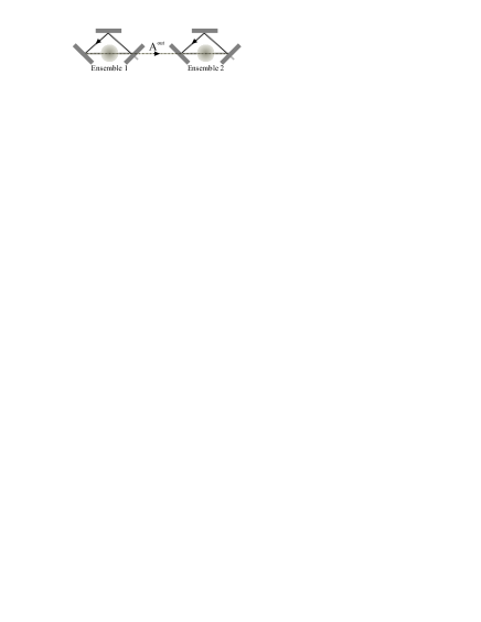
Figure 4: Scheme for the ”pseudo” quantum repeater.

We assume that we dispose of two identical atomic ensembles [Fig. 4] and that, using the techniques of Sec. II.3, we have spin-squeezed ensemble 1 to some degree $e^{-2r_{1}}$ on the $x$-component and that it is in a minimum uncertainty state ($\Delta J_{y1}^{2}=e^{2r_{1}}$). Spin 2 is initially in a coherent spin state aligned along $z$. If we perform an optical readout of ensemble 1 by switching on the control field in the first cavity the outgoing field is squeezed, as can be seen from (II.4). It can then be used as input for the spin in the second cavity

$$\delta\dot{J}_{x2} = -\gamma_{\varepsilon}\delta J_{x2}-\beta_{\varepsilon}\delta X_{\varepsilon}^{out}+\tilde{f}_{x2}$$ (16)

$$\delta\dot{J}_{y2} = -\gamma_{\varepsilon}\delta J_{y2}-\beta_{\varepsilon}\delta Y_{\varepsilon}^{out}+\tilde{f}_{y2}$$ (17)

where $X^{out}_{\varepsilon}$ and $Y^{out}_{\varepsilon}$ are input fields out of the first cavity, the expression of which is given by (II.4). In the previous equations we have neglected the transit time from one cavity to the other. The variances of spin 2 coherence components can be calculated from Eqs. (II.4), (16) and (17); one gets, after normalization by the atomic shot-noise $N/4$,

$$\Delta J_{x2}^{2}(t) = 1-\eta^{4}(2\gamma_{\varepsilon}t)^{2}e^{-2\gamma_{\varepsilon}t}[1-e^{-2r_{1}}]$$ (18)

$$\Delta J_{y2}^{2}(t) = 1+\eta^{4}(2\gamma_{\varepsilon}t)^{2}e^{-2\gamma_{\varepsilon}t}[e^{2r_{1}}-1]$$ (19)

The squeezing in the second cavity is maximum for $t=1/\gamma_{\varepsilon}$ and is related to the squeezing in the first cavity:

$$1-e^{-2r_{2}}=\frac{4}{e^{2}}\eta^{4}[1-e^{-2r_{1}}]$$ (20)

Since $4/e^{2}\simeq 0.54$, only a little bit more than half of the initial squeezing can be transferred to the second ensemble with direct method.

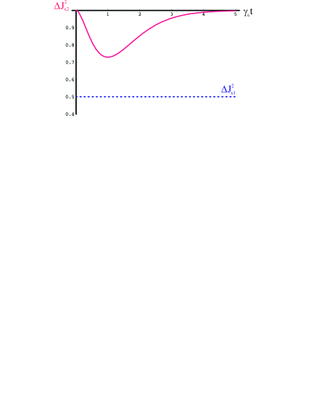
Figure 5: Minimal variance of spin 2 as a function of time: the squeezing increases to a maximum for $\gamma_{\varepsilon}t\simeq 1$ and then decreases back to 0. The initial squeezing in ensemble 1 is $1-e^{-2r_{1}}=0.5$.

Another way to understand this imperfect transfer is to go to the Fourier domain and see that the first ensemble response has a spectral width given by $\gamma_{\varepsilon}$, and the input squeezing spectrum of $X^{out}$ is itself multiplied by the same response function for spin 2. The atomic noise spectrum in the second cavity is then the product of two Lorentzian profiles with equal width $\gamma_{\varepsilon}$. The atomic noise is then at best the integral of this squared Lorentzian, which results in this approximately 50% quantum state transfer. Note that having different widths for the readout of spin 1 and the writing on spin 2 does not improve the result. To fully transfer the state of spin 1 to spin 2 one actually needs a more refined protocol, atomic teleportation kuzmich ; dantan5 , which requires entanglement of the kind used in Sec. III.

V Conclusion

We have presented a quantum model in which non-dissipative interactions provide quasiperfect quantum state transfer between optical fields and atomic ensembles spins. Field squeezed states and EPR-entangled states can be stored with high efficiency into atoms for a long time, and read out at will in the fields exiting the cavities. Since both the squeezing and the entanglement are conserved in such operations these results should be of importance for the realization of robust quantum information and communication networks involving optical fields and atomic ensembles. Last, we examined the possibility to transfer by these techniques the squeezing of a first atomic ensemble to a second. However, the efficiency of the second mapping is limited to about 50%. To achieve a perfect mapping one needs to perform a full quantum teleportation protocol. This can be done by combining all the ingredients presented in this paper dantan5 .

References

- (1) Grangier P., Slusher R.E., Yurke B. and LaPorta A., Phys. Rev. Lett. 59, 2153 (1987).
- (2) Lambrecht A., Coudreau T., Steimberg A.M. and Giacobino E., Europhys. Lett. 36, 93 (1996).
- (3) Bowen W.P., Schnabel R., Bachor H.A. and Lam P.K., Phys. Rev. Lett. 88, 093601 (2002).
- (4) Silberhorn C., Lam P.K., WeißO., König F., Korolkova N. and Leuchs G., Phys. Rev. Lett. 86, 4267 (2001).
- (5) Josse V., Dantan A., Vernac L., Bramati A., Pinard M. and Giacobino E., Phys. Rev. Lett. 91, 103601 (2003).
- (6) Bowen W.P., Treps N., Schnabel R. and Lam P.K., Phys. Rev. Lett. 89, 253601 (2002).
- (7) Glöckl O., Lorenz S., Marquardt C., Heersink J., Brownnutt M., Silberhorn C., Pan Q., van Loock P., Korolkova N. and Leuchs G., Phys. Rev. A 68, 012319 (2003);
- (8) Josse V., Dantan A., Bramati A., Pinard M. and Giacobino E., Phys. Rev. Lett. 92, 123601 (2004).
- (9) Laurat J., Coudreau T., Keller G., Treps N. and Fabre C., (2004), quant-ph/0403224.
- (10) DiVincenzo D.P., Science, 270, 255 (1995); Furusawa A., Sorensen J., Braustein S. Fuchs C., Kimble H.J. and Polzik E.S., Science, 282, 706 (1998); Braustein S.L. and Kimble H.J., Phys. Rev. A 61, 042302 (2000).
- (11) Lukin M.D., Rev. Mod. Phys. 75, 457 (2003); Duan L.M., Cirac J.I., Zoller P. and Polzik E.S., Phys. Rev. Lett. 85, 5643 (2000).
- (12) Duan L.M., Lukin M.D., Cirac J.I. and Zoller P., Nature (London) 414, 413 (2001).
- (13) Harris S.E. and Hau L.V., Phys. Rev. Lett. 82, 4611 (1999); Liu C., Dutton Z., Behroozi C.H., and Hau L.V., Nature (London) 409, 490 (2001).
- (14) Phillips D.F., Fleischhauer A., Mair A., and Walsworth R.L., and Lukin M.D., Phys. Rev. Lett. 86, 783 (2001).
- (15) Harris S.E., Phys. Today 50, 36 (1997).
- (16) Hald J., Sørensen J.L., Schori C., and Polzik E.S., Phys. Rev. Lett. 83, 1319 (1999); Julsgaard B., Kozhekin A. and Polzik E.S., Nature 413, 400 (2001).
- (17) Wineland D.J., Bollinger J.J., Itano W.M., and Heinzen D.J., Phys. Rev. A 50, 67 (1994).
- (18) Kuzmich A., Mandel L., and Bigelow N.P., Phys. Rev. Lett. 85, 1594 (2000);
- (19) Kozhekin A.E., Mølmer K., and Polzik E.S., Phys. Rev. A 62, 033809 (2000).
- (20) Vernac L., Pinard M. and Giacobino E., Phys. Rev. A 62, 063812 (2000).
- (21) Poulsen U.V. and Mølmer K., Phys. Rev. Lett. 87, 123601 (2001).
- (22) Dantan A., Pinard M., Josse V., Nayak S., and Berman P.R., Phys. Rev. A 67, 045801 (2003).
- (23) Dantan A. and Pinard M., Phys. Rev. A 69, 043810 (2004).
- (24) Dantan A., Bramati A., and Pinard M., Europhys. Lett. to be published (2004), quant-ph/0405020.
- (25) Kitagawa M. and Ueda M., Phys. Rev. A 47, 5138 (1993).
- (26) Duan L.M., Giedke G., Cirac. J.I., and Zoller P., Phys. Rev. Lett. 84, 2722 (2000); Simon R., Phys. Rev. Lett. 84, 2726 (2000).
- (27) Josse V., Dantan A., Bramati A., and Giacobino E., J. Opt. B: Quant. Semiclass. 6, S532 (2004).
- (28) Kuzmich A. and Polzik E.S., Phys. Rev. Lett. 85, 9007 (2000).
- (29) Dantan A., Treps N., Bramati A., and Pinard M., in preparation.