Quantum noise and mixedness of a pumped dissipative non-linear oscillator

Abstract

Evolutions of quantum noise, characterized by quadrature squeezing parameter and Fano factor, and of mixedness, quantified by quantum von Neumann and linear entropies, of a pumped dissipative non-linear oscillator are studied. The model can describe a signal mode interacting with a thermal reservoir in a parametrically pumped cavity with a Kerr non-linearity. It is discussed that the initial pure states, including coherent states, Fock states, and finite superpositions of coherent states evolve into the same steady mixed state as verified by the quantum relative entropy and the Bures metric. It is shown analytically and verified numerically that the steady state can be well approximated by a nonclassical Gaussian state exhibiting quadrature squeezing and sub-Poissonian statistics for the cold thermal reservoir. A rapid increase is found in the mixedness, especially for the initial Fock states and superpositions of coherent states, during a very short time interval, and then for longer evolution times a decrease in the mixedness to the same, for all the initial states, and relatively low value of the nonclassical Gaussian state.

Keywords: quantum entropy, quadrature squeezing, sub-Poissonian statistics, Wigner function, Husimi functions, Kerr non-linearity, Schrödinger cats, steady states.

I Introduction

Quantum noise and mixedness are properties central for quantum theory neumann . It is obvious that a pure signal state interacting with a thermal environment loses its purity and turns into a mixed state. Since real optical devices suffer from losses, it is important to study their influence on the noise and mixedness during the state evolution.

In the case of interactions of a small number of the signal and reservoir modes, the noise and mixedness parameters periodically rise and fall. But in the case of the signal interacting with an infinite number of the reservoir modes, the evolution is irreversible and after a few characteristic time intervals, the signal mode transforms into an asymptotic steady state depending on external parameters of the system, e.g., an external classical pump. One can show that when the pump is turned off, final steady state of the signal will be the pure vacuum state, but when the pump is turned on, the steady state is not the vacuum but a mixed nonclassical state. We show further that the steady state can be properly approximated by a nonclassical Gaussian state (NCGS).

In the next sections we will investigate a particular example of a non-linear interaction, i.e., a nontrivial dynamics of initial signal modes in a pumped resonator with a non-linear Kerr medium when losses are included (see, e.g., drummond1 ; drummond2 ; kheru ). We are interested mainly in the quantum noise and mixedness (purity) evolutions of the signal mode. We discuss three different types of the signal initial states including coherent states, Fock states and superpositions of coherent states. We study the influence of the losses, pump and non-linearity on the signal evolution, in particular the fast decoherence of the initial coherent superpositions.

II Interaction model

A pumped non-linear oscillator can be described in the interaction picture by the following Hamiltonian drummond1 ; drummond2 :

$$\hat{H} = \hat{H}_{I}+\hat{H}_{R},$$ (1)

$$\hat{H}_{I} = \mathrm{i}(p\hat{a}^{{\dagger}}-p^{\ast}\hat{a})+G\hat{a}^{{\dagger}2}\hat{a}^{2}.$$ (2)

where $\hat{a}$ and $\hat{a}^{{\dagger}}$ are the annihilation and creation operators of the signal mode, respectively. The first term in Hamiltonian $\hat{H}_{I}$ describes a pump process with the complex amplitude $p$, the second term represents a Kerr process with the non-linear interaction constant $G$ and $\hat{H}_{R}$ is the term describing the interaction of the signal mode with the cold thermal reservoir. For simplicity we use the units where $\hbar=1$. The model can be used in a description of, e.g., a parametrically pumped cavity with a Kerr non-linearity. We adopt the Heisenberg-Langevin approach perina , in which the Heisenberg equation for the signal mode reads is

$$\frac{\mathrm{d}\hat{a}}{\mathrm{d}t}=p-2\mathrm{i}G\hat{a}^{{\dagger}}\hat{a}^{2}-\gamma_{0}\hat{a}+\hat{\cal L},$$ (3)

where $\hat{\cal L}$ is the Langevin force and $\gamma_{0}$ is the loss parameter. For the optical modes at room temperature, the number of thermal photons can be assumed negligible. Therefore, in the following we assume the zero-temperature approximation. In that case the standard rules hold for the Langevin force:

$$\langle\hat{\cal L}(t_{1})\hat{\cal L}(t_{2})\rangle = \langle\hat{\cal L}^{{\dagger}}(t_{1})\hat{\cal L}(t_{2})\rangle=\langle\hat{\cal L}(t_{1})\rangle=0,$$

$$\langle\hat{\cal L}(t_{1})\hat{\cal L}^{{\dagger}}(t_{2})\rangle = 2\gamma_{0}\delta(t_{1}-t_{2}).$$ (4)

For the linear interaction ($G=0$) of the signal mode, an analytical solution can be found. For the coherent initial state $|\alpha\rangle$, the solution is $|\psi\rangle=|\alpha\left(t\right)\rangle$ with the time-dependent complex amplitude

$$\alpha\left(t\right)=\alpha\mathrm{e}^{-\gamma_{0}t}+\frac{p}{\gamma_{0}}\left(1-\mathrm{e}^{-\gamma_{0}t}\right).$$ (5)

So the initial coherent state with the amplitude $\alpha$ finally evolves into another coherent state with the amplitude $p/\gamma_{0}$. The evolution is essentially finished during a short period equal to the first few characteristic times $\tau=1/\gamma_{0}$. For the model without a pump, the initial state turns into the vacuum state.

In the non-linear Kerr interaction case, the evolution cannot be solved analytically for arbitrary evolution times and suitable numerical methods have to be used. The state evolution in this case is much more complex and is the main subject of our study. Under reasonable assumptions some analytical approximations can be derived as well. After presenting our precise numerical results, we will also give an exact quantum steady-state solution and its semiclassical approximation in the long-time limit.

Alternatively we can start from the Liouville equation, which leads to the following master equation

$$\frac{\mathrm{d}\hat{\rho}}{\mathrm{d}t}=\frac{1}{\mathrm{i}\hbar}[\hat{H},\hat{\rho}]=\frac{1}{\mathrm{i}\hbar}[\hat{H}_{I},\hat{\rho}]+\hat{R},$$ (6)

where $\hat{R}$ for the zero temperature reservoir stands for

$$\hat{R}=\frac{1}{i\hbar}[\hat{H}_{R},\hat{\rho}]=\gamma_{0}\left(2\hat{a}\hat{\rho}\hat{a}^{{\dagger}}-\hat{a}^{{\dagger}}\hat{a}\hat{\rho}-\hat{\rho}\hat{a}^{{\dagger}}\hat{a}\right).$$ (7)

Master equation (6) can simply be expressed in the Fock basis with the density matrix in the form

$$\hat{\rho}=\sum_{nm}\rho_{mn}|m\rangle\langle n|$$ (8)

leading to a set of ordinary linear differential equations for the density matrix elements $\rho_{mn}=\langle m|\hat{\rho}|n\rangle$. For weak interaction fields the differential equations can be solved numerically. The exact quantum results presented in this article are obtained by applying this method.

To visualize evolution of quantum states (pure or mixed) generated in our system, we apply the Husimi and Wigner functions, which are the special cases of the Cahill-Glauber $s$-parametrized quasidistribution function ${\cal W}^{(s)}(\beta)$ defined for $-1\leq s\leq 1$ as follows cahill :

$${\cal W}^{(s)}(\beta) = \frac{1}{\pi}\,{\rm Tr}\,\{\hat{\rho}\,\hat{T}^{(s)}(\beta)\},$$ (9)

where $\hat{\rho}$ is the density matrix of the field and

$$\hat{T}^{(s)}(\beta) = \frac{1}{\pi}\int\exp(\beta\xi^{*}-\beta^{*}\xi)\hat{D}^{(s)}(\xi)\,{\rm d}^{2}\xi,$$ (10)

and $\hat{D}^{(s)}(\xi)={\rm e}^{s|\xi|^{2}/2}\hat{D}(\xi)$ with $\hat{D}(\xi)$ being the displacement operator. The quasidistribution ${\cal W}^{(s)}(\beta)$ in the number-state basis can be calculated as cahill :

$${\cal W}^{(s)}(\beta) = \frac{1}{\pi}\sum_{m,n}\rho_{mn}\langle n|\hat{T}^{(s)}(\beta)|m\rangle,$$ (11)

where

$$\langle n|\hat{T}^{(s)}(\beta)|m\rangle=\left(\frac{n!}{m!}\right)^{1/2}\left(\frac{2}{1-s}\right)^{m-n+1}\left(\frac{s+1}{s-1}\right)^{n}$$

$$\hskip 11.38109pt\times\;(\beta^{*})^{m-n}\exp\left(-\frac{2|\beta|^{2}}{1-s}\right)L_{n}^{m-n}\left(\frac{4|\beta|^{2}}{1-s^{2}}\right)$$

(12)

given in terms of the associate Laguerre polynomials $L_{n}^{m-n}(x)$. Eq. (12) for $s\rightarrow-1$ goes into the simple expression

$$\langle n|\hat{T}^{(-1)}(\beta)|m\rangle = \exp\left(-|\beta|^{2}\right)\frac{\beta^{n}(\beta^{*})^{m}}{\sqrt{n!m!}}$$ (13)

as can be derived by observing that $\lim_{\epsilon\rightarrow 0}\epsilon^{n}L_{n}^{m-n}(\frac{y}{\epsilon})=(-y)^{n}/n!$. Eq. (12) can also be applied for $s\rightarrow 1$ if the limit is taken carefully (see e.g. tanas ). The special cases of ${\cal W}^{(s)}(\beta)$ for $s=-1,0,1$ are known as the Husimi $Q$-function, the Wigner $W$-function and Glauber-Sudarshan $P$-function, respectively. For example, the $s$-parametrized quasidistribution function for coherent state $|\alpha\rangle$ is given by the Gaussian distribution ${\cal W}^{(s)}(\beta)=2/[\pi(1-s)]\exp[-2|\beta-\alpha|^{2}/(1-s)]$, which for $s=1$ becomes Dirac’s delta $\delta(\beta-\alpha)$. If a given state is described by the $P$-function, which is positive definite and no more irregular than Dirac’s delta, then the state is classical, otherwise the state is considered to be nonclassical. We use this criterion to show that the steady state of our system is nonclassical.

III Measures of quantum noise and mixedness

Quantum noise properties of nonclassical light can be analysed in terms of the Fano factor and quadrature noise variances. The first parameter corresponds to direct photo-pulse detections, while the second is related to homodyne detection schemes. The Fano factor is defined by

$$F=\frac{\langle n^{2}\rangle-\langle n\rangle^{2}}{\langle n\rangle}.$$ (14)

which for Poissonian states satisfies $F=1$, while for sub- and super-Poissonian states is $F<1$ and $F>1$, respectively. In particular, the Fock states are sub-Poissonian with $F=0$ independently of the number of photons, coherent states are Poissonian ($F=1$), while thermal chaotic states are super-Poissonian since $F=1+2\langle n\rangle>1$. The quadrature noise squeezing parameter $S$ is defined as the minimum variance $S=\min_{\theta}\langle(\Delta X_{\theta})^{2}\rangle$ over all possible values of phase $\theta\in\left(0,2\pi\right)$ of the general quadrature operator $X_{\theta}=\hat{a}\mathrm{e}^{-\mathrm{i}\theta}+\hat{a}^{{\dagger}}\mathrm{e}^{\mathrm{i}\theta}$. For a coherent state $S=1$, while a state with $S<1$ is referred to as the quadrature squeezed light, since it has lower noise level than the coherent or vacuum state.

The most natural measure of mixedness of a state, given by $\hat{\rho}$, is the von Neumann entropy neumann

$$E=-\langle\ln\hat{\rho}\rangle=-\mathrm{Tr}\{\hat{\rho}\ln\hat{\rho}\}.$$ (15)

Density matrix $\hat{\rho}$ of any mixed state can be expressed as the incoherent sum

$$\hat{\rho}=\sum_{k=1}^{N}p_{k}|\psi_{k}\rangle\langle\psi_{k}|,$$ (16)

of the orthogonal pure states $|\psi_{k}\rangle$, where $p_{k}$ are their weight factors being eigenvalues of the density matrix $\hat{\rho}$. As follows from the general properties of the density matrix, it holds $0\leq p_{k}\leq 1$ and $\sum_{k=1}^{N}p_{k}=1$. Thus, the von Neumann entropy can be expressed as

$$E=-\sum_{k=1}^{N}p_{k}\ln p_{k}\geq 0.$$ (17)

Another useful measure of mixedness is the linear entropy $L$ defined as

$$L=1-\mathrm{Tr}\{\hat{\rho}^{2}\},$$ (18)

where the second term in (18) is referred to as the purity $P$ of the state

$$P=\mathrm{Tr}\{\hat{\rho}^{2}\}=\sum_{k=1}^{N}p_{k}^{2}.$$ (19)

The mixedness $L$ and the purity $P$ are complementary in the sense that whenever the entropy increases the purity falls. For completeness, we note other generalized measures of the mixedness including (see, e.g., zyczkowski ): the Renyi entropies defined by $H_{q}=(\ln\mathrm{Tr}\{\rho^{q}\})/\left(1-q\right)$ ($q=2,3,...$), the Neumann-Renyi entropy given by $H_{2}=-\ln\mathrm{Tr}\{\hat{\rho}^{2}\}=-\ln P$ or the participation ratio defined to be $R=1/\mathrm{Tr}\{\rho^{2}\}=1/P$.

It is easy to show the following properties of the mixedness parameters $E$ and $L$: For any pure state it holds $E=L=0$. For a mixture of two orthogonal states it holds $0\leq L\leq 1/2$ and $0\leq E\leq\ln 2$. For a balanced mixture of two orthogonal modes $p_{1}=p_{2}=1/2$ it holds $L=1/2$ and $E=\ln 2$ as their maxima. For a mixed state composed of $N$ orthogonal pure states it holds $0\leq L\leq(N-1)/N$ and $0\leq E\leq\ln N$. For a homogeneous superposition it is $p_{k}=1/N$ and therefore $L=(N-1)/N$ and $E=\ln N$. So, for a state strongly mixed with the reservoir, $L$ can increase to one and $E$ to infinity.

For thermal or chaotic states, the density matrix is diagonal with

$$\rho_{kk}=p_{k}=\frac{\langle n\rangle^{k}}{\left(1+\langle n\rangle\right)^{1+k}},$$ (20)

implying that the linear entropy is

$$L_{\mathrm{chaot}}=\frac{2\langle n\rangle}{1+2\langle n\rangle}$$ (21)

and the corresponding von Neumann entropy is

$$E_{\mathrm{chaot}}=-\ln\frac{\langle n\rangle^{\langle n\rangle}}{\left(1+\langle n\rangle\right)^{1+\langle n\rangle}}.$$ (22)

Here, $\langle n\rangle$ stands for the number of photons in the chaotic mode. For the vacuum state $\langle n\rangle=0$, which is a pure state, we get $E=L=0$, while for the chaotic state with $\langle n\rangle=1$ we get $E=\allowbreak\ln 4\approx\allowbreak 1.\,\allowbreak 386$ and $L=2/3$.

The thermal state is defined as the state, which maximizes the entropy when at the same time the energy is fixed. So, the state with a fixed number of photons $\langle n\rangle$ has the upper limit of entropy and the following inequality holds $E\leq E_{\mathrm{\max}}=E_{\mathrm{chaot}}$. The linear entropy has the upper limit of

$$L_{\max}=1-\frac{1+2\langle n\rangle}{\left(1+3\langle n\rangle\right)\left(1+3\langle n\rangle/2\right)}$$ (23)

reached for a state with the descending arithmetic sequence type distribution

$$p_{k}=\frac{2}{2+3\langle n\rangle}\left(1-\frac{k}{1+3\langle n\rangle}\right).$$ (24)

For example, the state with $\langle n\rangle=1$ has the upper limit of the linear entropy equal to $L_{\max}=7/10$.

IV Numerical analysis of mixedness and noise

IV.1 Ideal non-linear oscillator without pump

It is well known that in the case of Kerr dynamics without losses and without a pump, the initial coherent state evolves periodically into a nonclassical light with highly reduced quantum noise squeezing (see also bajer1 and references therein) and also becomes superpositions of two (Schrödinger cats) cats and more (Schrödinger kittens) kittens coherent states. If the initial state is

$$|\psi_{0}\rangle=\sum_{k=0}^{\infty}c_{k}|k\rangle,$$ (25)

then its evolution is described by

$$|\psi\rangle=\sum_{k=0}^{\infty}c_{k}\mathrm{e}^{-\mathrm{i}k\left(k-1\right)Gt}|k\rangle.$$ (26)

being clearly periodic with the time period $T=\pi/G$, as the state is $|\psi\left(T\right)\rangle=|\psi_{0}\rangle$. For example, the coherent initial state $|\psi_{0}\rangle=|\alpha\rangle$ at the time $t=T/2$ becomes the coherent superposition

$$|\psi_{2}\rangle=\frac{1}{\sqrt{2}}\left(\mathrm{e}^{\mathrm{i}\pi/4}|\mathrm{i}\alpha\rangle+\mathrm{e}^{-\mathrm{i}\pi/4}|-\mathrm{i}\alpha\rangle\right).$$ (27)

More generally, at the evolution times $t=\frac{m}{n}T$, which is a rational fraction of the period $T$, the output state is given as a coherent superposition of $n$ coherent states dislocated regularly on the circumference of a circle with a radius $|\alpha|$. A typical example of such a Kerr evolution can be seen in figure 1.

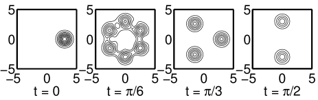
Figure 1: Time snapshots of Husimi $Q$-function for the initial coherent state $|\alpha\rangle=|3\rangle$. Kerr parameter $G=1$, no loss $\gamma_{0}=0$ and no pump $p=0$.

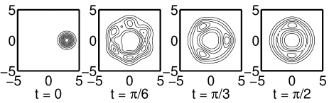
Figure 2: Same as in figure 1 but for the dissipative model with $\gamma_{0}=1$.

Obviously, the initial pure state remains pure ($E=L=0$).

IV.2 Dissipative non-linear oscillator without pump

When losses are involved in the system without a pump, the evolution is no more periodic and it ends in the vacuum state. During the time evolution, an initial state goes through various nonclassical states and through strongly mixed states. Some analytical solutions of the dissipative Kerr non-linear oscillator have been obtained both for ’quiet’ ($T\approx 0$) solution0 and ‘noisy’ ($T>0$) solution1 reservoirs.

The role of dissipation is clearly seen by comparing the evolution of the initial coherent state $|\alpha=3\rangle$ without (figure 1) and with (figure 2) losses. The parameters used in figures 1 and 2 are $G=1$, $p=0$ and the loss parameter $\gamma_{0}$ is 0 in figure 1 and $0.1$ in figure 2. Due to losses, no superpositions of coherent states arise in the evolution presented in figure 2. The effect can be explained as a fast destruction of internal coherence.

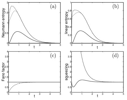
Figure 3: Evolution of the mixedness and noise for the system without a pump: (a) the von Neumann entropy $E$, (b) linear entropy $L$, (c) Fano factor $F$ and (d) squeezing parameter $S$ for the initial coherent state $|\alpha=3\rangle$ (thick solid curves), the Fock state $|n=9\rangle$ (dashed curves) and the superposition of three coherent states $|\psi_{3}\rangle$ (thin solid curves). Resonator parameters are $p=0$, $G=0.2$ and $\gamma_{0}=1$.

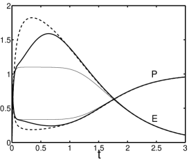
Figure 4: Evolution of the purity $P$ and entropy $E$ for the initial Fock state $|n=9\rangle$ (dotted curve) and for the superposition of three coherent states $|\psi_{3}\rangle$ with Kerr (thick solid) and without Kerr (thin solid curves). The resonator parameters are same as in figure 3.

Now we will analyse the evolution of the mixedness, characterized by the von Neumann ($E$) and linear ($L$) entropies, and the noise in terms of the Fano factor $F$ and quadrature squeezing parameter $S$ given in figure 3 for the parameters $G=0.2$, $p=0$ and $\gamma_{0}=1$. First we focus on the evolution of the initial coherent state $|\alpha\rangle=|3\rangle$ depicted by thick solid curves in figure 3. As seen, the signal state is maximally mixed at the time $t\approx 0.87$ when the entropies reach the values of $E\approx 0.57$ [figure 3(a)] and $L\approx 0.31$ [figure 3(b)]. During the evolution, the photocount statistics of the initial coherent state remains Poissonian. It is a direct consequence of the fact that the diagonal terms of the density matrix keep the Poissonian character for all the times. It can be shown that it holds exactly that

$$p\left(n\right)=\exp\left(-\langle n\rangle\right)\frac{\langle n\rangle^{n}}{n!},$$ (28)

where $\langle n\rangle=|\alpha|^{2}\exp\left(-2\gamma_{0}t\right)$, which explains why the Fano factor remains constant and equal to one for all the times [see figure 3(c)]. On the other hand, the quadrature noise evolves leading to the maximum squeezing of $S\approx 0.52$ at the time $t\approx 0.18$. In figure 3, we have also presented by thin solid curves the evolutions of the mixedness and the noise of the initial superposition of three coherent states (Schrödinger kittens)

$$|\psi_{3}\rangle=N_{3}\left(|3\rangle+|3\mathrm{e}^{\mathrm{i}\frac{2\pi}{3}}\rangle+|3\mathrm{e}^{-\mathrm{i}\frac{2\pi}{3}}\rangle\right),$$ (29)

where $N_{3}$ is a normalization constant. One can observe a rapid increase in the mixedness measured by both $E$ in figure 3(a) and $L$ in figure 3(b) during a very short time interval $t<0.05$. It can be explained as a general effect of the coherence loss of quantum components of the superposition $|\psi_{3}\rangle$. In general, it can be shown that the superposition of three strong coherent states (normalized by $N\approx 1/\sqrt{3}$):

$$|\psi\rangle=N\left(|\alpha_{1}\rangle+|\alpha_{2}\rangle+|\alpha_{3}\rangle\right)$$ (30)

exponentially fast evolves into the mixed state

$$\hat{\rho}=N^{2}\left(|\alpha_{1}\rangle\langle\alpha_{1}|+|\alpha_{2}\rangle\langle\alpha_{2}|+|\alpha_{3}\rangle\langle\alpha_{3}|\right)$$ (31)

as a consequence of the reservoir influence. The characteristic time of the decoherence process between $|\alpha_{i}\rangle$ and $|\alpha_{k}\rangle$ ($i\neq k$ for $i,k=1,2,3$) can be estimated as

$$\tau_{ik}\approx\left(2\gamma_{0}|\alpha_{i}-\alpha_{k}|^{2}\right)^{-1}.$$ (32)

So for strong fields, the decoherence process is much faster than the dissipative process itself. The mixedness measured by the linear entropy increases to a value of $L=2/3$, while by the von Neumann entropy increases to $E=\ln 3\approx\allowbreak 1.10$. In our case of $|\psi_{3}\rangle$ the increase in the linear entropy can be approximated by

$$L\approx\frac{2}{3}\left[1-\exp\left(-6\gamma_{0}|\alpha|^{2}t\right)\right].$$ (33)

whose validity is verified by the results shown in figures 3(a,b) and 4. We note that a better agreement with the decoherence theory is achieved for the system when the Kerr non-linearity is switched off (corresponding to thin solid curves in figure 4) rather than is switched on (depicted by thick solid curves). For longer times, the noise dominates the process and the signal state turns into the vacuum state. Thus, the squeezing parameter evolves into the value of one as shown in figure 3(d). As for the initial coherent state, the Fano factor for the initial superposition state $|\psi_{3}\rangle$ remains unchanged and equal to unity [see figure 3(c)] during the evolution of the unpumped system for arbitrary values of the interaction $G$ and loss $\gamma_{0}$ parameters.

For the initial Fock states $|n=9\rangle$, a rapid increase in the mixedness can also be observed in figure 3(a,b) as depicted by dotted curves. For $t\approx 0.35$ we find the mixedness parameters to be $L\approx 0.8$ and $E\approx 1.8$. The mechanism of decoherence and increase in the mixedness differ from those for the initial superposition of coherent states. We can explain the observed values simply as follows: by solving directly the Schrödinger equation for the initial Fock state $|n\rangle$, we get a diagonal density matrix at time $t$ described by the binomial distribution

$$p\left(k\right)=\rho_{kk}={n\choose k}\left(\mathrm{e}^{-2\gamma_{0}t}\right)^{k}\left(1-\mathrm{e}^{-2\gamma_{0}t}\right)^{n-k},$$ (34)

which is surprisingly completely independent of the Kerr non-linearity $G$. The mixedness parameter $L=1-\sum p^{2}\left(k\right)$ sums up to an expression proportional to a hypergeometric function ${}_{2}F_{1}(-n,-n,1,x)$, which is difficult to handle. But we can easily calculate the variance

$$\overline{\Delta^{2}k}=n\left(\mathrm{e}^{-2\gamma_{0}t}\right)\left(1-\mathrm{e}^{-2\gamma_{0}t}\right)$$ (35)

which reaches a maximum at the time moment when $\mathrm{e}^{-2\gamma_{0}t}=1/2$. So we can estimate the searched maximum of the linear entropy $L$ at this moment. We have

$$L_{\max}\approx 1-\sum_{k=0}^{n}{n\choose k}^{2}2^{-2n}=1-\frac{(2n)!}{(2^{n}n!)^{2}}$$ (36)

and for large $n$ we get the following simple approximation

$$L_{\max}\approx 1-\frac{1}{\sqrt{\pi n}},$$ (37)

by applying the Stirling formula $n!\approx\sqrt{2\pi n}e^{-n}n^{n}$. Thus, we can analytically estimate the loss of purity for $n=9$ as $L_{\max}\approx 0.815$ according to (36) (or slightly less accurate as 0.812 according to (37)), which can be expected at the time $t\approx 0.347$. We can calculate the entropy of the state at the same time moment to get $E\approx\allowbreak 1.\,\allowbreak 823$. These estimations are in full agreement with the precise numerical results given in figure 5(a,b). Finally, we note that the squeezing parameter decreases from $S=19$, while the Fano factor increases from $F=0$ for the initial Fock state to reach the value of one for the vacuum state in the time limit.

IV.3 Dissipative non-linear oscillator with pump

Here, we will analyse the system with the classical pump switched on, for which the initial state finally evolves into a stationary non-vacuum state. Its properties are determined by the pump intensity $p$ and by the passive parameters $\gamma_{0}$ and $G$. We will study three typical evolutions for different initial fields including coherent states, Fock states and superpositions of three coherent states. Figure 5 shows the Wigner function evolution of the coherent initial state $|\alpha=3\rangle$, figure 6 shows the evolution of the Fock initial state $|n=9\rangle$ and figure 7 shows evolution of the superposition of three coherent states, given by (29), for the same resonator parameters $p=5$, $\gamma_{0}=1$ and $G=0.2$. All the three states have been selected to have the same initial energy $\langle n\rangle=9$ (in the last case approximately). Six time snapshots of the Wigner function of the signal state are presented for the time moments $t=0,1/3,2/3,1,5$ and for a very long time, practically corresponding to $\infty$. In figure 5, the coherent initial state rotates and evolves in a banana-shape state and finally ends in a steady state. In figure 6, the initial Fock state of a ring shape is deformed and squeezes before ending in a steady state. In figure 7, the initial superposition of the coherent states rotates, deforms and its components converge into the same steady state.

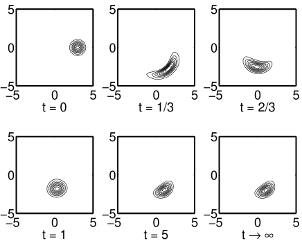
Figure 5: Time snapshots of Wigner function for the initial coherent state $|\alpha=3\rangle$. Resonator parameters are $G=0.2$, $\gamma_{0}=1$ and $p=5$.

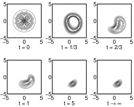
Figure 6: Same as in figure 5 but for the initial Fock state $|n=9\rangle$.

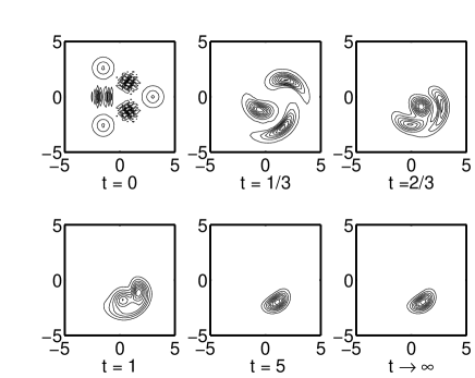
Figure 7: Same as in figure 5 but for the initial coherent state superposition $|\psi_{3}\rangle$.

Figure 8: Evolution of the mixedness and noise parameters same as in figure 4 but for the pumped system with $p=5$.

For the coherent initial state, the phase-space evolutions of the mean quantum $\langle\hat{a}(t)\rangle$ and classical $\alpha(t)$ amplitudes in the time interval $0<t<10$ are presented in figure 9. Both the spirals start at the point $\alpha=3$, and end at $\alpha\approx 1-2\mathrm{i}$. Note that the evolutions are very similar to each other even for the other times, which shows the validity of our semiclassical approximation.

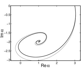
Figure 9: Phase space trajectory of quantum $\langle a\left(t\right)\rangle$ (thick curve) and classical $\alpha\left(t\right)$ (thin curve) solutions for $t\in\left(0,10\right)$.

The evolutions of the mixedness parameters $E$ and $L$ and the quantum noise parameters $F$ and $S$ for all the three initial states in the pumped system are depicted in figure 8. Note a rapid increase in the mixedness especially in the cases of the initial Fock state and a superposition of coherent states for very short evolution times, and then for longer times, a decrease in the mixedness for all the initial states. We observe that the evolutions for short times are similar to those presented in figure 3 for the unpumped system. However, for longer times (even for $t>5$ for the parameters of figure 8) all the three initial states of the pumped system evolve into some mixed steady state different from the vacuum state. This is in contrast to the evolution of the unpumped system for which $E(p=0)$ and $L(p=0)$ approach zero, while $S(p=0)$ and $F(p=0)$ approach one in the time limit (see figure 3), since the dissipative system without external pumping evolves into the vacuum state for any initial fields.

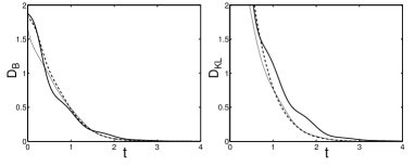
Figure 10: Evolution of the Bures metric ($D_{B}$) and the quantum relative entropy ($D_{K\!L}$) for the same initial states as in figure 8.

It is worth noting, although it is out of the focus of our interest, that the weakly-pumped non-linear oscillator ($p\ll G$) enables the so-called optical state truncation leonski and can be used for optical qubit generation.

IV.4 Steady-state solution

In figures 5–7 we have presented the evolutions of the Wigner functions up to the time $t=5$ and then checked for much longer times, practically, for $t\rightarrow\infty$. From this study we can conclude that all the three initial states end in the same steady state, which is centred around the same value of the complex amplitude $\alpha\approx 1-2\mathrm{i}$. All the other parameters studied that is: $E\approx 0.278$, $L\approx 0.135$, $\langle n\rangle\approx 5.13$, $F\approx 0.69$ and $S\approx 0.72$ of the steady state are the same as well. So, the steady-state solution is apparently unique and totally independent of the initial states. It can be therefore fully determined by the resonator parameters only. While for the system without a pump the evolution ends in the vacuum state, for the pumped system the asymptotic state is neither the vacuum nor pure, and can have intriguing noise properties. We can prove it by a decomposition of the steady-state density matrix in its spectrum of eigenstates.

Drummond and Walls found that no Glauber-Sudarshan $P$-function exists in the steady-state except as a generalized function drummond1 . The latter was used by Kheruntsyan to find the following explicit form of the steady-state density matrix kheru

$$\hat{\rho}_{\rm ss}=C\sum_{n,m}\frac{(\epsilon^{*})^{m}\epsilon^{n}}{\sqrt{m!n!}}\frac{{}_{0}F_{2}(\lambda^{\ast}+m,\lambda+n,|\epsilon|^{2})}{\Gamma(\lambda^{\ast}+m)\Gamma(\lambda+n)}|n\rangle\langle m|$$ (38)

where $C=\Gamma(\lambda^{\ast})\Gamma(\lambda)/_{0}F_{2}(\lambda^{\ast},\lambda,2|\epsilon|^{2})$, $\epsilon=-ip/G$, $\lambda=-i\gamma_{0}/G$, and ${}_{0}F_{2}$ is the generalized Gauss hypergeometric function. Eq. (38) readily enables calculation of the moments $\langle(\hat{a}^{{\dagger}})^{m}\hat{a}^{n}\rangle_{\rm ss}$ by the expressions summing up to

$$\langle(\hat{a}^{{\dagger}})^{m}\hat{a}^{n}\rangle_{\rm ss}=C(\epsilon^{*})^{m}\epsilon^{n}\,\frac{{}_{0}F_{2}(\lambda^{\ast}+m,\lambda+n,2|\epsilon|^{2})}{\Gamma(\lambda^{\ast}+m)\Gamma(\lambda+n)}$$ (39)

which corresponds to a slightly modified Drummond-Gardiner formula drummond2 . Solution (38), with the help of definition (11), also enables calculation of the steady-state Husimi and Wigner functions. E.g., the latter can be given by kheru

$${\cal W}^{(0)}_{\rm ss}(\beta)=N^{(0)}e^{-2|\beta|^{2}}\left|\frac{J_{\lambda-1}(\sqrt{-8\epsilon\beta^{\ast}})}{(\beta^{\ast})^{(\lambda-1)/2}}\right|^{2}$$ (40)

where $J_{\lambda-1}(x)$ is the Bessel function and $N^{(0)}$ is the normalization constant.

To find a physical insight of the steady-state density matrix (38), we rewrite it as the incoherent superposition (16):

$$\hat{\rho}_{\rm ss}=p_{0}|\psi_{0}\rangle\langle\psi_{0}|+p_{1}|\psi_{1}\rangle\langle\psi_{1}|+p_{2}|\psi_{2}\rangle\langle\psi_{2}|+...$$ (41)

of the orthogonal pure states $|\psi_{k}\rangle$ with the weight factors $p_{k}$, which can be found numerically. Applying the eigenvalue method for the steady state we have obtained all the spectrum of the final state. Wigner functions of the first three most important components are displayed in figure 11. The weight coefficients of the strongest components are in the sequence of $p_{0}\approx 0.928$, $p_{1}\approx 0.068$ and $p_{2}\approx 0.004$. The first component $|\psi_{0}\rangle$, apart from the second and third components, is strongly nonclassical with its quadrature noise of about $S_{0}\approx 0.60$, while the compound steady state has the quadrature noise level just about $S\approx 0.72$.

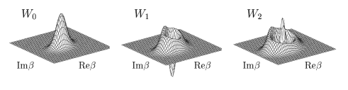
Figure 11: Wigner functions $W_{j}={\cal W}_{\rm ss}^{(0)}(|\psi_{j}\rangle)$ ($j=0,1,2$) of the first three pure state components of the steady state for the resonator parameters $G=0.2,\;p=5,\;\gamma_{0}=1$.

To verify the conclusion that the density matrices $\hat{\rho}(t)$ for different initial conditions evolve into the same steady state described by the density matrix (38), we calculate the Bures metric and the quantum relative entropy (the generalized Kullback-Leibler distance) between $\hat{\rho}(t)$ and $\hat{\rho}_{\rm ss}$ defined as follows vedral

$$D_{B}\{\hat{\rho}(t)||\hat{\rho}_{\rm ss}\} = 2-2\,{\rm Tr}\{[\sqrt{\hat{\rho}_{\rm ss}}\hat{\rho}(t)\sqrt{\hat{\rho}_{\rm ss}}]^{1/2}\},$$ (42)

$$D_{K\!L}\{\hat{\rho}(t)||\hat{\rho}_{\rm ss}\} = {\rm Tr}\{\hat{\rho}(t)[\ln\hat{\rho}(t)-\ln\hat{\rho}_{\rm ss}]\},$$ (43)

respectively. The square of trace in (42) is the so-called Uhlmann transition probability or the Jozsa fidelity for mixed states jozsa . Figure 10 clearly shows that the Bures metric and quantum relative entropy approach zero for the three different initial fields including coherent states, their superpositions and the Fock states.

In the next section we will show that the steady state can be well described as a nonclassical Gaussian state at least for high-pump intensities.

V Linearized approximation of the steady-state solution

Now we will give a linearized approximation of the steady-state solution of the Heisenberg equation (3). We start with the classical approximation for strong fields, when the quantum noise can be neglected and the signal mode can be described by a complex amplitude. Heisenberg equation (3) gives the following ordinary differential equation

$$\frac{\mathrm{d}\alpha}{\mathrm{d}t}=p-2\mathrm{i}G|\alpha|^{2}\alpha-\gamma_{0}\alpha$$ (44)

for the complex amplitude $\alpha$. Minor differences between the exact quantum mean amplitude $\langle a\left(t\right)\rangle$ and the classical amplitude $\alpha\left(t\right)$ for the coherent initial state $|\alpha=3\rangle$ and for the resonator parameters $p=5$, $G=0.2$ and $\gamma_{0}=1$ can be seen in the phase-space trajectory depicted in figure 9.

If we are interested in the steady-state solution only, we may replace the left hand side of equation (44) by zero and solve it. The complex equation can be transformed into the real equation

$$|p|^{2}=\left(\gamma_{0}^{2}+4G^{2}|\alpha|^{4}\right)|\alpha|^{2},$$ (45)

which is a cubic equation in intensity $|\alpha|^{2}$. A simple analysis shows that the amplitude $|\alpha|$ of the steady-state solution is a monotonic function of the pump parameter $|p|$ and so equation (45) has a unique solution and no threshold can be observed. Since the explicit form of the solution is too complex to find some relevant physics in it, we will not present it here. We note only that for the resonator parameters $p=5$, $G=0.2$ and $\gamma_{0}=1$ assumed in the examples investigated in the previous section one can find the exact classical steady-state solution $\allowbreak|\alpha|^{2}=5$ and $\alpha=1-2\mathrm{i}$. In particular, (i) for $p=0$, equation (45) has a trivial solution of $\alpha=0$, (ii) for weak pump $|p|^{2}\ll\gamma_{0}^{3}/2G$, the amplitude grows linearly with the pump intensity as $\alpha\approx p/\gamma_{0}$ and (iii) for very strong pump $|p|^{2}\gg\gamma_{0}^{3}/2G$, the amplitude grows with the third root of the pump intensity

$$\alpha\approx-\mathrm{i}\frac{p}{|p|}\left(\frac{|p|}{2G}\right)^{1/3}.$$ (46)

To describe the noise properties of the signal mode we will search a solution to equation (3) as a sum of two components $\hat{a}=\alpha+\hat{A}$, where $\alpha$ is the strong classical complex amplitude and $\hat{A}$ is the weak quantum noise operator. By inserting it into equation (3) and after linearization one gets the following equation for the noise operator

$$\frac{\mathrm{d}\hat{A}}{\mathrm{d}t}=-\gamma\hat{A}-\delta\hat{A}^{{\dagger}}+\hat{\cal L},$$ (47)

where the complex coefficients $\gamma$ and $\delta$ depend on time through the amplitude $\alpha$ and are given by the relations

$$\gamma=\gamma_{0}+4\mathrm{i}G|\alpha|^{2},\qquad\delta=2\mathrm{i}G\alpha^{2}.$$ (48)

The solution of equation (47) is a Gaussian state, defined by (54) in Appendix A, exhibiting purely nonclassical properties, thus referred to as the NCGS. The time evolution of the NCGS parameters $B$ and $C$ is described by the two differential equations

$$\dot{B} = -2\left(\gamma+\gamma^{\ast}\right)B-\left(\delta^{\ast}C+\delta C^{\ast}\right),$$

$$\dot{C} = -\delta\left(1+2B\right)-2\gamma C.$$ (49)

From them one can obtain numerically the linearized solution of the Heisenberg equation (3), but it is meaningless when we know the exact quantum solution. Instead of that we will focus on the steady-state solution only. Since $|\gamma|>|\delta|$, a stationary solution of the operator equation (47) exists. It is the NCGS with the following parameters bajer2

$$2B=\frac{|\delta|^{2}}{|\gamma|^{2}-|\delta|^{2}},\qquad 2C=-\frac{\delta\gamma^{\ast}}{|\gamma|^{2}-|\delta|^{2}}.$$ (50)

Since we know all the three parameters $\alpha$, $B$ and $C$ of the NCGS, we can simply estimate the other parameters of the steady state, where the corresponding formulas are given in Appendix A. For example, for the quadrature noise squeezing parameter (59) one can derive a simple formula

$$S=\frac{|\gamma|}{|\gamma|+|\delta|}\leq 1$$ (51)

demonstrating that the steady state is squeezed. The parameter $x$, defined by (56), is explicitly given by

$$x=\frac{1}{2}\left(\sqrt{\frac{|\gamma|^{2}}{|\gamma|^{2}-|\delta|^{2}}}-1\right).$$ (52)

Numerically, for the resonator parameters $p=5$, $G=0.2$ and $\gamma_{0}=1$, we get $\alpha=1-2\mathrm{i}$, $\gamma=1+4\mathrm{i}$, $\delta=1.\,\allowbreak 6-1.\,\allowbreak 2\mathrm{i}$, $S\approx 0.673$, $F\approx 0.711$, $x\approx 0.072$, $p_{0}\approx 0.933\,$, $p_{1}\approx 0.06\allowbreak 2$ and $p_{2}\approx\allowbreak 0.004$. From formula (58) we estimate the linear entropy of the steady state as $L\approx 0.126$ and from (57) we estimate the von Neumann entropy as $E\approx 0.263$. Surprisingly, these estimations match the exact values already for relatively low pump intensities. For higher pump intensities the agreement is even better.

Note that in the strong pump approximation, a very simple relation holds $|\gamma|=2|\delta|$, which gives crude estimations of $S=2/3$ and $F=2/3$. Since $x=\frac{1}{3}\sqrt{3}-\frac{1}{2}\approx 0.0774$, the linear entropy is estimated as $L=1-\sqrt{3}/2\approx 0.134$ and the entropy as $E\approx 0.278$. We can also estimate the weight coefficients of steady state decomposition as $p_{0}\approx 0.928$, $p_{1}\approx 0.067$, $p_{2}\approx 0.005$. So, even the crude estimations well match the exact values obtained numerically in the previous section.

In figure 12 we have compared the exact quantum weight factors $p_{k}$ of the steady state and the approximate Gaussian weight factors given by (55) with $x\approx 0.072$ calculated from (56) for the resonator parameters $G=0.2,$ $\gamma_{0}=1$ and $p=5$. This graphical representation shows the validity of our approximation.

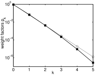
Figure 12: Exact quantum weight factors $p_{k}$ of the steady state (thick curve with squares) vs the Gaussian state approximation given by (55) (thin curve with circles)

VI Conclusions

We studied the evolution of the quantum noise and mixedness of a dissipative non-linear oscillator, described by a Kerr non-linear oscillator, pumped by a classical external field. We quantified the quantum noise by the quadrature squeezing parameter and the Fano factor, while the mixedness by the quantum von Neumann and linear entropies. Dissipation was described in the standard Heisenberg-Langevin approach by coupling the system to zero-temperature reservoir. We demonstrated that initial pure states, including the Fock states, coherent states, and their finite superpositions, exhibited fast decoherence and evolved into the same steady mixed state being well approximated by a nonclassical Gaussian state as verified by the Bures metric and the quantum relative entropy. We presented analytical formulas and numerical results for the steady state parameters to show that the state exhibits quadrature noise squeezing and sub-Poissonian statistics if the thermal reservoir is cold. We observed, especially for the initial nonclassical states including the Fock states or the finite superpositions of coherent states, a rapid increase in the mixedness at the very beginning of the evolution, and then for longer times a fall in the mixedness to the same low value of the asymptotic nonclassical Gaussian state in the case of the cold reservoir.

Appendix A Gaussian states

The Gaussian state is defined as a state with Gaussian quasidistribution and Gaussian characteristic functions (see, e.g., perina ; perinova ; paris ), which can be identified completely by the three parameters

$$\alpha=\langle\hat{a}\rangle,\;\;\;\;\;B=\langle\hat{a}^{{\dagger}}\hat{a}\rangle-\langle\hat{a}^{{\dagger}}\rangle\langle\hat{a}\rangle,\quad C=\langle\hat{a}^{2}\rangle-\langle\hat{a}\rangle^{2}.$$ (53)

Thus the Gaussian state can be defined by its Cahill-Glauber $s$-parametrized quasidistribution function

$${\cal W}^{(s)}(\beta) = \frac{1}{\pi\sqrt{K_{s}}}\exp\Big{(}-\frac{1-s+2B}{2K_{s}}|\beta-\alpha|^{2}$$ (54)

$$\hskip 28.45274pt+\left[\frac{C^{\ast}}{K_{s}}\left(\beta-\alpha\right)^{2}+\mathrm{c.c.}\right]\Big{)},$$

where $K_{s}=\left(1/2-s/2+B\right)^{2}-|C|^{2}$. The Gaussian state is a natural generalization of coherent ($B=C=0$) and chaotic ($C=0$) states. Note that in a special case of $s=1$, the Glauber-Sudarshan function $P(\beta)\equiv{\cal W}^{(1)}(\beta)$ exists if $K_{1}>0$, otherwise the state described by (54) is nonclassical, and thus referred to as the NCGS. The Gaussian states are mixed states with the weight coefficients

$$p_{k}=\frac{x^{k}}{\left(1+x\right)^{1+k}},$$ (55)

where

$$x=\sqrt{\left(B+\frac{1}{2}\right)^{2}-|C|^{2}}-\frac{1}{2}.$$ (56)

The von Neumann entropy of the Gaussian state (54) reads as perinova

$$E=-\ln\frac{x^{x}}{\left(1+x\right)^{1+x}}$$ (57)

Similarly, it is easy to show that the purity parameter is

$$P=(1+2x)^{-1},$$ (58)

while the quadrature noise squeezing parameter reads as

$$S=1+2(B-|C|)$$ (59)

and its Fano factor is

$$F=1+2B+\frac{C\alpha^{\ast 2}+C^{\ast}\alpha^{2}}{|\alpha|^{2}+B},$$ (60)

where the parameters $\alpha$, $B$ and $C$ are defined by (53). Note that the squeezing occurs if $B<|C|$ or equivalently if $K_{1}<0$, so any NCGS exhibits quadrature squeezing.

References

- (1) von Neumann J 1955 Mathematical Foundations of Quantum Mechanics (New York: Princeton University Press)
- (2) Drummond P D and Walls D F 1980 J. Phys. A 13 725
- (3) Drummond P D and Gardiner C M 1980 J. Phys. A 13 2353
- (4) Kheruntsyan K V 1999 J. Opt. B: Quantum Semiclass. Opt. 1 225
- (5) Peřina J 1991 Quantum Statistics of Linear and Nonlinear Optical Phenomena (Dordrecht: Kluwer) p 185
- (6) Cahill K E and Glauber R J 1969 Phys. Rev. 177 1857
- (7) Tanaś R, Miranowicz A and Gantsog Ts 1996 Progress in Optics vol 35, ed E Wolf (Amsterdam: North-Holland) p 355
- (8) Życzkowski K, Horodecki P, Sanpera A and Lewenstein M 1998 Phys. Rev. A 58 883
- (9) Kitagawa M and Yamamoto Y 1986 Phys. Rev. A 34 3974
- (10) [] Milburn G J 1986 Phys. Rev. A 33 674
- (11) [] Tanaś R and Kielich S 1983 Opt. Commun. 45 351
- (12) Bajer J, Miranowicz A, and Tanaś R 2002 Czech. J. Phys. 52 1313
- (13) Yurke B and Stoler D 1986 Phys. Rev. Lett. 57 13
- (14) [] Mecozzi A and Tombesi P 1987 Phys. Rev. Lett. 58 1055
- (15) Miranowicz A, Tanaś R, and Kielich S 1990 Quantum Opt. 2 253
- (16) Milburn G J and Holmes C A 1986 Phys. Rev. Lett. 56 2237
- (17) [] Peřinová V and Lukš A 1988 J. Mod. Opt. 35 1513
- (18) Daniel D J and Milburn G J 1989 Phys. Rev. A 39 4628
- (19) [] Peřinová V and Lukš A 1990 Phys. Rev. A 41 414
- (20) [] Chaturvedi S and Srinivasan V 1991 J. Mod. Opt. 38 777
- (21) Leoński W 1996 Phys. Rev. A 54 3369
- (22) [] Leoński W and Miranowicz A 2001 Adv. Chem. Phys. (New York: Wiley) 119(I) 195
- (23) Vedral V, Plenio M B, Rippin M A, and Knight P L 1997 Phys. Rev. Lett. 78 2275
- (24) Jozsa R 1994 J. Mod. Opt. 41 2315
- (25) Bajer J 1991 J. Mod. Opt. 38 1085
- (26) Peřinová V, Křepelka J, Peřina J, Lukš A, and Szlachetka P 1986 Optica Acta 33 15
- (27) Paris M G A, Illuminati F, Serafini A and De Siena S 2003 Phys. Rev. A 68 012314