Entanglement in a two-qubit Ising model under a site-dependent external magnetic field

Abstract

We investigate the ground state and the thermal entanglement in the two-qubit Ising model interacting with a site-dependent magnetic field. The degree of entanglement is measured by calculating the concurrence. For zero temperature and for certain direction of the applied magnetic field, the quantum phase transition observed under a uniform external magnetic field disappears once a very small non-uniformity is introduced. Furthermore, we have shown analytically and confirmed numerically that once the direction of one of the magnetic field is along the Ising axis then no entangled states can be produced, independently of the degree of non-uniformity of the magnetic fields on each site.

I INTRODUCTION

The existence of entangled states of component systems and their unique properties have attracted a lot of attention since the early days of quantum mechanics [1-5]. Entanglement has also recently been the subject of several investigations as it plays an important role in the topical areas of quantum computation and quantum information processing [6,7].

The Heisenberg magnetic spin system is one of the few physical systems that entanglement arise naturally. Nielsen [7] was the first to report results on entangled states utilized in a two-spin system. He calculated the entanglement of formation of a magnetic system described by an isotropic XXX Heisenberg Hamiltonian in an external magnetic field directed along the z-axis. Later, Arnesen et al. [8] systematically investigated the dependence of entanglement on temperature and on the applied external field in the same 1D Heisenberg system. They showed that for ferromagnets the spins are always disentangled while entanglement is observed for antiferromagnets. In addition, they found that the degree of entanglement can be enhanced by increasing the external parameters (magnetic field and/or temperature). Then, Wang [9,10] studied the effect of anisotropy on thermal entanglement, working on the two-qubit quantum anisotropic Heisenberg XY model [9] and on the anisotropic Heisenberg XXZ model [10]. He also investigated the isotropic Heisenberg XX model with an external magnetic field applied along the $z$-axis [9]. Kamta and Starace [11] investigated the thermal entanglement of a two-qubit Heisenberg XY chain in the presence of an external magnetic field along the $z$-axis. They showed that by adjusting the magnetic field strength, entangled states are produced for any finite temperature. Sun et al. [12] extended later the work reported in Ref. [11] by introducing a non-uniform magnetic field. Comparing to the uniform field case, they showed that entanglement can be more effectively controlled via a non-uniform magnetic field. The full anisotropic XYZ Heisenberg spin two-qubit system in which a magnetic field is applied along the $z$-axis, was studied by Zhou et al. [13]. The enhancement of the entanglement for particular fixed magnetic field by increasing the $z$-component of the coupling coefficient between the neighboring spins, was their main finding. Finally, thermal entanglement in a two-qubit Ising model assuming an applied magnetic field in an arbitrary direction has been investigated by Gunlycke et al. [14].

Several, mainly numerical, works exist also on the study of pairwise thermal entanglement in the $n$-qubit Heisenberg spin chain. In short, the systems being studied are the XXZ three-qubit Heisenberg model with an applied magnetic field in the $z-$ direction [15], the XYZ three-qubit Heisenberg model with an applied magnetic field along the $z$-axis [13], the XX four-qubit Heisenberg model with an applied magnetic field in the $z$-direction [16], the XX [17] and XXX and XXZ [18] four- and five-qubit Heisenberg model and the XX $m$-qubit (with $m$ up to eleven) Heisenberg model [19].

It turns to be quite interesting to study the general case of different magnetic fields at each spin site. The control of the applied field at each spin separately is very useful in order to perform quantum computations [20]. Hence in the present theoretical analysis we investigate the ground state and the thermal entanglement in an Ising model with a non-uniform and anisotropic external magnetic field, i.e. the magnitude and the direction of each magnetic field is different in each spin.

This article is organized as follows: In the following section we present the details of the theoretical analysis based on the calculation of the concurrence [21,22] of the system. Then, in section III numerical results are presented and discussed for several cases of the parameters of the system (magnetic fields magnitudes and directions and temperature). In addition, a general analytical result is presented in the Appendix. There, we show that once one of the applied external magnetic fields points along the Ising direction, no matter what is the direction and magnitude of the other field the concurrence is always zero. This result is valid for zero and finite temperatures. Our results are summarized in section IV.

II THEORY

The Hamiltonian studied in this work is given by

$$H=J(\sigma_{1}^{z}\sigma_{2}^{z}+\sigma_{2}^{z}\sigma_{1}^{z})+B_{1}\cos\theta_{1}\sigma_{1}^{z}+B_{1}\sin\theta_{1}\sigma_{1}^{x}+B_{2}\cos\theta_{2}\sigma_{2}^{z}+B_{2}\sin\theta_{2}\sigma_{2}^{x}\quad,$$ (1)

where $\sigma^{a}$ are the Pauli operators and $J$ is the strength of the Ising interaction. Also, $B_{1}$ and $B_{2}$ are the magnitudes of the external magnetic fields. We assume that each magnetic field has an arbitrary direction, defined by the angles $\theta_{1}$ and $\theta_{2}$ between the field and the Ising direction. It is sufficient to consider that the magnetic field lies in a plane (xz) containing the Ising $z$-direction, because in three spatial dimensions, the Hamiltonian possesses rotational symmetry about the $z$-axis.

A useful and convenient quantitative tool, which has been developed to study entanglement, is the entanglement of formation [4]. The entanglement of formation of a state of a composite system is proportional to the minimum number of Bell states, which must be shared between the components of the composite system. There is no general prescription for evaluation of the entanglement of formation in arbitrary systems. In this area Wootters [21] has described an explicit method for evaluating the entanglement of formation of an arbitrary state of a two-qubit system. His explicit formula is a generalization of the expression derived by him and Hill [22] for a special class of density matrices.

For a pair of qubits the entanglement of formation $E_{12}$ is estimated from the expression $E_{12}=h\left({1+\sqrt{1-C_{12}^{2}}}\right)/2$, where $C_{12}$ denotes the concurrence and $h$ is the binary entropy function [21]. The concurrence is defined as $C_{12}=\max\{\lambda_{1}-\lambda_{2}-\lambda_{3}-\lambda_{4},0\}$, where the $\lambda$’s are the square roots of the eigenvalues in decreasing order of magnitude (i.e. $\lambda_{1}\geq\lambda_{2}\geq\lambda_{3}\geq\lambda_{4})$ of the spin-flipped density matrix operator $R_{12}=\rho(\sigma^{y}\otimes\sigma^{y})\rho\ast(\sigma^{y}\otimes\sigma^{y})$. Here, $\rho$ is the density matrix operator defined as $\rho=\exp(-H/k_{B}T)/Z$, where $Z$ is the partition function ($Z=tr\{\exp(-H/k_{B}T)\})$ and $k_{B}$ is the Boltzmann’s factor. As concurrence is a monotonically increasing function of $E_{12}$ and both functions have values in the range 0 to 1, we practically use $C_{12}$ as a measure of the entanglement. Zero concurrence corresponds to an un-entangled pair of states and unity concurrence to a maximally entangled pair of states. This type of entanglement is usually called thermal entanglement as it is described by a temperature dependent density matrix operator.

In order to proceed we need to find the eigenvalues ($E_{i})$ and eigenvectors ($\left|{\Psi_{i}}\right\rangle)$ of the Hamiltonian of the Ising system in the presence of a non-uniform external magnetic field, i.e. the Hamiltonian of Eq. (1). Once we have determined the eigenstates of the system, the density matrix operator can be written as

$$\rho=Z^{-1}\sum\limits_{i}{\exp(-E_{i}/k_{B}T)}\left|{\Psi_{i}}\right\rangle\left\langle{\Psi_{i}}\right|\quad.$$ (2)

Then, the spin-flipped matrix operator is evaluated in a $4\times 4$ matrix representation, in terms of the natural basis vectors $\{\left|{00}\right\rangle,\left|{01}\right\rangle,\left|{10}\right\rangle,\left|{11}\right\rangle\}$. In most cases, even if one obtains analytic expressions for the eigenvalues of the spin-flipped matrix operator, it is practically impossible to derive a simple analytic expression for the concurrence. The reason lies to the fact that the relative order of magnitude of the eigenvalues of $R_{12,}$ depends on the parameters involved. In general the concurrence can be evaluated numerically. For particular values of the parameters of the system, an analytic expression can be achieved (see in the Appendix). It is worth pointing out that the above analysis is greatly simplified for the zero temperature case, and then only the ground state is populated and hence $\rho=\left|{\Psi_{0}}\right\rangle\left\langle{\Psi_{0}}\right|$, where 0 is the index that denotes the ground state of the system.

III RESULTS AND DISCUSSION

We begin our discussion with the results of the ground state of the system at zero absolute temperature $\left({T=0}\right)$. In Fig. 1(a) we assume a uniform magnetic field (i.e. same magnitude and same direction of magnetic field in each spin) and present the results of the concurrence as a function of the strength of the applied fields. It is clear that the entanglement is highest for nearly vanishing magnetic fields and decreases with increasing the field’s amplitude. In this figure we observe that for $B_{1}=B_{2}=B\to 0^{+}$, the concurrence is unity, which shows the creation of maximally entangled states. Once we set a zero value for the magnetic field, the eigenstates are the same as those of the Ising model without magnetic field, i.e. the standard disentangled basis $\{\left|{00}\right\rangle,\left|{01}\right\rangle,\left|{10}\right\rangle,\left|{11}\right\rangle\}$, as the Hamiltonian is diagonal in this basis. Therefore, the concurrence obtains a zero value. Then, even for an infinitesimal increase of the magnetic field, the system goes from a non-entangled state to a maximally entangled state. This is a clear evidence of a quantum phase transition (QPT) [23]. In the case that the magnetic field is along the $z$-axis, so that $\theta_{1}=\theta_{2}=0$, we have no entanglement at all. In this case the ground state has energy –2$J$ and is doubly degenerate. For small, but equal, angles $\theta_{1}=\theta_{2}$, there are two energy levels, one of energy value –2$J$ and the other with energy close to –2$J$, with corresponding states, the first one equal to the Bell state $\left({\left|{01}\right\rangle-\left|{10}\right\rangle}\right)/\sqrt{2}$ and the other close to the Bell state $\left({\left|{01}\right\rangle+\left|{10}\right\rangle}\right)/\sqrt{2}$. Thus, we get a maximally entangled qubit pair. Hence, we conclude that even a very small component of the magnetic field along the $x$-axis is adequate to create entangled states. In all cases we observe that the concurrence drops to zero for very strong fields. This is expected as for very strong fields the spins will be completely aligned along the field direction and hence the entanglement will drop to zero. It is worth noting that the smaller the $x$-component of the magnetic field becomes, the faster the concurrence drops to zero for $B>2J$. In the case where the magnetic field is along the $x$-axis the concurrence can be calculated analytically from the density matrix of the pure (ground) state, and we get $C_{12}=\left[{1+\left({B\mathord{\left/{\vphantom{BJ}}\right.\kern-1.2pt}J}\right)^{2}}\right]^{-1/2}$, see short dashed line ($\theta_{1}=\theta_{2}=\pi/2)$ in Fig. 1(a). The physical explanation of this behavior comes from the fact that the field tends to align the qubit spins in a different disentangled state from the spin-spin coupling. This implies that it is the trade off between the field and the Ising interaction that produces the entanglement.

We now investigate the case of non-uniform magnetic field, which is actually more realistic than the uniform magnetic field case. In Fig. 1(b) we observe that for $B_{2}$ slightly different from $B_{1}$ (here, $B_{2}=1.0005[B_{1}\equiv B])$ the QPT disappears in cases of small $x$-component of the magnetic fields. Now the concurrence starts from vanishing value reach a maximum value for $B<2J$ and then drops to zero very abruptly for $B>2J$. For small, but equal, angles $\theta_{1}=\theta_{2}$, there are two energy levels one of energy value –2$J$ and the other with energy value close to –2$J$but in this case the corresponding states are not close to the Bell states $\left({\left|{01}\right\rangle\pm\left|{10}\right\rangle}\right)/\sqrt{2}$. As the $x$-component of the magnetic field increases the change from the vanishing value of the concurrence at zero field is very abrupt, as can be seen from the short dashed curve ($\theta_{1}=\theta_{2}=\pi/2)$ in Fig. 1(b). For example, for $\theta_{1}=\theta_{2}=0.3\pi$ and for a magnetic field of value $B=$0.01$J$ the concurrence is practically unity. A very similar behavior is observed for slightly different directions of the magnetic fields $B_{1}$and $B_{2}$, as can be seen in Fig.1(c). In this case, we observe that the QPT disappears for magnetic fields of the same magnitude but slightly different direction. It is important to point out that this phenomenon is present even for directions of the magnetic fields very close to the $x$-direction. Again, we get that there are two lowest energy levels corresponding to states that are not close to the Bell states $\left({\left|{01}\right\rangle\pm\left|{10}\right\rangle}\right)/\sqrt{2}$. For larger differences between the magnitudes of the magnetic fields for the two qubits, i.e. $B_{2}=1.05B_{1}$, the disappearance of the QPT is even more pronounced for cases characterized by small $x$-component of the magnetic fields [see solid curve in Fig. 1(d)]. A systematic study of the field effects is depicted in Fig.2, where we plot the concurrence for cases of small [Figs. 2(a) and (b)] and large [Figs. 2(c) and (d)] difference in the magnetic field magnitude. We observe that the entanglement achieved for low $B_{x}$ components is the one that it is more influenced. For example, even for a very small difference in the field amplitudes (of the order of 1.05) the maximum entanglement is diminished. For a larger value of the amplitudes of the field ratio, e.g. for 1.5, the concurrence practically disappears (not shown). The reason for this behavior is due to the fact that the eigenvectors are in this case the non-entangled pure states $\left|{01}\right\rangle,\left|{10}\right\rangle$ and $\left|{00}\right\rangle$. As we see from the same figure, the influence of the non-uniformity of the magnetic fields becomes smaller the more the direction of the fields get closer to a direction along the $x$-axis. In the same figure we investigate the influence of the difference in the field directions. We note that the maximum change in the behavior is obtained for the case that $B_{x}$ is small.

We will now study the case of finite temperature, i.e. the case of thermal entanglement. We examine how the effects discussed in Fig. 1(a) changes for two different values of temperature with $B_{1}=B_{2}(=B)$, $\theta_{1}=\theta_{2}$. From Figs. 3 and 4 we clearly see that the critical temperature depends on the orientation of the fields and that the field at which the maximum entanglement occurs as the temperature increases shifts to larger values of the magnetic field amplitudes. First, we study the case of the low $B_{x}$ component, where we observe a sharp peak in the concurrence. We note there is a fast drop of the concurrence to zero for a low $B_{x}$ component and for low values of the field magnitude. The behavior found in Figs 3 and 4 has already reported and discussed in Ref. [14]. From the same plots we observe that as the direction of the fields gets close to an orthogonal direction with respect to the Ising axis, the maximum entanglement occurs at lower values of the magnetic filed magnitude. In the case of $\theta=\pi/2$, the concurrence does not drop to zero very fast as the eigenvectors of all eigenstates are either Bell states or a linear combination of Bell states.

Comparing Fig. 1(a) and Fig. 3(a), we clearly see that the QPT is not present in the finite temperature case. Moreover, we perform calculations for finite temperature with magnetic fields the same as those in Figs 1(b) and 1(c). We have found that for these values of the external parameters, the concurrence is practically the same as in Fig.3(a). This finding is valid once the magnitudes of the two applied fields are very similar. For case of larger difference in the field magnitude, the finite temperature results are more influenced as one sees by comparing Fig.1(d) and Fig.3(b). In this case of finite temperature under higher anisotropy of fields the QPT disappears, independently of the direction of the applied fields. Another, general feature seen from Fig. 4 (in comparison to Fig. 2) is that in all the cases the finite temperature leads to a decrease in the concurrence and shifts the maximum value of the concurrence at stronger applied fields. The effect is more pronounced for directions of the fields along an axis perpendicular to the Ising axis.

It is known [14] that there is an angle $\theta_{1}=\theta_{2}=\theta\left({B,T}\right)$ where the entanglement is maximum for a given temperature and amplitude ($B_{1}=B_{2})$. This feature, known as the phenomenon of magnetically induced entanglement, has been explained heuristically assuming that with $B_{x}$ and $B_{z}$ fixed, the entanglement should change continuously with temperature. As the increase in the temperature widens the low-entanglement zone around $B_{x}=0$ [14] and the entanglement has to fall for large $B_{x}$, it is expected that at some intermediate value of $B_{x}$, the maximal entanglement will be reached. The preferred angle traverses from $\theta=0$ at zero temperature to $\theta=\pi/2$ at $T\sim J/k_{B}$. First, we investigate the zero temperature case. For parallel directions of the magnetic fields, the maximum concurrence is achieved for fields pointing along the $x$-axis (not shown here). Moreover, we observe that once we fix the direction of one of the applied fields the direction of the field applied at the other spin depends on the relative magnitude of the fields. This dependence is minimal once one of the fields is along the $x$-axis (not shown here). We note that there is a cutoff value of the magnetic field magnitude applied on the second spin, above which the relative angle remains practically the same. This cutoff value depends on the direction of the magnetic field applied at the first of the spins. We have shown that for non-uniform fields ($B_{1}=J,\mbox{ }B_{2}=1.5J)$ the maximum concurrence is obtained for non-parallel directions of the two applied fields. We observe that the smaller the $B_{x}$ component of one of the fields becomes the more the system deviates from the parallel direction. Actually, we have found that for fields of equal magnitudes and smaller than $2J$, no matter what is the direction of the field applied at the first spin, the maximum concurrence is achieved for magnetic field at the second spin pointing at the same direction as in the first one. This is not true for fields of equal magnitudes but with values larger than $2J$. The deviation from parallel fields becomes more pronounced the more the direction of one of the fields gets closer to the Ising direction. It is well understood that if both fields get very large values the concurrence is zero. In our study we found that there is no entanglement even if either one of the fields is very large. How large should the field be in order to destroy entanglement depends on the orientations of the fields. A rule of thumb is that we need larger fields as the directions of the fields gets closer to a direction perpendicular to the Ising direction.

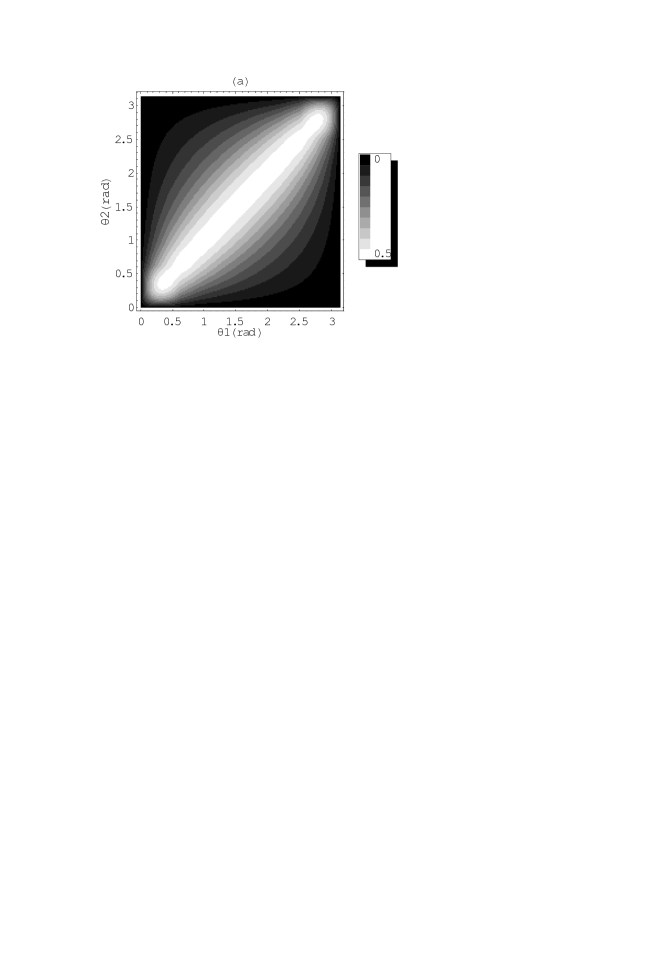
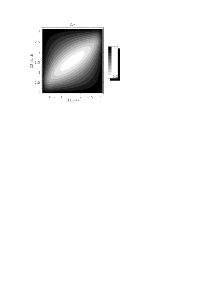
Figure 5: Contour plots of concurrence as a function of the directions of magnetic fields $\theta_{1}$ and $\theta_{2}$ (polar angles between field and Ising $z$-axis) for zero temperature. In both plots $B_{1}$=2.1$J$. In (a) $B_{2}=B_{1}$ and in (b) $B_{2}$=3$B_{1}$.

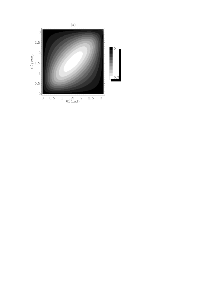
Figure 6: Contour plots of concurrence as a function of the directions of magnetic fields $\theta_{1}$ and $\theta_{2}$. In both plots $T$= 1$J$/$k_{B}$ and $B_{1}$=2.1$J$. In (a) $B_{2}=B_{1}$ and in (b) $B_{2}$=3$B_{1}$.

In Fig. 5(a) we confirm that for fields of equal magnitude ($B_{1}=B_{2})$, the maximum concurrence occurs for $\theta_{1}=\theta_{2}$. On the contrary, Fig. 5(b) shows that for non-uniform fields the maximum entanglement occurs for unequal angles ($\theta_{1}\neq\theta_{2})$. Actually, as the difference in the magnitude of the two fields increases, the maximum entanglement occurs for direction of the larger field along the $x$-axis independent of the direction of the other field. A very similar behavior was found for a finite temperature as shown in Fig.6.

IV CONCLUSIONS

In summary, in the present work, a systematic investigation was performed on the entanglement in a two-spin Ising model in a site-dependent magnetic field. One of the most interesting results is the finding that the QPT observed at zero temperature when a uniform magnetic field is applied, disappears with the introduction of a very small difference in the applied fields. This difference could be either a difference in magnitude or a difference in the direction of the magnetic fields. Moreover, we have found that for parallel fields with direction close to the $z$-axis (Ising direction), small differences in the magnetic field magnitudes result in very weak entanglement. On the contrary, a very large asymmetry in the amplitudes of the applied fields has small effects on the well-entangled states obtained for fields with large $x$-component. We have also studied the phenomenon of the magnetically induced entanglement and observe that for equal magnitudes of the external magnetic fields the maximum concurrence occurs for parallel directions of the fields. Once a non-uniformity is introduced the maximally entangled states obtained for non-parallel orientations of the fields. In addition, we have shown that the concurrence drops to zero even if only one of the fields gets very large values. Finally, we have derived an analytic result valid for ground state entanglement and thermal entanglement. The analytic result, which has been confirmed numerically, predicts that we get vanishing concurrence once the direction of one of the fields is along the Ising direction.

APPENDIX

In the Appendix we discuss the special case of one magnetic field parallel to $z$-azis and the other in any direction. We find analytic expressions that predict that the concurrence in this case is always zero. The Hamiltonian studied in this case is given by

$$H=J(\sigma_{1}^{z}\sigma_{2}^{z}+\sigma_{2}^{z}\sigma_{1}^{z})+B_{1}\sigma_{1}^{z}+B_{2}\cos\theta\sigma_{2}^{z}+B_{2}\sin\theta\left({\sigma_{1}^{+}+\sigma_{1}^{-}}\right)/2\quad,$$ (3)

where $\sigma^{a}$ are the Pauli operators and $J$ is the strength of the Ising interaction. Also, $B_{1}$ and $B_{2}$ are the magnitudes of the external magnetic fields. We assume that the first spin feels a magnetic field along the $z$-direction and the second field has an arbitrary direction, defined by the angle $\theta$ between the field and the Ising direction.

The eigenenergies and the eigenstates can be calculated analytically. The eigenenergies are:

$$E_{\pm}^{X} = -B_{1}\pm\left[{4J^{2}+B_{2}^{2}-4JB_{2}\cos\theta}\right]^{1/2}\,,$$ (4)

$$E_{\pm}^{Y} = B_{1}\pm\left[{4J^{2}+B_{2}^{2}+4JB_{2}\cos\theta}\right]^{1/2}\,,$$ (5)

The corresponding normalized eigenvectors are

$$\left|{X_{\pm}}\right\rangle = a_{\pm}\left|{00}\right\rangle+b_{\pm}\left|{01}\right\rangle\,,$$ (6)

$$\left|{Y_{\pm}}\right\rangle = c_{\pm}\left|{10}\right\rangle+d_{\pm}\left|{11}\right\rangle\,,$$ (7)

where,

$$a_{\pm} = \frac{1}{\sqrt{2}}\frac{B_{2}\sin\theta}{\left[{4J^{2}+B_{2}^{2}-4JB_{2}\cos\theta}\right]^{1/4}\left[{\left({4J^{2}+B_{2}^{2}-4JB_{2}\cos\theta}\right)^{1/2}\pm\left({B_{2}\cos\theta-2J}\right)}\right]^{1/2}}\,,$$ (8)

$$b_{\pm} = \pm\frac{1}{\sqrt{2}}\frac{\left[{\left({4J^{2}+B_{2}^{2}-4JB_{2}\cos\theta}\right)^{1/2}\pm\left({B_{2}\cos\theta-2J}\right)}\right]^{1/2}}{\left[{4J^{2}+B_{2}^{2}-4JB_{2}\cos\theta}\right]^{1/4}}\,,$$ (9)

$$c_{\pm} = \frac{1}{\sqrt{2}}\frac{B_{2}\sin\theta}{\left[{4J^{2}+B_{2}^{2}+4JB_{2}\cos\theta}\right]^{1/4}\left[{\left({4J^{2}+B_{2}^{2}+4JB_{2}\cos\theta}\right)^{1/2}\pm\left({B_{2}\cos\theta+2J}\right)}\right]^{1/2}}\,$$ (10)

$$d_{\pm} = \pm\frac{1}{\sqrt{2}}\frac{\left[{\left({4J^{2}+B_{2}^{2}+4JB_{2}\cos\theta}\right)^{1/2}\pm\left({B_{2}\cos\theta+2J}\right)}\right]^{1/2}}{\left[{4J^{2}+B_{2}^{2}+4JB_{2}\cos\theta}\right]^{1/4}}\,.$$ (11)

Now the density matrix is estimated by the following expression

$$\rho=Z^{-1}[e^{-\beta E_{-}^{X}}\left|{X_{-}}\right\rangle\left\langle{X_{-}}\right|+e^{-\beta E_{+}^{X}}\left|{X_{+}}\right\rangle\left\langle{X_{+}}\right|+e^{-\beta E_{-}^{Y}}\left|{Y_{-}}\right\rangle\left\langle{Y_{-}}\right|+e^{-\beta E_{+}^{Y}}\left|{Y_{+}}\right\rangle\left\langle{Y_{+}}\right|]\,,$$ (12)

where the partition function is defined as

$$Z=e^{-\beta E_{-}^{X}}+e^{-\beta E_{+}^{X}}+e^{-\beta E_{-}^{Y}}+e^{-\beta E_{+}^{Y}}\,.$$ (13)

and $\beta\equiv 1/k_{B}T$. Then, the spin-flipped density matrix operator $R_{12}$ in the regular basis representation has the following form

$$R_{12}=\left[{{\begin{array}[]{*{20}c}A\hfill&C\hfill&0\hfill&0\hfill\\ D\hfill&B\hfill&0\hfill&0\hfill\\ 0\hfill&0\hfill&B\hfill&{-C\hfill}\\ 0\hfill&0\hfill&{-D\hfill}&A\hfill\\ \end{array}}}\right]\,,$$ (18)

where, $A=\rho_{11}\rho_{44}-\rho_{12}\rho_{34}$, $B=\rho_{22}\rho_{33}-\rho_{12}\rho_{34}$, $C=\rho_{33}\rho_{12}-\rho_{11}\rho_{34}$ and $D=\rho_{44}\rho_{12}-\rho_{22}\rho_{34}$. The eigenvalues, $\lambda$’s of the spin flip density matrix operator are easily estimated as

$$\lambda_{1} = \lambda_{2}=[(A+B)+\left({(A-B)^{2}+4CD}\right)^{1/2}]/2\quad,$$ (19)

$$\lambda_{3} = \lambda_{4}=[(A+B)-\left({(A-B)^{2}+4CD}\right)^{1/2}]/2\,.$$ (20)

Hence, the concurrence defined as $C_{12}=\max\{\sqrt{\lambda_{1}}-\sqrt{\lambda_{2}}-\sqrt{\lambda_{3}}-\sqrt{\lambda_{4}},0\}$, is always zero no matter what are the values of $A,B,C$ and $D$. Therefore, we conclude that independently of the magnitudes of the magnetic fields and independently of the direction of one of the fields, if one of the fields points along the Ising direction there is no entanglement in the system.

It is worth mentioning that the above analysis is greatly simplified for the zero temperature case as only the ground state is populated and hence $\rho=\left|{\Psi_{0}}\right\rangle\left\langle{\Psi_{0}}\right|$, where $0$ is the index for the ground state. In this case the only non-vanishing terms in the density matrix operator are the $\rho_{11}$, $\rho_{22}$ and $\rho_{12}$. Then, it is rather straightforward to show that the spin-flip density operator matrix is the zero $4\times 4$ matrix.

REFERENCES

[1] E. Schrödinger, Proc. Cambridge Phil. Soc., 31, 555 (1935).

[2] E. Schrödinger, Naturwissenschaften, 23, 807 (1935).

[3] J.S. Bell, Physics, 1, 195 (1964).

[4] C.H. Benett, D.P. DiVincenzo, J.A. Smolin and W.K. Wooters, Phys. Rev. A, 54, 3824 (1996).

[5] C.H. Benett and D.P. DiVincenzo, Nature (London), 404, 247 (2000).

[6] M. A. Nielsen and I.L. Chuang, Quantum Computation and Quantum Information, (Cambridge University Press, Cambridge, 2000).

[7] M.A. Nielsen, Ph.D. Thesis, University of New Mexico, 1998; see also LANL e-print: quant-ph/0011036.

[8] M.C. Arnesen, S. Bose and V. Vedral, Phys. Rev. Lett., 87, 017901 (2001).

[9] X. Wang, Phys. Rev. A, 64, 012313 (2001).

[10] X. Wang, Phys. Lett. A, 281, 101 (2001).

[11] G.L. Kamta and A.F. Starace, Phys. Rev. Lett., 88, 107901 (2002).

[12] Y. Sun, Y. Chen and H. Chen, Phys. Rev. A, 68, 044301 (2003).

[13] L. Zhou, H.S. Song, Y.Q. Guo and C. Li, Phys. Rev. A, 68, 024301 (2003).

[14] D. Gunlycke, V.M. Kendon, V. Vedral and S. Bose, Phys. Rev. A, 64, 042302 (2001).

[15] X. Wang, H. Fu and A.I. Solomon, J. Phys. A:Math. Gen., 34, 11307 (2001).

[16] X. Wang, Phys. Rev. A, 66, 034302 (2002).

[17] X.-Q. Xi, W.-X. Chen, S.-R. Hao and R.-H. Yue, Phys. Lett. A, 300, 567 (2002).

[18] X. Wang and K. M$\phi$lmer, Eur. Phys. J. D, 18, 385 (2002).

[19] X. Wang, Phys. Rev. A, 66, 044305 (2002).

[20] Y. Makhlin, G. Schoen and A. Shnirman, Rev. Mod. Phys., 73, 357 (2001).

[21] W.K. Wootters, Phys. Rev. Lett., 80, 2245 (1998).

[22] S. Hill and W.K. Wootters, Phys. Rev. Lett., 78, 5022 (1997).

[23] S. Sachdev, Quantum Phase Transitions, (Cambridge University Press, Cambridge, 1999).

Figure 1: Plots of concurrence as a function of the magnetic field magnitude $B$(=$B_{1})$ in units of $J$ at zero temperature. (a) Equal magnetic field magnitudes ($B_{1}=B_{2}=B)$. Solid curve is for $\theta_{1}=\theta_{2}=0.01\pi$, long and short dashed curves correspond to $\theta_{1}=\theta_{2}=0.1\pi$ and $\theta_{1}=\theta_{2}=0.5\pi$, respectively. (b) The same as (a) but with unequal field amplitudes ($B_{2}$=1.0005$B_{1})$. (c) Equal magnetic field magnitudes ($B_{1}=B_{2}=B)$. Solid curve is for $\theta_{1}=0.01\pi,\theta_{2}=0.011\pi$, long dashed curve is for $\theta_{1}=0.1\pi,\theta_{2}=0.11\pi$ and short dashed curve is for $\theta_{1}=0.5\pi,\theta_{2}=0.51\pi$. (d) The same as (a) but with unequal field amplitudes ($B_{2}$=1.05$B_{1})$

Figure 2: Plots of concurrence as a function of the magnetic field magnitude $B$(=$B_{1})$ in units of $J$ at zero temperature. (a) Unequal field amplitudes ($B_{2}$=1.0005$B_{1})$. Solid curve is for $\theta_{1}=0.01\pi$, long and short dashed curves correspond to $\theta_{1}=0.1\pi$ and $\theta_{1}=0.5\pi$, respectively. Also, $\theta_{2}-\theta_{1}=0.01\pi$. (b) Same as (a) but with $\theta_{2}-\theta_{1}=0.1\pi$. (c) Same as (a) but with $B_{2}$=1.05$B_{1}$. (d) The same as (c) but with $\theta_{2}-\theta_{1}=0.1\pi$.

Figure 3: Plots of concurrence as a function of the magnetic field magnitude $B$(=$B_{1})$ in units of $J$ at non-zero temperature ($T$= 0.01$J$/$k_{B})$. (a) Equal magnetic field magnitudes ($B_{1}=B_{2}=B)$. Solid curve is for $\theta_{1}=\theta_{2}=0.01\pi$, long and short dashed curves correspond to $\theta_{1}=\theta_{2}=0.1\pi$ and $\theta_{1}=\theta_{2}=0.5\pi$, respectively. (b) Same as (a) but with unequal field amplitudes ($B_{2}$=1.05$B_{1})$.

Figure 4: The same as in Fig. 2 but with non-zero temperature $T$= 0.1$J$/$k_{B}$.