Single-atom detection using whispering gallery modes of microdisk resonators

Abstract

We investigate the possibility of using dielectric microdisk resonators for the optical detection of single atoms trapped and cooled in magnetic microtraps near the surface of a substrate. The bound and evanescent fields of optical whispering gallery modes are calculated and the coupling to straight waveguides is investigated using finite-difference time domain solutions of Maxwell’s equations. Results are compared with semi-analytical solutions based on coupled mode theory. We discuss atom detection efficiencies and the feasibility of non-destructive measurements in such a system depending on key parameters such as disk size, disk-waveguide coupling, and scattering losses.

I Introduction

Micro resonators are a promising system for research in a wide range of fields. Their spectral properties can be exploited in various applications ranging from telecommunication slusher to biological/chemical sensors vollmer as well as in fundamental research. Of specific interest is the potential contribution of such devices to the emerging field of quantum technology (QT), which may again serve as an enabling technology for both fundamental science and applicative research.

In the realm of QT, single atoms and ions coupled to micro resonators are one of the most promising systems. There, a high degree of control over light-atom interaction can be achieved, which may enable new insight and capabilities in contexts such as cavity QED QED , single photon sources pelton , memory, and purifiers for quantum communication qipc , manipulation of internal and external degrees of freedom for matter waves in systems like interferometric sensors andersson , clocks, and perhaps also the elusive quantum computer computer ; qipc . In this paper we will analyze a specific micro resonator in the form of a microdisk, and furthermore we will focus on its ability to detect single atoms.

Recently reported progress in the manufacturing of high Q dielectric microdisk structures Kippenberg motivates the development of compact and integrable devices. Of specific interest is the wafer-based manufacturing of resonators where a good control of the physical characteristics can be achieved during fabrication enabling, for example, extremely small mode volumes as well as accurate alignment with other elements such as microtraps. Furthermore, a wafer based device may allow more complex functions such as tunability to be integrated.

Experiments have also shown that it is possible to trap, guide and manipulate cold, neutral atoms in miniaturized magnetic traps above a substrate using either microscopic patterns of permanent magnetization in a film or microfabricated wire structures carrying current or charge folman ; reichel . Such surfaces have received the name atom chip.

Recently it was proposed to integrate micro-optics into an atom chip for atom-light interaction. In particular, the use of Fabry-Perot horak or photonic bandgap lev cavities has been discussed. As a complementary and comparative analysis we investigate in this work the external fields of optical whispering gallery modes which are supported by a toroidal microcavity and which may be used for the above purpose. Such a microdisk can be considered as a two-dimensional version of the much studied microsphere lefevre ; klitzing ; kimble .

This work is organized as follows: In Sec. II we describe the system under consideration. Section III deals with the different numerical and analytical methods which we apply to examine the disk resonator structures. We analyze feasible realizations, taking into account imperfections of various origins. We then introduce atoms to the system in the framework of the Jaynes-Cummings model (Sec. IV). Subsequently, the calculated fields are used to estimate the efficiency of our scheme for single atom detection (Sec. V). In Sec. VI we discuss experimental considerations such as tunablity. Finally, we conclude in Sec. VII.

II System design

The basic system under discussion is that of an atom chip consisting of a magnetic or dipole microtrap for cold atoms, and a photonic part which is used for optical atom detection. As shown in Fig. 1, in this work we focus on a photonic system consisting of a circular plate (disk) and a linear waveguide.

The waveguide couples light into and out of the disk. In a realistic setup, both waveguide ends will be attached to optical fibers. In order to optimize power transfer between the waveguide and a single-mode fiber, the mode overlap at the interface has to be maximized. This requires waveguide dimensions of 9x9 to 12x12 microns in the refractive index range of 1.454 - 2.17 for wavelengths around 780nm (the wavelength of Rb atoms usually used in this kind of atom chip experiments). In this case, best coupling efficiencies of the order of 96-98% can be achieved. For best mode matching with the microdisk modes, the waveguide width has to be reduced to about 0.3 to 1.2$\mu$m using adiabatic tapers, as shown in Fig. 1.

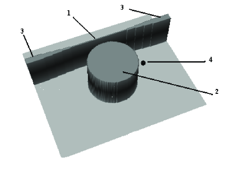
Figure 1: The structure under consideration. The evanescent wave from the slab waveguide (1) is coupled into the disk (2) and back through a small gap between them. The adiabatic waveguide tapers (3) serve for coupling light from optical fibers (not shown) into and out of the waveguide. Cold atoms (4) can be positioned on the disk side.

The disk itself supports a large range of resonant modes. Here, we are mainly interested in the low-loss modes traveling along the disk edge in the form of whispering gallery modes (WGM). While most of the mode energy is confined within the disk, a small part of the mode exists outside the disk as an evanescent field, and it is here that an atom can interact with the light. This atom-light coupling changes the optical properties of the disk mode, which subsequently changes the intensity and/or phase of the light at the output of the linear waveguide. These changes can then be measured to infer the presence of the atom.

In the horizontal direction the linear waveguide and the disk are bordered by air or vacuum with refractive index $n_{cl}=1$. In our calculations we assumed structures made of fused silica with $n_{c}=1.454$ at a wavelength of 780nm. In the vertical direction the structure may be more complicated with several layers in order to give good mode confinement.

A number of numerical and analytical tools have been utilized to investigate the optical properties of such systems, for example coupled mode theory (CMT) hammer ; love , scattering matrix theory rahachou , finite element yamamoto , and finite difference time domain (FDTD) methods hagness . In this work we will use FDTD simulations which provide rigorous numerical results but which are rather time-consuming and therefore not adapt to scan large parameter ranges. We will thus resort to a semi-analytical CMT as a fast tool for a detailed design parameter analysis. These two methods complement one another and give a powerful tool for the investigation of micro resonators. In particular, we are interested in the system characteristics dependent on disk diameter, waveguide width, gap width between the linear waveguide and the disk resonator, and the surface quality of the disk.

III Optical properties of waveguide-coupled whispering gallery modes

III.1 Finite difference time domain calculations

The first method we use to investigate the resonance behavior of the microdisk is by FDTD simulations. Here, Maxwell’s equations are discretized in space and time, and the time evolution of the electromagnetic fields is numerically calculated on this grid. To obtain high accuracy it is necessary to make the cells much smaller than the optical wavelength, which leads to long calculation times, in particular for a three-dimensional (3D) model.

In two dimensions it is possible to perform direct FDTD simulations for relatively large disks of diameter $>50\mu$m. In 3D, simulations are only feasible for small disk diameters. However, comparisons of 2D and 3D simulations for small disk diameters have shown reasonable agreement. In the rest of this paper, we will thus restrict ourselves to simplified 2D calculations, where the disk and waveguide modes are calculated for a geometry infinitely extended in the vertical ($y$) direction. The 3D modes are assumed to be simple slices of thickness $d_{y}$ of these infinite modes. For the calculations presented in this work we always assume $d_{y}=5\mu$m. We will also limit the calculations to electric fields polarized along the $y$ direction, i.e., to TE modes only.

In this case, Maxwell’s equations for the electric and magnetic fields, $E_{y}$, $H_{x}$, and $H_{z}$ reduce to

$$\frac{\partial{H}_{x}}{\partial{t}} = -\frac{1}{\mu}_{0}\frac{\partial{E}_{y}}{\partial{z}},$$ (1)

$$\frac{\partial{H}_{z}}{\partial{t}} = -\frac{1}{\mu}_{0}\frac{\partial{E}_{y}}{\partial{x}},$$ (2)

$$\frac{\partial{E}_{y}}{\partial{t}} = -\frac{1}{\varepsilon}(\frac{\partial{H}_{z}}{\partial{x}}-\frac{\partial{H}_{x}}{\partial{z}}),$$ (3)

where $\mu_{0}$ and $\varepsilon$ are the magnetic and electric permeability, respectively. The FDTD simulations solve Eqs. (1)-(3) on a spatial grid for a given initial field distribution. We used the so-called unsplit perfectly matched layer (UPLM) boundary conditions berenger and a uniform discretization with a step size range of 0.02$\mu$m to 0.08$\mu$m in the $x$ and $z$ directions and with a time step range of $4.45\times{10}^{-17}$s to $1.78\times{10}^{-16}$s.

For our calculations the initial condition was such that the disk was empty and that light was pumped into the lowest transverse mode of the linear waveguide from one end. The incoming light was either a continuous wave or a 30fs Gaussian pulse. In the former case, we are interested in the steady state field distribution which, for example, allows us to observe the resonant disk mode and the evanescent field. Pulsed input allows the calculation of the output power at the other end of the linear waveguide as a function of frequency, i.e., the transmission spectrum, by applying a discrete Fourier transform on the output field, calculating the Poynting power density and integrating over the waveguide cross-section.

III.2 Coupled mode theory

We complement the numerical FDTD results with a semi-analytical CMT. For this, it is assumed that the linear waveguide supports only a single transverse mode, while the disk supports two degenerate, counter-propagating WGM. The pumped waveguide mode only couples to the forward propagating disk mode, but scattering due to side-wall roughness may couple light into the second mode. Both WGM are coupled to the waveguide mode via their evanescent fields at point 1 in Fig. 1. For the calculations we closely follow the work by Rowland and Love love .

First, the WGM are obtained as solutions of Eqs. (1)-(3) in cylindrical coordinates. This gives mode functions of the form

$$E_{WGM}(r,\phi)=\left\{\begin{array}[]{ll}\frac{J_{l}(kn_{c}r)}{J_{l}(kn_{c}R)}e^{\pm il\phi}&\quad\mbox{ for }r<R\\ \frac{H_{l}^{(1)}(kn_{cl}r)}{H_{l}^{(1)}(kn_{cl}R)}e^{\pm il\phi}&\quad\mbox{ for }r>R\end{array}\right.$$ (4)

where $J_{l}$ are Bessel functions and $H_{l}^{(1)}$ are Hankel functions of the first kind, and $R$ is the disk radius. The eigenvalue equation for these modes is given by

$$n_{c}\frac{{J}_{l+1}(kn_{c}R)}{{J}_{l}(kn_{c}R)}=n_{cl}\frac{H^{(1)}_{l+1}(kn_{cl}R)}{H^{(1)}_{l}(kn_{cl}R)}.$$ (5)

As all WGM are lossy, the eigenvalues are complex

$$k=k_{r}-ik_{i}$$ (6)

and the intrinsic quality factor of the WGM is given by love

$$Q_{WGM}=\frac{k_{r}}{2k_{i}}.$$ (7)

Similarly, the mode functions $E_{lin}$ of the linear waveguide are calculated for the same wavenumber $k$.

The second step of the CMT is to write the total light field as a superposition of disk and waveguide mode

$$E(x,z)=a_{1}(z){E}_{lin}(x,z)+a_{2}(z){E}_{WGM}(x,z).$$ (8)

The coupled mode equations read

$$\frac{da_{1}}{dz} = -i{\beta}_{lin}a_{1}+i{C}(z)a_{2},$$ (9)

$$\frac{da_{2}}{dz} = -i{\beta}_{WGM}(z)a_{2}+i{C}(z)a_{1},$$ (10)

where $\beta_{lin}$ and $\beta_{WGM}$ are the propagation constants of the waveguide and the WGM, respectively, and $C(z)$ is the position-dependent coupling coefficient obtained by calculating the mode overlap of waveguide and disk. For details of this calculations see Ref. love .

Finally, integrating Eqs. (9) and (10) over $z$ in the region of significant coupling around point 1 in Fig. 1 yields the coupler transmission matrix $T$ which relates the waveguide and disk output fields to the inputs,

$$\left(\begin{array}[]{c}a_{1}\\ a_{2}\end{array}\right)_{out}=T\left(\begin{array}[]{c}a_{1}\\ a_{2}\end{array}\right)_{in}$$ (11)

where

$$T=\left(\begin{array}[]{cc}t_{11}&t_{12}\\ t_{21}&t_{22}\end{array}\right).$$ (12)

The cavity decay rate (half width at half maximum) $\kappa_{T}$ of the WGM due to the coupling to the waveguide is

$$\kappa_{T}=|t_{12}|^{2}/(2T_{r})$$ (13)

where $T_{r}=2\pi l/(ck)$ is the round trip time. The corresponding quality factor is

$$Q_{coup}=ck/(2\kappa_{T})=2\pi l/|t_{12}|^{2}.$$ (14)

III.3 System losses

Apart from the intrinsic WGM losses (7) and the coupling losses into the waveguide (14) at least two other loss mechanisms have to be taken into account, intrinsic material losses and surface scattering losses.

The main material loss mechanisms are bulk Rayleigh scattering and ultraviolet and infrared absorption. The corresponding quality factor ${Q}_{mat}$ can be expressed in the form gorodetsky ; vernooy

$${Q}_{mat}=\frac{2n_{c}\pi}{\alpha\lambda},$$ (15)

where $\alpha$ is the loss coefficient and $\lambda=2\pi/k$ is the vacuum wavelength. Material losses for fused silica in the wavelength range near 780nm are of the order of 5dB/km, which gives rise to $Q_{mat}\sim 10^{10}$.

Greater uncertainty is associated with losses due to surface scattering and absorption due to surface roughness or the presence of an absorbing impurity on the surface of the disk. For a given size of surface inhomogeneities (roughness) and correlation length, the surface scattering quality factor ${Q}_{surf}$ has to take into account not only the direct scattering of light out of the disk (”leakage”) but also scattering into other modes with high rates of leakage. Various expressions have been used to describe quality limits due to surface scattering gorodetsky ; vernooy ; banna . In this work, we apply the expression based on the model of Rayleigh scattering by molecule-sized surface clusters gorodetsky

$${Q}_{surf}=\frac{D\lambda^{2}}{2L_{c}\pi^{2}\sigma^{2}},$$ (16)

where $D$ is the disk diameter, $\sigma$ is the root-mean-square of the surface roughness and $L_{c}$ the surface correlation length. As was reported in lee , the numerical values for $\sigma$ and $L_{c}$ can be less than 1nm and 5nm, respectively. In our calculations we used $\sigma$=1nm, $L_{c}$=5nm and $\sigma$=2nm, $L_{c}$=10nm.

The overall cavity quality factor taking all the loss mechanisms discussed above into account is then given by

$$Q^{-1}=Q_{coup}^{-1}+Q_{WGM}^{-1}+Q_{mat}^{-1}+Q_{surf}^{-1}.$$ (17)

This is related to the cavity line width (HWHM) $\kappa$ by

$$Q=ck/(2\kappa)$$ (18)

and to the cavity finesse $F$ by

$$F=Q\frac{\mathrm{FSR}}{ck}\approx Q/l$$ (19)

where $\mathrm{FSR}\approx ck/l$ denotes the free spectral range ($l$ is the mode index of the WGM). For later use we also introduce $\kappa_{loss}=\kappa-\kappa_{T}$ which is the cavity loss rate due to losses into all channels apart from the linear waveguide.

III.4 Results

After describing the building blocks of our calculation, let us now discuss some numerical results for the optical properties of our system. This will serve two purposes: first, to compare our different calculation methods with each other and with available experimental data in order to show the accuracy of our results; second, we need to apply our calculation to the experimental parameters that are of interest in our case, in order to establish a base for the atom-light interaction that will be discussed in the following sections.

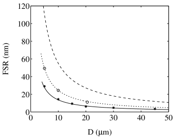
Figure 2: Free spectral range versus disk diameter. The lines present results of analytical calculations at wavelengths 780nm (solid line) and 1550nm (dashed) in fused silica and at 1550nm for $n_{c}=3.2$ (dotted). Corresponding FDTD results are indicated by ($*$), and experimental data hagness by ($\circ$).

We have compared the spatial profile of the WGM obtained from FDTD simulation with the one resulting from a CMT calculation, and found good agreement. We have also looked at the resonance spectrum of the disk for different parameters, and extracted values for the free spectral range (FSR) and the quality factor $Q$. As presented below, here too the agreement was good.

In Fig. 2, we plot the FSR for disk diameters $D$ in the range of 5 - 50$\mu$m, refractive index values 1.454 - 3.2 and wavelengths near 0.78$\mu$m and 1.55$\mu$m. The latter is chosen to compare with previously published results hagness . FDTD simulations and analytically calculated WGM are in excellent agreement with each other and with the experimental data. As expected, the FSR is approximately inversely proportional to the disk diameter.

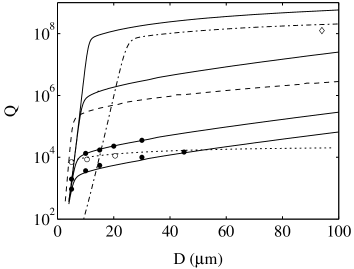
Figure 3: Quality factor $Q$ versus disk diameter for various gap sizes and materials. Solid curves (from bottom to top): CMT results for gap sizes $0.1\mu$m, $0.2\mu$m, $0.5\mu$m, and for the uncoupled disk for $\lambda=780$nm, $n_{c}=1.454$, $\sigma=1$nm, $L_{c}=5$nm, ($\bullet$) represent FDTD simulations. Dashed curve: $n_{c}=2.17$, gap size $0.2\mu$m. CMT results for $\lambda=1550$nm, $\sigma=2$nm, $L_{c}=10$nm: uncoupled disk with $n_{c}=1.444$ (dash-dotted curve), $n_{c}=3.2$ and gap size $0.1\mu$m (dotted curve). Corresponding experimental data is given by ($\diamond$) Kippenberg and ($\circ$) hagness , respectively.

Figure 3 shows the total cavity quality factor $Q$, Eq. (17), dependent on the outer diameter $D$ of the disk and the size of the air gap between disk and linear waveguide. $Q$ was calculated using FDTD and CMT models, which again show excellent agreement. We note that very high quality factors up to about $10^{8}$ can be achieved with the current system for disk diameters of several tens of microns. The upper limit for $Q$ shown in Fig. 3 is the value obtained for a very large air gap, where coupling losses $\kappa_{T}$ are negligible and the cavity quality is limited by the intrinsic and material quality factors $Q_{WGM}$, $Q_{mat}$, and $Q_{surf}$.

Figure 3 also shows data for two different wavelengths and varying refractive index. Note that $Q$ generally increases with increasing refractive index due to the better confinement and therefore weaker coupling to the waveguide. Similarly, $Q$ decreases with increasing wavelength due to stronger waveguide coupling. Nevertheless, for each case there are unique material losses and fabrication uncertainties which may change this general behavior.

To calculate the $Q$ factor for different disk sizes, the index $l$ of the WGM must be changed accordingly to keep the resonant wavelength near 780nm relevant for Rb atoms. The necessary wavelength for optimal mode resonance can be achieved by choosing a precise disk size. We will discuss tuning of the micro resonator later in Sec. VI. Note also that, while the intrinsic quality factor $Q_{WGM}$ is always lower for higher radial modes, the overall $Q$ can in fact be higher due to weaker coupling (smaller losses) to the linear waveguide, which is the dominating loss mechanism for most parameter regimes we are interested in. Table 1 shows the optical properties of a few selected disk-waveguide geometries.

$D$ ($\mu$m)	$l$	$q$	$\lambda$ (nm)	$Q_{1}$	$Q_{2}$	$g_{0}$ (MHz)
30	167	1	778.73	$1.55\times 10^{5}$	$8.44\times 10^{6}$	102.6
30	166	1	783.27	$1.47\times 10^{5}$	$8.05\times 10^{6}$	103.2
30	159	2	780.04	$1.83\times 10^{5}$	$8.85\times 10^{6}$	102.8
15	81	1	780.41	$7.66\times 10^{4}$	$3.82\times 10^{6}$	205.7
45	253	1	780.15	$2.66\times 10^{5}$	$1.40\times 10^{7}$	68.5

Table 1: Optical properties of selected WGM. $Q_{1}$ ($Q_{2}$) is the quality factor $Q$ for a gap size of 0.3$\mu$m (0.6$\mu$m), $l$ and $q$ are the longitudinal and radial mode index, respectively, $g_{0}$ is the single-photon Rabi frequency for an atom at the disk boundary. Surface parameters are $\sigma=2$nm, $L_{c}=10$nm. Results are obtained using CMT.

IV The Jaynes-Cummings model

In this section we introduce a model for the coupling of a two-level atom to the light field outside of the microdisk. We consider two coherent modes with complex amplitudes $\alpha_{+}$ and $\alpha_{-}$ traveling in opposing directions, and assume atom-light coupling to these modes via the respective single-photon Rabi frequencies $g_{+}$ and $g_{-}$. The coupling of the two modes due to imperfections in the disk is accounted for by the introduction of the complex coefficient $\epsilon$, and the model includes the possibility of pumping from either direction with rates $\eta_{+}$ and $\eta_{-}$, where $\eta_{\pm}=t_{21}A_{in,\pm}/\sqrt{T_{r}}$. Here $A_{in,\pm}$ is the amplitude of the pump field in each direction within the waveguide such that $|A_{in,\pm}|^{2}$ is the photon flux in units of photons per second, and $t_{21}$ and $T_{r}$ have been defined in Sec. III.2.

Ignoring the external motion of the atom, the Hamiltonian of this system can be written as $(\hbar=1)$

$$H = -\Delta_{a}\sigma_{11}-\Delta_{c}(a_{+}^{\dagger}a_{-}+a_{-}^{\dagger}a_{-})$$ (20)

$$-i(g_{+}a_{+}^{\dagger}\sigma_{01}-g_{+}^{*}\sigma_{10}a_{+})-i\eta_{+}(a_{+}-a_{+}^{\dagger})$$

$$-i(g_{-}a_{-}^{\dagger}\sigma_{01}-g_{-}^{*}\sigma_{10}a_{-})-i\eta_{-}(a_{-}-a_{-}^{\dagger})$$

$$-i(\epsilon a_{+}^{\dagger}a_{-}-\epsilon^{*}a_{-}^{\dagger}a_{+})\>,$$

where $\Delta_{a}$ and $\Delta_{c}$ are the atomic and resonator detunings, respectively, $\sigma_{10}$ and $\sigma_{01}$ the atomic raising and lowering operators, and $a_{\pm}^{\dagger}$ and $a_{\pm}$ the mode creation and annihilation operators. Here the energy of the lower atomic state has been set to zero. The equation of motion for the density operator of the system can be written as

$$\frac{d}{dt}\rho=-i[H,\rho]+L\rho$$ (21)

where $L$ is the usual linear operator describing cavity and atomic decay with rates $\kappa$ and $\Gamma$ respectively.

Assuming a factorized density operator $\rho$, we find the equations of motion for the elements of the atomic density operator

$$\frac{d}{dt}\rho_{10} = (-\Gamma+i\Delta_{a})\rho_{10}$$ (22)

$$+(g_{+}^{*}\alpha_{+}+g_{-}^{*}\alpha_{-})(\rho_{00}-\rho_{11}),$$

$$\frac{d}{dt}\rho_{11} = -2\Gamma\rho_{11}+(g_{+}^{*}\alpha_{+}+g_{-}^{*}\alpha_{-})\rho_{01}$$ (23)

$$+(g_{+}\alpha_{+}^{*}+g_{-}\alpha_{-}^{*})\rho_{10},$$

and the coherent state amplitudes $\alpha_{\pm}$ obey the equations of motion

$$\frac{d}{dt}\alpha_{+} = (i\Delta_{c}-\kappa)\alpha_{+}-g_{+}\rho_{10}+\eta_{+}-\epsilon\alpha_{-},$$ (24)

$$\frac{d}{dt}\alpha_{-} = (i\Delta_{c}-\kappa)\alpha_{-}-g_{-}\rho_{10}+\eta_{-}+\epsilon^{*}\alpha_{+}.$$ (25)

In this work we are only interested in the stationary solution of these equations of motion. To this end, we first solve the linear set of equations (24) and (25) with respect to $\alpha_{\pm}$. The resulting expressions for $\alpha_{\pm}$ are linear in $\rho_{10}$ and can be inserted into (22). From this and using $\rho_{11}+\rho_{00}=1$, we obtain $\rho_{10}$ as a function of $\rho_{11}$. That and the corresponding results for $\alpha_{\pm}$ can be inserted into (23) to give a real-valued nonlinear equation in $\rho_{11}$ which can be solved by standard numerical techniques. The output field of the linear waveguide is the superposition of the input field transmitted through the waveguide-disk coupler and the light coupled out of the disk,

$$A_{out,\pm}=t_{11}A_{in,\pm}+\frac{t_{12}}{\sqrt{T_{r}}}\alpha_{\pm}.$$ (26)

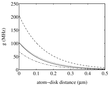
Figure 4: Rabi frequency versus atom-disk distance. Solid curve: $D=30\mu$m, mode indices $(l,q)=(167,1)$; dotted: $D=30\mu$m, $(l,q)=(159,2)$; dashed: $D=15\mu$m, $(l,q)=(81,1)$; dash-dotted: $D=45\mu$m, $(l,q)=(253,1)$.

The Rabi frequency $g_{\pm}$ is given by

$$g_{\pm}=E_{WGM}(\mathbf{x}_{a})\left[\frac{3\Gamma c^{3}}{\omega^{2}d_{y}\int rn(r)^{2}|E_{WGM}(r)|^{2}dr}\right]^{1/2}$$ (27)

where $n(r)=n_{c}$ ($n_{cl}$) for $r<R$ ($r>R$), $d_{y}$ is the disk height, $\omega$ is the atomic transition frequency, and $\mathbf{x}_{a}=(r_{a},\phi_{a})$ is the atomic position in the evanescent field of the disk modes. Figure 4 shows the Rabi frequency depending on the distance of the atom from the disk surface for several disk diameters and mode numbers. The maximum values for $g_{\pm}$ at the disk surface for several selected modes are also given in Table 1.

We note that for efficient atom-mode coupling the atom should be placed within 50-100nm from the disk. Such close proximity should be feasible without the atom being absorbed by the surface, as the van der Waals forces may be counter balanced by blue detuning of the resonator light kimble . In addition, such position resolution is allowed by the 10nm and better ground state sizes achievable in magnetic traps on the atom chip folman . Future work will include exact simulations of the near surface potential.

V Single-atom detection

In the following we will investigate the properties of a microdisk, modeled as a high finesse ring resonator as described in the previous section, as a single-atom detector for quantum information processing on an atom chip. The scheme we discuss here is based on homodyne detection of the phase change of the light at the output of the linear waveguide in the forward direction. There are several advantages of this scheme over a corresponding absorption detection. (i) It allows one to drive the atom far off resonance, in which case the precise tuning of the disk resonator with respect to the atomic transition frequency is of minor importance. Cavity tuning will be discussed in more detail in Sec. VI. (ii) If the additional loss mechanisms discussed in Sec. III.3 are small compared to the disk-waveguide coupling strength, all of the pump light will leave the system through the forward waveguide output. Therefore for most parameter regimes a strong signal can be expected, which allows the use of standard photodetectors rather than sophisticated single-photon counters. (iii) The strong output signal also provides stability of the detection scheme against weak background scattering processes.

Our detection scheme works as follows. The output field of the straight waveguide is mixed with a strong local oscillator field at a 50-50 beamsplitter and the light intensities in the two beamsplitter outputs are measured and integrated over the observation time $\tau$ to give the total number of detected photons $N_{1}$ and $N_{2}$. The signal we are interested in is given by the difference $|N_{1}-N_{2}|$. The phase of the local oscillator is adjusted such that this difference is zero when no atom is interacting with the disk field. The presence of an atom is then inferred from a change in this intensity difference. Assuming that the detection is shot-noise limited, the signal-to-noise ratio $S$ of the atom detection is given by

$$S=\frac{|N_{1}-N_{2}|}{\sqrt{N_{1}+N_{2}}}\approx 2\sqrt{\tau}|A_{out,0}||\sin(\phi-\phi_{0})|$$ (28)

where $\phi$ ($\phi_{0}$) is the phase of the waveguide output field $A_{out,+}$ with (without) an atom, $A_{out,0}$ is the field amplitude without an atom, and we have assumed that only the phase and not the amplitude of the output is changed due to the atom.

The second quantity of interest is the number of photons $M$ spontaneously scattered by the atom during the interaction time, given by

$$M=2\Gamma\tau\rho_{11}.$$ (29)

This should be as small as possible in order to minimize the backaction of the detection process onto the atom. Ideally, $M\ll 1$ corresponds to the limit of non-destructive measurements. Finally, we note that $S$ and $M$ scale differently with interaction time $\tau$. For any given parameters, we can thus choose $\tau$ in such a way to yield a certain, fixed signal-to-noise ratio. As an example, we will in the following consider the number $M_{10}$ of spontaneously scattered photons when $\tau$ is rescaled to give $S=10$,

$$M_{10}=100M/S^{2}.$$ (30)

For simplicity we will assume that the cavity is driven on resonance with the disk modes, $\Delta_{c}=0$, thereby minimizing the effect of other, off-resonant modes. The atom is assumed to be far off resonance with respect to the cavity mode, $\Delta_{a}\gg\Gamma$, such that the effect of the atom is mainly to provide a phase shift of the cavity mode. Under these conditions and in the limit of small atomic saturation we can derive analytical approximations for $S$, $M$ and $M_{10}$ horak

$$S = 4\sqrt{\tau}|A_{in}|\frac{\kappa_{T}g^{2}}{\Delta_{a}\kappa^{2}},$$ (31)

$$M = 4\tau|A_{in}|^{2}\frac{\kappa_{T}g^{2}\Gamma}{\Delta_{a}^{2}\kappa^{2}},$$ (32)

$$M_{10} = 25\frac{\kappa^{2}\Gamma}{\kappa_{T}g^{2}}.$$ (33)

Note that $M_{10}$ is independent of the pump power and of the atomic detuning.

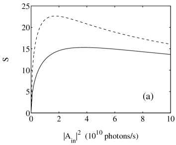
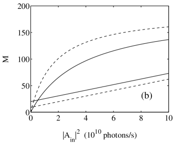
Figure 5: (a) Signal-to-noise ratio versus pump intensity for disk diameter 30$\mu$m (solid line) and 15$\mu$m (dashed). (b) Corresponding photon scattering $M$ (top curves) and $M_{10}$ (bottom). Gap size is 0.3$\mu$m, waveguide width is 0.6$\mu$m, $\sigma=2$nm, $L_{c}=10$nm, $\Delta_{a}=100\Gamma$, $\tau=10\mu$s, and the atom is assumed to sit 50nm away from the disk surface.

In Fig. 5 we show $S$, $M$ and $M_{10}$ as a function of the input power to the linear waveguide. For a weak pump the signal-to-noise ratio increases with power since more photons are coupled into the cavity and interact with the atom. However, because of saturation the atom can only interact with a maximum number of photons in a given interaction time. Hence, $S$ reaches a maximum value, and for stronger pump powers $S$ is decreasing again. The number of spontaneously scattered photons $M$ increases with pump power and finally saturates at the value $\Gamma\tau$. $M_{10}$ shows an approximately linear increase with pump power, indicating that the least perturbing atom detection for a given value of $S$ is achieved for low atomic saturation. There is, however, a trade-off as the required interaction time increases in this limit. For low saturation, $\rho_{11}\ll 1$, the numerical results are accurately described by the approximations (31)-(33).

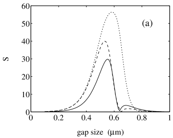
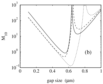
Figure 6: (a) Signal-to-noise ratio $S$ and (b) scattered photons $M_{10}$ versus gap size for weak pumping ($|A_{in}|^{2}=10^{8}$ photons/s). Solid curve: $D=30\mu$m, dashed: $D=15\mu$m for $\sigma=2$nm, $L_{c}=10$nm. Dotted curve: $D=15\mu$m, $\sigma=1$nm, $L_{c}=5$nm. Waveguide width is 0.6$\mu$m, distance atom-disk is 50nm, interaction time is $10\mu$s.

Figure 6 shows $S$ and $M_{10}$ as a function of the gap between the microdisk and the waveguide in the limit of weak atomic saturation ($\rho_{11}<0.03$ for the shown parameter range). For small enough gap sizes, increasing the gap reduces the coupling between disk and waveguide modes and therefore the cavity finesse increases. This leads to improved signal-to-noise ratios and less spontaneous photon scattering by the atom. For very large gaps, on the other hand, the cavity finesse is limited by the additional losses, see Sec. III.3. In this case, increasing the gap even further reduces the number of photons coupled back from the cavity into the waveguide and thus reduces the detected signal. If the cavity-waveguide coupling exactly equals the additional losses, no light is transmitted through the waveguide at all, which leads to the points of $S=0$ and the corresponding divergence of $M_{10}$ observed in the figure. We find numerically that $S$ is maximum and $M_{10}$ is minimum if losses from the disk into the waveguide are about 4-5 times higher than the additional losses.

For the parameters of Fig. 6 we find that the minimum value of $M_{10}$ is 0.85 for a disk diameter of $D=30\mu$m (solid line) and 0.49 for $D=15\mu$m (dashed line). The reason for this difference is mainly that for the smaller disk more energy of the resonant mode is in the evanescent field. This leads to improved coupling of the atom to the mode, that is, to a larger Rabi frequency $g$ as already seen in Fig. 4. For both disk diameters, however, the minimum value of $M_{10}$ is below unity, which indicates that single atoms can be detected while on average scattering less than one photon spontaneously. Moreover, we observe that this minimum value of $M_{10}$ is limited by the additional losses due to surface roughness. If the surface parameters are decreased by a factor of two to $\sigma=1$nm and $L_{c}=5$nm, $M_{10}$ can be as small as 0.13, shown by the dotted curve in Fig. 6(b). In this case, our atom detection scheme approaches the limit of a non-destructive measurement.

Note also that the parameters where optimum single-atom detection is observed correspond to the strong coupling regime of cavity QED QED , defined by $g^{2}/(\kappa\Gamma)\gg 1$. In particular, at the minimum points of $M_{10}$ in Fig. 6 we find $g^{2}/(\kappa\Gamma)=48$ ($D=30\mu$m), 73 ($D=15\mu$m, $\sigma=2$nm, $L_{c}=10$nm), and 290 ($D=15\mu$m, $\sigma=1$nm, $L_{c}=5$nm).

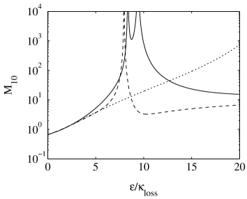
Figure 7: $M_{10}$ versus mode coupling parameter $\epsilon/\kappa_{loss}$ for $D=15\mu$m, gap size $0.5\mu$m, $\sigma=2$nm, $L_{c}=10$nm, $\Delta_{a}=100\Gamma$, $|A_{in}|^{2}=10^{8}$ photons/s. Solid curve: $\Delta_{c}=0$, dashed: $\Delta_{c}=\epsilon$, dotted: $\Delta_{c}=-\epsilon$.

Finally, in Fig. 7 we show the effect of mode coupling between the two counter-propagating WGM on the single-atom detection. For $\epsilon$ smaller than the total cavity linewidth $\kappa$, the main effect of mode coupling is to increase the loss rate of the forward propagating mode. This decreases the mode quality factor and therefore increases $M_{10}$. For $\epsilon>\kappa$, the strong coupling lifts the degeneracy between the counter-propagating modes. The resulting new frequency eigenmodes of the disk are shifted in frequency by $\pm\epsilon$ with respect to the uncoupled modes. Tuning one of these coupled modes into resonance with the pump may thus seem advantageous. However, as can be seen from the corresponding curves in Fig. 7, this is not the case for some parameter regions. Several effects play a role here: (i) our detection scheme only measures the forward propagating output of the linear waveguide and thus is sensitive to the phase difference between the two coupled modes, which in turn changes with the frequency shift; (ii) coupling to the backward propagating mode can be regarded as an additional loss, which shifts the position of the divergences of $M_{10}$ already observed in Fig. 6; (iii) strong coupling between the counter-propagating modes fixes their relative phase, which creates a standing-wave pattern at the disk surface. Thus, the atom detection becomes dependent on the position of the atom. In particular, if the atom is trapped at a node of the standing wave, no interaction with the light occurs and atom detection is impossible. The interplay between these effects explains the features of Fig. 7. Note finally that for high quality disk resonators only weak mode coupling is expected, for example, in Ref. Kippenberg a mode coupling parameter $\epsilon/\kappa_{loss}$ of 1.5 has been reported.

VI Experimental considerations and tunability

In this section we consider the feasibility of a microdisk resonator in a realistic experiment on an atom chip. In particular we discuss the effects of finite fabrication tolerances, of temperature fluctuations, and various possibilities to tune the resonance frequencies of the disk.

Let us first consider fabrication imperfections due to edge roughness, which changes the disk diameter, or due to impurities, which change the index of refraction. To first order, these uncertainties affect the mode resonance through the simple relation klitzing

$$\Delta\nu/\nu=-\Delta n/n-\Delta D/D,$$ (34)

where $\Delta\nu$, $\Delta n$, and $\Delta D$ are the changes of the resonance frequency, the refractive index, and the disk diameter, respectively. Assuming typical fabrication tolerances for the disk diameter of a few nm and for the refractive index of the order of $10^{-5}$ therefore leads to frequency shifts of the order of tens of GHz.

Similarly, temperature fluctuations typically give rise to changes of the refractive index of the order of $10^{-6}$ per $1^{0}$C. This again will shift resonance frequencies of the microdisk by amounts in the GHz regime. Therefore, methods to dynamically tune the disk resonator have to be implemented on the chip in order to provide frequency stability.

Tunable photonics is also needed if we want to trap, manipulate, and measure different kinds of atoms or atoms in various internal states. Accurate control of the light-matter interaction is especially critical if one is to enable the exploitation of quantum technology, for example, in the case of quantum communication in order to convert a flying quantum bit (qubit) in the form of a photon into a storage qubit (atom), in the case of quantum computing where single qubit rotations, e.g., between two hyperfine states, are needed, or in the case of sensors to measure interference patterns.

As already noted, high $Q$ devices such as microspheres, Fabry-Perot cavities, or microdisks are an extremely effective tool for the delicate manipulation and measurement of subtle quantum states, where a single photon can interact many times with the same atom so that significant interaction can be achieved. However, such strong coupling requires that the device is kept on resonance with the exact frequency close to the chosen atom transition horak ; klitzing .

In general, the FSR of a microdisk is orders of magnitude larger than the linewidth, and therefore coincidences between the fundamental transverse WGM and specific atomic transitions are extremely unlikely. To keep a WGM resonance near the wavelength of interest we thus need to change the diameter or the refractive index of the disk. In order to achieve any given frequency, the tuning range has to be of the order of the FSR. Furthermore, the procedure should be stable, reversible, and fast enough to compensate for temporal instabilities such as those arising from temperature fluctuations of the chip. Under these conditions a resonant mode close to the required atomic frequency can always be found, even if the disk was initially fabricated with some mismatch in diameter or in refractive index.

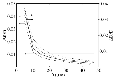
Figure 8: Required change of disk diameter and refractive index for a full FSR scan versus disk diameter at $\lambda=780$nm. $\Delta D/D$ and $\Delta n/n$ are presented by dotted and dash-dotted curves for $n=1.454$, and by solid and dashed curves for $n=2.17$, respectively. Typical values for actual materials are also presented by the long base arrows.

In order to scan a full FSR we require that $\Delta\nu/\nu\approx 1/l$, where $l$ is the longitudinal mode index. Together with Eq. (34) this yields the required relative change of disk diameter and refractive index. Results for this relative change are shown in Fig. 8 versus the disk diameter for fused silica ($n=1.454$ at $\lambda=780$nm) and for $n=2.17$ at $\lambda=780$nm. Note however that since a few higher order radial modes can also be used for some applications, there may in fact exist several usable resonances within each FSR.

At least three possibilities may be considered to realize a tunable microdisk resonator: UV, electro-optical, and piezo tuning.

UV tuning was reported in javris . There, it has been shown that it is possible to change the refractive index of Ge doped silica by up to $\Delta n=0.006$ using UV radiation. The drawback is that this procedure is not reversible.

In the case of electro-optical tuning, the effect is achieved by a uniform electric field that changes the refractive index and thus allows one to tune the resonance wavelength. The idea is to cover both the bottom and the top of the disk with a metal layer, and apply a voltage to create the necessary electric field. For example, electro-optic crystaline materials usually have a relative change of refractive index of $0.01\%-1\%$ for a field of $10^{6}$V/m (5V for our $5\mu$m disk thickness). Though demanding a more complex fabrication process, such crystals may indeed be used. Figure 8 shows that disk diameters as small as $15\mu$m will enable a full FSR scan assuming $\Delta n/n=1\%$. Other methods for such changes of the refractive index also exist. For example, it was reported in djordjev that tuning an InP microdisk can be achieved utilizing free carrier injection, which results in $\Delta n\sim 0.002$ up to $\Delta n\sim 0.01$.

By using a piezo effect one can change the diameter of the disk. In this case, one has to fabricate the disk from a transparent piezo material. The voltage necessary for tuning will be obtained as above by two electrodes evaporated below and above the device. Transparent piezo materials (such as BaTiO₃) have a piezo electric coefficient of order $10^{-10}$m/V which leads to $\Delta D/D=0.003$ for electric fields of $30\times 10^{6}$V/m (150V for our $5\mu$m disk thickness). Figure 8 shows that in this case disk diameters as small as $30\mu m$ will enable a full FSR scan. For both disk size tuning and refractive index tuning, higher voltages and more exotic materials should allow for even smaller disk sizes.

VII Summary and conclusions

We have investigated the feasibility of initiating strong interaction between photons and single atoms on an atom chip by utilizing microdisks as high $Q$ resonators.

Our calculations show that whispering gallery modes with high quality factors of up to $10^{8}$ can be supported by disks with diameters of several tens of microns. Single-atom detection with high signal-to-noise ratios and practically no spontaneous photon scattering can be achieved in such a system, and hence non-destructive measurements may be possible.

We have also discussed different methods which would allow one to tune the resonance frequencies of a microdisk over a full free spectral range.

These results suggest that the regime of strong coupling between atoms and photons can be achieved in optical resonators as small as five microns in diameter. This could open the way for compact arrays for quantum information processing.

- (1) R. E. Slusher, A. F. J. Levi, U. Mohideen, S. L. McCall, S. J. Paerton, and R. A. Logan, Appl. Phys. Lett. 63, 1310 (1993). D. Sadot and E. Boimovich, IEEE Comm. Magazine 36 (12), 50 (1998).
- (2) F. Vollmer, D. Braun, A. Libchaber, M. Khoshsima, I. Teraoka, and S. Arnold, Appl. Phys. Lett. 80, 4057 (2002).
- (3) T. Pellizzari, S. A. Gardiner, J. I. Cirac, and P. Zoller, Phys. Rev. Lett. 75, 3788 (1995); S. J. van Enk, J. I. Cirac, and P. Zoller, Science 279, 205 (1998); C. J. Hood, M. S. Chapman, T. W. Lynn, and H. J. Kimble, Phys. Rev. Lett. 80, 4157 (1998); P. W. H. Pinkse, T. Fisher, P. Maunz, and G. Rempe, Nature 404, 365 (2000).
- (4) M. Pelton, C. Santori, G. S. Solomon, O. Benson, and Y. Yamamoto, Eur. Phys. J. D 18, 179 (2002); P. Michler, A. Kiraz, C. Becher, L. Zhang, E. Hu, A. Imamoglu, W. V. Schoenfeld, and P. Petroff, Phys. Status Solidi B 224, 797 (2001); J. McKeever, J. R. Buck, A. D. Boozer, and H. J. Kimble, arXiv: quant-ph/0403121 (2004).
- (5) The Physics of Quantum Information, edited by D. Bouwmeester, A. Ekert, and A. Zeilinger (Springer-Verlag, Berlin, 2000).
- (6) Proceedings of the International Workshop on Matter Wave Interferometry, edited by G. Badurek, H. Rauch, and A. Zeilinger [Physica (Amsterdam) 151B, No. 1-2 (1988)]; Atom Interferometry, edited by P. Berman, Academic Press (1997); A. Peters, K. Y. Chung, and S. Chu, Nature 400, 849 (1999); T. L. Gustavson, A. Landragin, and M. A. Kasevich, J. Class. Quant. Grav. 17, 2385 (2000) and references there in; For atomchip interferometers, see for example: E. A. Hinds, C. J. Vale, and M. G. Boshier, Phys. Rev. Lett. 86, 1462 (2001); W. Hänsel, J. Reichel, P. Hommelhoff, and T. W. Hänsch, arXiv: quant-ph/0106162 (2001); E. Andersson, T. Calarco, R. Folman, M. Andersson, B. Hessmo and J. Schmiedmayer, Phys. Rev. Lett. 88, 100401 (2002).
- (7) For a review of quantum computing in general see for example, Phys. World 11 (3), 33 (1998), special issue on quantum information, edited by M. B. Plenio and V. Vedral; M. B. Plenio, Contemp. Phys. 39, 431 (1998); A. M. Steane, Rep. Prog. Phys. 61, 117 (1998).
- (8) T. J. Kippenberg, S. M. Spillane, D. K. Armani, and K. J. Vahala, Appl. Phys. Lett. 83, 797 (2003); D.K. Armani, T.J. Kippenberg, S. M. Spillane, and K. J. Vahala, Nature 421, 925 (2003); V. Zwiller, S. Fälth, J. Persson, W. Seifert, L. Samuelson, and G. Björk, J. Appl. Phys. 93, 2307 (2003).
- (9) R. Folman, P. Krueger, J. Schmiedmayer, J. Denschlag, and C. Henkel Adv. At. Mol. Opt. Phys. 48, 263 (2002).
- (10) J. Reichel, Appl. Phys. B 74, 469 (2002).
- (11) P. Horak, B. G. Klappauf, A. Haase, R. Folman, J. Schmiedmayer, P. Domokos, and E. A. Hinds, Phys. Rev. A 67, 043806 (2003).
- (12) B. Lev, K. Srinivasan, P. Barclay, O. Painter, and H. Mabuchi, arXiv: quant-ph/0402093 (2004).
- (13) V. Lefevre-Seguin and S. Haroche, Mater. Sci. Eng. B 48, 53 (1997).
- (14) W. von Klitzing, R. Long, V. S. Ilchenko, J. Hare, and V. Lefevre-Seguin, New J. Phys. 3, 14 (2001).
- (15) D. W. Vernooy, V. S. Ilchenko, H. Mabuchi, E. W. Streed, and H. J. Kimble, Opt. Lett. 23, 247 (1998); D. W. Vernooy, A. Furusawa, N. P. Georgiades, V. S. Ilchenko, and H. J. Kimble, Phys. Rev. A 57, R2293 (1998).
- (16) R. Stoffer, K. R. Hiremath, and M. Hammer, Proceedings of the International School of Quantum Electronics, 39th course, Erice, Sicily (October 2003); M. Hammer, K. R. Hiremath, and R. Stoffer, AIP Conference Proceedings, Melville, New York (to appear in 2004).
- (17) D. R. Rowland and J. D. Love, IEE Proceedings-J 140, 177 (1993).
- (18) A. I. Rahachou and I. V. Zozoulenko, arXiv: physics/0307024 (2003).
- (19) T. Yamamoto and M. Koshiba, J. Lightwave Technol. 11, 400 (1993).
- (20) S. C. Hagness, D. Rafizadeh, S. T. Ho, and A. Taflove, J. Lightwave Technol. 15, 2154 (1997); D. Rafizadeh, J. P. Zhang, S. C. Hagness, A. Taflove, K. A. Stair, S. T. Ho, and R. C. Tiberio, Opt. Lett. 22, 1244 (1997).
- (21) J. P. Berenger, J. Comput. Phys. 114, 185 (1994); S. D. Gedney, IEEE Trans. Antennas Propagation 114, 1630 (1996); C. E. Reuter, R. M. Joseph, E. T. Thiele, D. S. Katz, and A. Taflove, IEEE Microwave Guided Wave Lett. 4, 344 (1994).
- (22) M. L. Gorodetsky, A. A. Savchenkov, and V. S. Ilchenko, Opt. Lett. 21, 453 (1996).
- (23) D. W. Vernooy, V. S. Ilchenko, H. Mabuchi, E. W. Streed, and H. J. Kimble, Opt. Lett. 23, 247 (1998).
- (24) S. Banna, D. Schieber, and L. Schächter, J. Appl. Phys. 95, 4415 (2004); B. E. Little and S. T. Chu, 21, 1390 (1996); A. I. Rahachou and I. V. Zozoulenko, arXiv: physics/0305111 (2003); D. G. Hall, Opt. Lett. 6, 601 (1981); J. J. Barroso, J. P. L. Neto, and K. G. Kostov, IEEE Trans. Plasma Sci. 31, 752 (2003).
- (25) K. K. Lee, D. R. Lim, and L. C. Kimerling, Opt. Lett. 26, 1888 (2001); K. H. Guenter and P. G. Wierer, Proc. SPIE 401, 266 (1983).
- (26) R. A. Javris, J. D. Love, A. Durandet, G. D. Conway, and R. W. Boswell, Electron. Lett. 32, 550 (1996).
- (27) K. Djordjev, S.-J. Choi, S.-J. Choi, and P. D. Dapkus, IEEE Photon. Technol. Lett. 14, 828 (2002).