Loophole-free test of quantum non-locality using high-efficiency homodyne detectors

Abstract

We provide a detailed analysis of the recently proposed setup for a loophole-free test of Bell inequality using conditionally generated non-Gaussian states of light and balanced homodyning. In the proposed scheme, a two-mode squeezed vacuum state is de-gaussified by subtracting a single photon from each mode with the use of an unbalanced beam splitter and a standard low-efficiency single-photon detector. We thoroughly discuss the dependence of the achievable Bell violation on the various relevant experimental parameters such as the detector efficiencies, the electronic noise and the mixedness of the initial Gaussian state. We also consider several alternative schemes involving squeezed states, linear optical elements, conditional photon subtraction and homodyne detection.

I Introduction

In their seminal 1935 paper, Einstein, Podolsky, and Rosen (EPR) advocated that if “local realism” is taken for granted, then quantum theory is an incomplete description of the physical world Einstein35 . The EPR argument gained a renewed attention in 1964, when John Bell derived his famous inequalities, which must be satisfied within the framework of any local realistic theory Bell64 . The violation of Bell inequalities, predicted by quantum mechanics, has since then been observed in many experiments Freedman72 ; Aspect81 ; Aspect82a ; Aspect82b ; Kwiat95 ; Weihs98 ; Rowe01 ; Tittel98 , thereby disproving the concept of local realism. So far, however, all these tests suffered from either a detector-efficiency loophole or a locality loophole Pearle70 ; Kwiat94 , that is, the measured correlations may be explained in terms of local realistic theories exploiting the low detector efficiency or the timelike interval between the two detection events Santos92 ; Gisin99 ; Massar02 .

A test of Bell inequality violation typically involves two distant parties, Alice and Bob, who simultaneously carry out measurements on parts of a shared quantum system that is prepared in an entangled state. Both parties randomly and independently decide between one of two possible quantum measurements $a_{1},a_{2}$ and $b_{1},b_{2}$. To avoid the locality loophole, the measurement events (including the choice of the measurement) at Alice’s and Bob’s sites must be spacelike separated. This suggests that optical systems are particularly suitable candidates for the test of Bell inequality violations. The technology of generation of entangled states of photons is very well mastered today Kwiat95 and the prepared entangled states can be distributed over long distances via low-loss optical fibers Weihs98 . However, the currently available single-photon detectors suffer from a too low efficiency $\eta$, which opens the so-called detector-efficiency loophole. This loophole has been closed in a recent experiment with two trapped ions Rowe01 . However, the ions were held in a single trap, only several micrometers apart, so that the measurement events were not space-like separated. It was suggested that two distant trapped ions can be entangled via entanglement swapping by first preparing an entangled state of an ion and a photon on each side and then projecting the two photons on a maximally entangled singlet state Simon03 ; Feng03 ; Duan03 ; Browne03 . This technique could be used to close the locality loophole in the Bell test with trapped ions Simon03 . Very recently, the first step toward this goal, namely the entanglement between a trapped ion and a photon emitted by the ion, has been observed experimentally Blinov04 . However, the entanglement swapping would require interference of two photons emitted by two different ions, which is experimentally very challenging.

An interesting alternative to the atom-based approaches Simon03 ; Fry95 ; Freyberger96 is represented by all-optical schemes involving balanced homodyne detection, which can exhibit very high detection efficiency Polzik92 ; Grosshans03 . Unfortunately, the entangled two-mode squeezed state that can easily be generated experimentally Ou92 ; Schori02 ; Bowen04 cannot be directly employed to test Bell inequalities with homodyning. This state is described by a positive definite Gaussian Wigner function, which thus provides a local hidden variable model that can explain all correlations established via quadrature measurements carried by balanced homodyne detectors. Similarly as in the case of purification of continuous variable entanglement Eisert02 ; Fiurasek02 ; Giedke02 ; Browne03b ; Eisert04 , one has to go beyond the class of Gaussian states and Gaussian operations. For instance, it is possible to obtain a violation of Bell inequality with Gaussian two-mode squeezed vacuum state by performing photon-counting measurements Banaszek98 or the rather abstract measurements described in Refs. Chen02 ; Mista02 ; Filip02 . However, in contrast to balanced homodyning, these measurements are either experimentally infeasible or suffer from a very low detection efficiency.

In order to close the detection loophole by using homodyne detectors, it is necessary to employ highly non-classical non-Gaussian entangled state whose Wigner function is not positive definite. Several recent theoretical works indeed demonstrated that violation of Bell inequalities can be observed using balanced homodyning Gilchrist98 ; Gilchrist99 ; Munro99 ; Wenger03 , if specific entangled light states such as pair-coherent states, squeezed Schrödinger cat-like states, or specifically tailored finite superpositions of Fock states, are available. However, no feasible experimental scheme is known that could generate the states required in Refs. Gilchrist98 ; Gilchrist99 ; Munro99 ; Wenger03 .

Recently, we have shown that a very simple non-Gaussian state obtained from two-mode squeezed vacuum by subtracting a single photon from each mode Opatrny00 ; Cochrane02 ; Olivares03 can exhibit Bell violation with homodyning Sanchez04 . An essential feature of our proposal is that the photon subtraction can be successfully performed with low-efficiency single-photon detectors, which renders the setup experimentally feasible. In fact, the basic building block of the scheme, namely the de-gaussification of a single-mode squeezed vacuum via single-photon subtraction, has been recently successfully implemented experimentally Wenger04 .

In the present paper, we provide a thorough analysis of the scheme proposed in Ref. Sanchez04 . We present the details of the calculation of the Bell factor for a realistic setup that takes into account mixed input states, losses, added noise and imperfect detectors. Moreover, we shall also discuss several alternative schemes that involve the subtraction of one, two, three, or four photons. The present paper is organized as follows. In Section II, we describe the proposed experimental setup and we introduce the Bell-CHSH inequalities. We then provide a simple pure-state analysis of the scheme assuming ideal detectors, which gives an upper bound on the achievable Bell violation. In Section III, we present the mathematical description of a realistic setup with imperfect detectors, losses and noise. Besides the scheme where a single photon is subtracted on each side, we will also analyze a scheme where two photons are subtracted on each side. This latter scheme yields slightly higher Bell violation but only at the expense of a very low probability of state preparation. Several other schemes composed of squeezed state sources, linear optics, and photon subtraction, are discussed in Section IV. Finally, the conclusions are drawn in Section V.

II Feasible Bell test with homodyne detection

II.1 Proposed optical setup

The conceptual scheme of the proposed experimental setup is depicted in Fig. 1. A source generates a two-mode squeezed vacuum state in modes A and B. This can be accomplished, e.g., by means of non-degenerate parametric amplification in a $\chi^{(2)}$ nonlinear medium or by generating two single-mode squeezed vacuum states and combining them on a balanced beam splitter. Subsequently, the state is de-gaussified by conditionally subtracting a single photon from each beam. A tiny part of each beam is reflected from a beam splitter BS_A (BS_B) with a high transmittance T. The reflected portions of the beams impinge on single-photon detectors such as avalanche photodiodes. A successful photon number subtraction is heralded by a click of each photodetector PD_A and PD_B Olivares03 . In practice, the photodetectors exhibit a single-photon sensitivity but not a single photon resolution, that is, they can distinguish the absence and presence of photons but cannot measure the number of photons in the mode. Nevertheless, this is not a problem here because in the limit of high $T$, the most probable event leading to the click of a photodetector is precisely that a single photon has been reflected from the squeezed beam on the beam splitter. The probability of an event where two or more photons are subtracted from a single mode is smaller by a factor of $\approx 1-T$ and becomes totally negligible in the limit of $T\rightarrow 1$. Another important feature of the scheme is that the detector efficiency $\eta$ can be quite low because small $\eta$ only reduces the success rate of the conditional single-photon subtraction but it does not significantly decrease the fidelity of this operation. These issues will be discussed in detail in Section III.

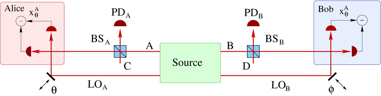
Figure 1: Conceptual scheme of the proposed experimental setup for observing violation of Bell inequalities with balanced homodyning. The source emits two-mode squeezed vacuum mode in modes A and B. A small part of the beams is subtracted on two unbalanced beam splitters BS_A and BS_B and sent on single-photon detectors PD_A and PD_B.

After generation of the non-Gaussian state, the two beams A and B together with the appropriate local oscillators LO_A and LO_B are sent to Alice and Bob, who then randomly and independently measure one of two quadratures $x_{\theta_{j}}^{A}$, $x_{\phi_{k}}^{B}$ characterized by the relative phases $\theta_{1},\theta_{2}$ and $\phi_{1},\phi_{2}$ between the measured beam and the corresponding local oscillator. The rotated quadratures $x_{\theta}^{A}=\cos\theta\,x^{A}+\sin\theta\,p^{A}$ and $x_{\phi}^{B}=\cos\phi\,x^{B}+\sin\phi\,p^{B}$ are defined in terms of the four quadrature components of modes A and B that satisfy the canonical commutation relations $[x^{j},p^{k}]=i\delta_{jk}$, $j,k\in\{A,B\}$.

To avoid the locality loophole, the whole experiment has to be carried out in the pulsed regime and a proper timing is necessary. In particular, the measurement events on Alice’s and Bob’s sides (including the choice of phases) have to be space-like separated. A specific feature of the proposed setup is that the non-Gaussian entangled state needed in the Bell test is generated conditionally when both “event-ready” detectors Bell PD_A and PD_B click. However, we would like to stress that this does not represent any loophole if proper timing is satisfied. Namely, in each experimental run, the detection of the clicks (or no-clicks) of photodetectors PD_A and PD_B at the source should be be space-like separated from Alice’s and Bob’s measurements. This guarantees that the choice of the measurement basis on Alice’s and Bob’s sides cannot in any way influence the conditioning measurement or vice versa Sanchez04 ; Simon03 ; Bell ).

To demonstrate that the experimental data recorded by Alice and Bob are incompatible with the concept of local realism, we shall consider the Bell-CHSH inequality originally devised for two-qubit system CHSH . In this scenario, Alice (Bob) randomly and independently decides between one of two possible quantum measurements $a_{1},a_{2}$ ($b_{1},b_{2}$) which should have only two possible outcomes $+1$ or $-1$. We define the Bell parameter

$$S=\langle a_{1}b_{1}\rangle+\langle a_{1}b_{2}\rangle+\langle a_{2}b_{1}\rangle-\langle a_{2}b_{2}\rangle,$$ (1)

where $\langle a_{j}b_{k}\rangle$ denotes the average over the subset of experimental data where Alice measured $a_{j}$ and, simultaneously, Bob measured $b_{k}$. If the observed correlations can be explained within the framework of the local-hidden variable theories, then $S$ must satisfy the Bell-CHSH inequality $|S|\leq 2$.

In the proposed experiment, Alice and Bob measure quadratures which have continuous spectrum. We discretize the quadratures by postulating that the outcome is $+1$ when $x\geq 0$ and $-1$ otherwise. The two different measurements on each side correspond to the choices of two relative phases $\theta_{1},\theta_{2}$ and $\phi_{1},\phi_{2}$. Quantum mechanically, the correlation $E(\theta_{j},\phi_{k})\equiv\langle a_{j}b_{k}\rangle$ can be expressed as

$$E(\theta_{j},\phi_{k})=\int_{-\infty}^{\infty}\mathrm{sign}(x_{\theta_{j}}^{A}x_{\phi_{k}}^{B})P(x_{\theta_{j}}^{A},x_{\phi_{k}}^{B})dx_{\theta_{j}}^{A}dx_{\phi_{k}}^{B},$$ (2)

where $P(x_{\theta_{j}}^{A},x_{\phi_{k}}^{B})\equiv\langle x_{\theta_{j}}^{A},x_{\phi_{k}}^{B}|\rho_{c,AB}|x_{\theta_{j}}^{A},x_{\phi_{k}}^{B}\rangle$ is the joint probability distribution of the two commuting quadratures $x_{\theta_{j}}^{A}$ and $x_{\phi_{k}}^{B}$, and $\rho_{c,AB}$ denotes the (normalized) conditionally generated non-Gaussian state of modes A and B. In practice, the correlations would be determined from the subset of the experimental data corresponding to the successful conditional de-gaussification, i.e., Alice and Bob would discard all results obtained in measurement runs where either PD_A or PD_B did not click. We emphasize again that this does not open any loophole in the Bell test.

II.2 Ideal photodetectors

We shall first present a simplified description of the setup, assuming ideal photodetectors ($\eta_{\mathrm{PD}}=1$) with single-photon resolution and conditioning on detecting exactly a single photon at each detector Opatrny00 ; Cochrane02 . This idealized treatment is valuable since it provides an upper bound on the practically achievable Bell factor $S$. Moreover, as noted above, in the limit of high transmittance of $BS_{A}$ and $BS_{B}$, $T\rightarrow 1$, the realistic (inefficient) detector with single-photon sensitivity is in our case practically equivalent to these idealized detectors.

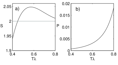
Figure 2: (a) Bell factor $S$ is plotted as a function of the effective squeezing parameter $T\lambda$ for $\theta_{1}=0$, $\theta_{2}=\pi/2$, $\phi_{1}=-\pi/4$ and $\phi_{2}=\pi/4$. (b) Probability $P$ of successful conditional generation of the state $|\psi_{\mathrm{out}}\rangle$ as a function of the effective squeezing parameter $T\lambda$, assuming $T=0.95$.

The two-mode squeezed vacuum state can be expressed in the Fock state basis as follows,

$$|\psi_{\mathrm{in}}(\lambda)\rangle_{AB}=\sqrt{1-\lambda^{2}}\sum_{n=0}^{\infty}\lambda^{n}|n,n\rangle_{AB},$$ (3)

where $\lambda=\tanh(s)$ and $s$ is the squeezing constant. In the case of ideal photodetectors, the photon number subtraction results in the state $|\psi_{\mathrm{out}}\rangle\propto a_{A}a_{B}|\psi_{\mathrm{in}}(T\lambda)\rangle$, where $a_{A,B}$ are annihilation operators and the parameter $\lambda$ is replaced by $T\lambda$ in order to take into account the transmittance of $BS_{A}$ and $BS_{B}$. A detailed calculation yields

$$|\psi_{\mathrm{out}}\rangle_{AB}=\sqrt{\frac{(1-T^{2}\lambda^{2})^{3}}{1+T^{2}\lambda^{2}}}\sum_{n=0}^{\infty}(n+1)(T\lambda)^{n}|n,n\rangle_{AB},$$ (4)

and the probability of the conditional preparation of state (4) can be expressed as

$$\mathcal{P}=(1-T)^{2}\lambda^{2}(1-\lambda^{2})\frac{1+T^{2}\lambda^{2}}{(1-T^{2}\lambda^{2})^{3}}.$$ (5)

For pure states exhibiting perfect photon-number correlations, the correlation coefficient (2) depends only on the sum of the angles, $E(\theta_{j},\phi_{k})=\mathcal{E}(\theta_{j}+\phi_{k})$. With the help of the general formula derived by Munro Munro99 we obtain for the state (4)

$$\mathcal{E}(\varphi) = \frac{(1-T^{2}\lambda^{2})^{3}}{1+T^{2}\lambda^{2}}\sum_{n>m}\frac{8\pi(2T\lambda)^{n+m}}{n!m!(n-m)^{2}}(n+1)(m+1)$$ (6)

$$\times[\mathcal{F}(n,m)-\mathcal{F}(m,n)]^{2}\cos[(n-m)\varphi],$$

where $\mathcal{F}(n,m)=\Gamma^{-1}((1-n)/2)\Gamma^{-1}(-m/2)$ and $\Gamma(x)$ stands for the Euler gamma function.

We have numerically optimized the angles $\theta_{1,2}$ and $\phi_{1,2}$ to maximize the Bell factor $S$. It turns out that for any $\lambda$, it is optimal to choose $\theta_{1}=0$, $\theta_{2}=\pi/2$, $\phi_{1}=-\pi/4$ and $\phi_{2}=\pi/4$. The Bell factor $S$ for this optimal choice of angles is plotted as a function of the effective parameter $T\lambda$ in Fig. 2(a), and the corresponding probability of success of the conditional preparation of the state $|\psi_{\mathrm{out}}\rangle$ is plotted in Fig. 2(b). We can see that $S$ is higher than $2$ so the Bell inequality is violated when $T\lambda>0.45$. The maximal violation is achieved for $T\lambda\approx 0.57$, giving $S\approx 2.048$. This figure is quite close to the maximum Bell factor $S=2.076$ that could be reached with homodyne detection, sign binning, and arbitrary states exhibiting perfect photon-number correlations $|\psi\rangle=\sum_{n}c_{n}|n,n\rangle$ Munro99 .

III Realistic model

In this section we will consider a realistic scheme with inefficient ($\eta_{\mathrm{PD}}<1$) photodetectors exhibiting single photon sensitivity but no single-photon resolution, and realistic homodyning with efficiency $\eta_{\mathrm{\mathrm{BHD}}}<1$. The mathematical description of this realistic model of the proposed experiment becomes strikingly simple if we work in the phase-space representation and use the Wigner function formalism. Even though the state used to test Bell inequalities is non-Gaussian, it can be expressed as a linear combination of four Gaussian states, so all the powerful Gaussian tools can still be used.

This section is further divided into three sub-sections. The first one gives a brief overview of the Gaussian states, linear canonical transformations of quadrature operators, and Gaussian completely positive maps. In the second subsection, an analytical formula for the Bell factor $S$ is derived, and the influence of detector inefficiencies, losses, and noise on the proposed Bell experiment is investigated in detail. Finally, an extended setup involving two-photon subtraction from each mode is studied in the third subsection.

III.1 Gaussian states and Gaussian operations

In quantum optics Gaussian states are often encountered as states of $n$ modes of light. These states are completely specified by the first and second moments of the quadrature operators $r_{k}$ with $r=(x_{1},p_{1},.....,x_{n},p_{n})^{T}$. Here $r_{k}$ satisfy the canonical commutation relations (CCR) $[x_{j},p_{k}]=i\delta_{j,k}$. Instead of referring to the density matrix one may refer to the Wigner function defined on phase space

$$W=\frac{1}{\pi^{n}\sqrt{\det\gamma}}\exp[-(r-d)^{T}\gamma^{-1}(r-d)],$$ (7)

where $d$ is the vector of first moments, $d_{j}=\langle r_{j}\rangle$, and $\gamma$ is the covariance matrix

$$\gamma_{i,j}=\langle r_{i}r_{j}+r_{j}r_{i}\rangle-2d_{i}d_{j}.$$ (8)

In this paper we shall deal only with states with zero displacement $d_{j}=0$. Some relevant examples of Gaussian states that we shall need in what follows include: (i) The $n$-mode vacuum state with $d_{j}=0$ and covariance matrix equal to the identity matrix, $\gamma_{\mathrm{Vac}}=I_{2n}$. (ii) Single-mode squeezed vacuum state with $d_{j}=0$ and covariance matrix

$$\gamma_{\mathrm{SMS}}=\left[\begin{array}[]{cc}e^{2s}&0\\ 0&e^{-2s}\\ \end{array}\right],$$ (9)

where $s$ is the squeezing parameter. (iii) Two-mode squeezed vacuum state with $d_{j}=0$ and covariance matrix

$$\gamma_{\mathrm{TMS}}=\left[\begin{array}[]{cccc}\cosh(2s)&0&\sinh(2s)&0\\ 0&\cosh(2s)&0&-\sinh(2s)\\ \sinh(2s)&0&\cosh(2s)&0\\ 0&-\sinh(2s)&0&\cosh(2s)\\ \end{array}\right].$$ (10)

Optical operations that can be implemented with beam splitters, phase shifters, squeezers and homodyne detection correspond to Gaussian operations. Their important property is that they map a Gaussian input state onto a Gaussian output state. Gaussian unitary transformations realize the mapping $r\rightarrow r^{\prime}=Sr$ which preserves the CCR. This is the case if $S\in Sp(2n,\mathds{R})$ the so-called real symplectic group. On the covariance matrix level the transformation reads

$$\gamma\rightarrow S\gamma S^{T}.$$ (11)

A particular subset of symplectic transformations is formed by the symplectic matrices $S$ that are also orthogonal $S\in Sp(2n,\mathds{R})\cap O(2n)$. Those transformations are called passive because they do not change the total number of photons. The most common passive transformations include (i) mixing two modes of light with a beam splitter of (intensity) transmittance $T$ and reflectance $1-T$

$$S_{\mathrm{BS}}=\left[\begin{array}[]{cccc}\sqrt{T}&0&\sqrt{1-T}&0\\ 0&\sqrt{T}&0&\sqrt{1-T}\\ -\sqrt{1-T}&0&\sqrt{T}&0\\ 0&-\sqrt{1-T}&0&\sqrt{T}\\ \end{array}\right],$$ (12)

and a phase shift of a single mode

$$S_{\mathrm{PS}}(\theta)=\left[\begin{array}[]{cccc}\cos\theta&\sin\theta\\ -\sin\theta&\cos\theta\\ \end{array}\right].$$ (13)

All passive linear canonical transformations of $n$ modes can be implemented by optical interferometers consisting of beam splitters and phase shifters.

The second group of linear canonical transformations are the active transformations that describe phase sensitive amplification of light. The archetypal examples are the single-mode squeezer

$$S_{\mathrm{SMS}}=\left[\begin{array}[]{cc}e^{s}&0\\ 0&e^{-s}\\ \end{array}\right]$$ (14)

and the two-mode squeezer

$$S_{\mathrm{TMS}}=\left[\begin{array}[]{cccc}\cosh(s)&0&\sinh(s)&0\\ 0&\cosh(s)&0&-\sinh(s)\\ \sinh(s)&0&\cosh(s)&0\\ 0&-\sinh(s)&0&\cosh(s)\\ \end{array}\right].$$ (15)

These matrices describe the operation of ideal degenerate ($S_{\mathrm{SMS}}$) or nondegenerate ($S_{\mathrm{TMS}}$) optical parametric amplifier (OPA). In particular, a nondegenerate OPA provides a source of entanglement since it transforms the input vacuum into a two-mode squeezed vacuum state.

Noisy channels and phase-insensitive amplifiers are irreversible quantum operations which cannot be described by Gaussian unitary transformations. Instead, they can be modeled within the more general framework of trace-preserving Gaussian completely positive (CP) maps Eisert02 ; Fiurasek02 . The covariance matrix transformation reads

$$\gamma\rightarrow A\gamma A^{T}+G.$$ (16)

Of particular importance is the propagation through a lossy quantum channel with transmittance $\eta$, which is characterized by $A=\sqrt{\eta}\,I$ and $G=(1-\eta)I$. In what follows, we shall use lossy channels followed by perfect detectors to model inefficient detectors.

III.2 Two photon subtractions

We shall now present a detailed calculation of the Bell factor for the setup depicted in Fig. 1. Our model takes into account realistic photodetectors ($\eta_{\mathrm{PD}}<1$) with single-photon sensitivity, imperfect homodyning and the added electronics noise.

III.2.1 Preparation of a non-Gaussian state

As shown in Fig. 1, the modes A and B are initially prepared in a two-mode squeezed vacuum state, and the auxiliary modes C and D are in vacuum state. The Wigner function of the four-mode state ABCD is a Gaussian centered at the origin,

$$W_{\mathrm{in},ABCD}=\frac{1}{\pi^{4}\sqrt{\det\gamma_{\mathrm{in}}}}\exp\left[-r^{T}\gamma^{-1}_{\mathrm{in}}r\right],$$ (17)

where $r=[x^{A},p^{A},\ldots,x^{D},p^{D}]$. The initial state is fully characterized by the covariance matrix

$$\gamma_{\mathrm{in}}=\gamma_{\mathrm{TMS},AB}\oplus I_{CD},$$ (18)

where $\gamma_{\mathrm{TMS}}$ is the covariance matrix of a two-mode squeezed vacuum (10) and $\oplus$ denotes the direct sum of matrices.

The imperfect single-photon detectors (balanced homodyne detectors) with detector efficiency $\eta_{\mathrm{PD}}$ ($\eta_{\mathrm{BHD}}$) are modeled as a sequence of a lossy channel with transmittance $\eta_{\mathrm{PD}}$ ($\eta_{\mathrm{BHD}}$) followed by an ideal photodetector (homodyne detector). In our setup, the modes AC (BD) interfere on the unbalanced beam splitters $BS_{A}$ ($BS_{B}$) and pass through the four “virtual” lossy channels before impinging on ideal detectors. The covariance matrix of the mixed Gaussian state $\rho_{\mathrm{out},ABCD}$ just in front of the (ideal) detectors is related to $\gamma_{\mathrm{in}}$ via a Gaussian CP map,

$$\gamma_{\mathrm{out}}=S_{\eta}S_{\mathrm{mix}}\gamma_{\mathrm{in}}S_{\mathrm{mix}}^{T}S_{\eta}^{T}+G,$$ (19)

where

$$S_{\eta}=\sqrt{\eta_{\mathrm{BHD}}}I_{AB}\oplus\sqrt{\eta_{\mathrm{PD}}}I_{CD},$$ (20)

$$G=(1-\eta_{\mathrm{BHD}})I_{AB}\oplus(1-\eta_{\mathrm{PD}})I_{CD},$$ (21)

and the symplectic matrix

$$S_{\mathrm{mix}}=S_{BS,AC}\oplus S_{BS,BD}$$ (22)

describes the mixing of modes $A$ with $C$ and $B$ with $D$ on the unbalanced beam splitters BS_A and BS_B, respectively.

The state $\rho_{c,AB}$ is prepared by conditioning on observing clicks at both photodetectors PD_A and PD_B. These detectors respond with tho different outcomes, either a click, or no click. Mathematically, an ideal detector with a single photon sensitivity is described by a two-component positive operator valued measure (POVM) consisting of the projectors onto the vacuum state and on the rest of the Hilbert space, $\Pi_{0}=|0\rangle\langle 0|$, $\Pi_{1}=I-|0\rangle\langle 0|$. The resulting conditionally prepared state $\rho_{c,AB}$ can be calculated from the density matrix $\rho_{\mathrm{out},ABCD}$ as follows,

$$\rho_{c,AB}=\mathrm{Tr}_{CD}[\rho_{\mathrm{out},ABCD}(I_{AB}\otimes\Pi_{1,C}\otimes\Pi_{1,D})].$$ (23)

It is instructive to rewrite the partial trace in Eq. (23) in terms of Wigner functions, taking into account that

$$\mathrm{Tr}[XY]=(2\pi)^{N}\int_{-\infty}^{\infty}W_{X}(r)W_{Y}(r)d^{2N}r,$$ (24)

where $W_{X}(r)$ and $W_{Y}(r)$ denote the Wigner representations of the operators $X$ and $Y$, respectively, and $N$ is the number of modes we trace over. The POVM element $\Pi_{1}$ is a difference of two operators whose Wigner representations are both Gaussian functions, $W_{I}=1/(2\pi)$, $W_{0}=\pi^{-1}e^{-x^{2}-p^{2}}$. After a bit lengthy but otherwise straightforward calculations we find that the Wigner function $W_{c,AB}$ of (normalized) conditionally prepared state (23) can be expressed as a linear combination of four Gaussian functions,

$$W_{c,AB}(r)=\frac{1}{\pi^{2}P_{G}\sqrt{\det\gamma_{\mathrm{out}}}}\sum_{j=1}^{4}\frac{q_{j}}{\sqrt{\det\Gamma_{j,CD}}}e^{-r^{T}\Gamma_{j,AB}r},$$ (25)

where $q_{1}=1$, $q_{2}=q_{3}=-2$ and $q_{4}=4$. The corresponding probability of success is given by

$$P_{G}=\frac{1}{\sqrt{\det\gamma_{\mathrm{out}}}}\sum_{j=1}^{4}\frac{q_{j}}{\sqrt{\det(\Gamma_{j,AB}\Gamma_{j,CD})}}.$$ (26)

To define the various matrices appearing in Eqs. (25) and (26), we first introduce a matrix $\Gamma=\gamma_{\mathrm{out}}^{-1}$ and we divide $\Gamma$ into four smaller submatrices with respect to the bipartite $AB$ vs $CD$ splitting,

$$\Gamma=\left[\begin{array}[]{cc}\Gamma_{AB}&\sigma\\ \sigma^{T}&\Gamma_{CD}\end{array}\right].$$ (27)

It holds that

$$\Gamma_{j,AB}=\Gamma_{AB}-\sigma\Gamma_{j,CD}^{-1}\sigma^{T},$$ (28)

and the four matrices $\Gamma_{j,CD}$ read

$$\begin{array}[]{l}\Gamma_{1,CD}=\Gamma_{CD},\\ \Gamma_{2,CD}=\Gamma_{CD}+I_{C}\oplus 0_{D},\\ \Gamma_{3,CD}=\Gamma_{CD}+0_{C}\oplus I_{D},\\ \Gamma_{4,CD}=\Gamma_{CD}+I_{CD}.\end{array}$$ (29)

III.2.2 Correlation coefficient $E(\theta_{j},\phi_{k})$

The joint probability distribution $P(x_{\theta_{j}}^{A},x_{\phi_{k}}^{B})$ of the quadratures $x_{\theta_{j}}^{A}$ and $x_{\phi_{k}}^{B}$ appearing in the formula (2) for the correlation coefficient $E(\theta_{j},\phi_{k})$ can be obtained from the Wigner function (25) as a marginal distribution. We have

$$P(x_{\theta_{j}}^{A},x_{\phi_{k}}^{B})=\int\limits_{-\infty}^{\infty}\int\limits_{-\infty}^{\infty}W_{c,AB}(S_{\mathrm{sh}}^{T}r_{\theta_{j},\phi_{k}})dp_{\theta_{j}}^{A}dp_{\phi_{k}}^{B},$$ (30)

where $r_{\theta_{j},\phi_{k}}=[x_{\theta_{j}}^{A},p_{\theta_{j}}^{A},x_{\phi_{k}}^{B},p_{\phi_{k}}^{B}]$ and the symplectic matrix $S_{\mathrm{sh}}=S_{\mathrm{PS},A}(\theta_{j})\oplus S_{\mathrm{PS},B}(\phi_{k})$ describes local phase shifts applied to modes A and B that map the measured quadratures $x_{\theta_{j}}^{A}$ and $x_{\phi_{k}}^{B}$ onto the quadratures $x^{A}$ and $x^{B}$, respectively.

In order to express the result of the integration in Eq. (30) in a compact matrix notation, we re-order the elements of the vector $r_{\theta_{j},\phi_{k}}$ as follows,

$$\left[\begin{array}[]{c}x_{\theta_{j}}\\ x_{\phi_{k}}\\ p_{\theta_{j}}\\ p_{\phi_{k}}\\ \end{array}\right]=\left[\begin{array}[]{cccc}1&0&0&0\\ 0&0&1&0\\ 0&1&0&0\\ 0&0&0&1\\ \end{array}\right]\left[\begin{array}[]{c}x_{\theta_{j}}\\ p_{\theta_{j}}\\ x_{\phi_{k}}\\ p_{\phi_{k}}\\ \end{array}\right]$$ (31)

which defines a matrix $S_{\mathrm{hom}}$. After these algebraic manipulations, the four matrices $\Gamma_{j,AB}$ appearing in the exponents in Eq. (25) transform to

$$\Gamma_{j,AB}^{\prime}=S_{\mathrm{hom}}S_{\mathrm{sh}}\Gamma_{j,AB}S_{\mathrm{sh}}^{T}S_{\mathrm{hom}}^{T}\equiv\left[\begin{array}[]{cc}A_{j}&C_{j}\\ C_{j}^{T}&B_{j}\end{array}\right],$$ (32)

where we have divided the matrix $\Gamma_{j,AB}^{\prime}$ into four sub-matrices with respect to the $x$ vs $p$ splitting. A straightforward integration over $p_{\theta_{j}}^{A}$ and $p_{\phi_{k}}^{B}$ in Eq. (30) then yields the joint probability distribution,

$$P(x_{\theta_{j}}^{A},x_{\phi_{k}}^{B})=\frac{1}{\pi P_{G}\sqrt{\det\gamma_{\mathrm{out}}}}\sum_{j=1}^{4}\frac{q_{j}e^{-y^{T}\Gamma_{j}y}}{\sqrt{\det\Gamma_{j,CD}}\sqrt{\det B_{j}}},$$ (33)

where $y=(x_{\theta_{j}}^{A},x_{\phi_{k}}^{B})^{T}$ and

$$\Gamma_{j}=A_{j}-C_{j}B_{j}^{-1}C_{j}^{T}.$$ (34)

Taking into account the choice of binning, the normalization of the joint probability distribution, and its symmetry, $P(x_{\theta_{j}}^{A},x_{\phi_{k}}^{B})=P(-x_{\theta_{j}}^{A},-x_{\phi_{k}}^{B})$, we can express the correlation coefficient as follows,

$$E(\theta_{j},\phi_{k})=4\int_{0}^{\infty}\int_{0}^{\infty}P(x_{\theta_{j}}^{A},x_{\phi_{k}}^{B})dx_{\theta_{j}}^{A}dx_{\phi_{k}}^{B}-1.$$ (35)

This last integral can be easily evaluated analytically. For a given $\Gamma_{j}$ matrix

$$\Gamma_{j}=\left[\begin{array}[]{cc}a_{j}&c_{j}\\ c_{j}&b_{j}\end{array}\right],$$ (36)

the integral of the exponential term

$$G_{j}=\int_{0}^{\infty}\int_{0}^{\infty}e^{-a_{j}y_{1}^{2}-b_{j}y_{2}^{2}-2c_{j}y_{1}y_{2}}dy_{1}dy_{2}$$ (37)

can be calculated by transforming to polar coordinates and integrating first over the radial coordinate and then over the angle. After some algebra, we finally arrive at

$$G_{j}=\frac{1}{2\sqrt{a_{j}b_{j}-c_{j}^{2}}}\left[\frac{\pi}{2}-\arctan\frac{c_{j}}{\sqrt{a_{j}b_{j}-c_{j}^{2}}}\right].$$ (38)

The final fully analytical formula for the correlation coefficient reads

$$E(\theta_{j},\phi_{k})=\frac{4}{\pi P_{G}\sqrt{\det\gamma_{\mathrm{out}}}}\left[\sum_{j=1}^{4}\frac{q_{j}G_{j}}{\sqrt{\det\Gamma_{j,CD}}\sqrt{\det B_{j}}}\right]-1$$ (39)

and the Bell factor can be expressed as

$$S=E(\theta_{1},\phi_{1})+E(\theta_{1},\phi_{2})+E(\theta_{2},\phi_{1})-E(\theta_{2},\phi_{2}).$$ (40)

III.2.3 Violation of Bell-CHSH Inequalities

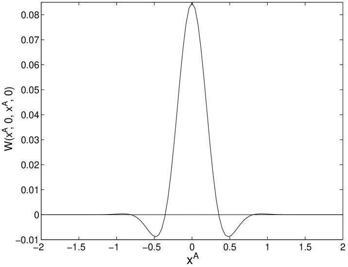
Figure 3: A one-dimensional cut of the Wigner function of the two-mode state $\rho_{c,AB}$ along the line $x^{B}=x^{A}$, $p^{A}=p^{B}=0$ for $\lambda=0.6$ and beam splitters BS_A and BS_B transmittances $T=0.95$. Notice the regions where $W$ is negative.

A necessary condition for the observation of a violation of Bell inequalities with homodyne detectors is that the Wigner function of the two-mode state used in the Bell test is not positive definite. Figure 3 illustrates that the Wigner function (25) of the conditionally generated state $\rho_{c,AB}$ is indeed negative in some regions of the phase space. The area of negativity, as well as the attained negative values of W, are rather small, which indicates that we should not expect a high Bell violation with homodyning.

As we have shown in Section II, the maximum Bell factor $S$ achievable with our setup and sign binning is about $S=2.048$. We conjecture that this binning is optimal or close to optimal. This is supported by the simple structure of the joint probability distribution (33). As can be seen in Fig. 4(a,b), $P$ exhibits two peaks, both located in the quadrants where Alice’s and Bob’s measured quadratures have the same sign. Note also that the two-peak structure is a clear signature of the non-Gaussian character of the state (c.f. Fig. 4(c,d)). We have carried out numerical calculations of $S$ for several other possible binnings which divide the quadrature axis into three or four intervals, and have not found any binning which would provide higher $S$ than the sign binning. We have also performed optimization over the angles $\theta_{j}$ and $\phi_{k}$ and all the results and figures presented in this Section were obtained for the optimal choice of angles $\theta_{1}=0$, $\theta_{2}=\pi/2$, $\phi_{1}=-\pi/4$, $\phi_{2}=\pi/4$.

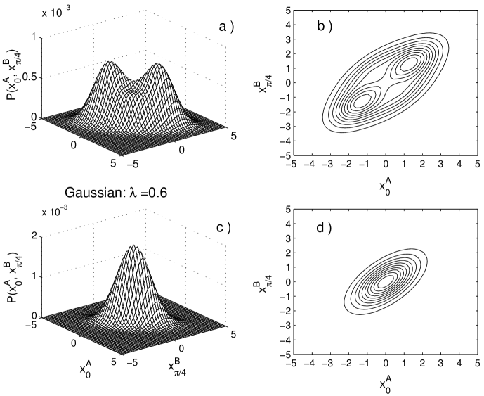
Figure 4: Joint probability distribution $P(x_{\theta_{j}}^{A},x_{\phi_{k}}^{B})$. Panels (a) and (b) show the distribution for the conditionally-prepared non-Gaussian state with $T=0.99$. Panels (c) and (d) display the distribution for the initial Gaussian two-mode squeezed vacuum state. The curves are plotted for perfect detectors $\eta_{\mathrm{PD}}=\eta_{\mathrm{BHD}}=100$%, squeezing $\lambda=0.6$ and $\theta_{\mathrm{Alice}}=0$ and $\phi_{\mathrm{Bob}}=\pi/4$.

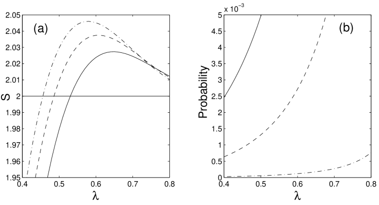
Figure 5: Violation of Bell-CHSH inequality with the conditionally-prepared non-Gaussian state. (a) Bell factor $S$ as a function of the squeezing. (b) Probability of success of the generation of the non-Gaussian state as a function of the squeezing. The curves are plotted for perfect detectors ($\eta_{\mathrm{\mathrm{PD}}}=\eta_{\mathrm{\mathrm{BHD}}}=100$%) with $T=0.9$ (solid line), $T=0.95$ (dashed line), and $T=0.99$ (dot-dashed line).

Figure 5(a) illustrates that the Bell-CHSH inequality $|S|\leq 2$ can be violated with the proposed set-up, and shows that there is an optimal squeezing $\lambda_{\mathrm{\mathrm{opt}}}$ which maximizes $S$. This optimal squeezing is well predicted by the simple model assuming perfect detectors with single-photon resolution (section II B), $\lambda_{\mathrm{\mathrm{opt}}}T\approx 0.57$. The curve plotted for $T=0.99$ practically coincides with the results obtained from the simple model presented in Sec. II B, c.f. Fig. 2(a). This confirms that in the limit $T\rightarrow 1$ the detectors with single-photon sensitivity become for our purposes equivalent to photodetectors with single-photon resolution. The maximum Bell factor achievable with our scheme is about $S_{\mathrm{max}}\approx 2.045$ which represents a violation of the Bell inequality by $2.2$%. To get close to the $S_{\mathrm{max}}$ one needs sufficiently high (but not too strong) squeezing. In particular, the value $\lambda\approx 0.57$ corresponds to approximately 5.6 dB of squeezing. Figure 5(b) illustrates that there is a clear trade-off between $S$ and the probability of success $P_{G}$. To maximize $S$ one should use highly transmitting beam splitters but this would reduce $P_{G}$. The optimal $T$ that should be chosen would clearly depend on the details of the experimental implementation.

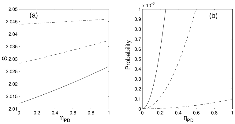
Figure 6: Effect of the inefficiency of the photodetectors PD_A and PD_B. (a) Bell parameter $S$ as a function of the efficiency $\eta_{\mathrm{PD}}$ of the photodetectors. (b) Probability of success as a function of the efficiency $\eta_{\mathrm{PD}}$. The curves are plotted for $T\lambda=0.57$, $\eta_{\mathrm{BHD}}=100\%$ and the same transmittances as in Fig. 5.

It follows from Fig. 6(a) that the Bell factor $S$ depends only very weakly on the efficiency $\eta_{\mathrm{PD}}$ of the single-photon detectors, so the Bell inequality can be violated even if $\eta_{\mathrm{PD}}\approx 1$%. This is very important from the experimental point of view because, although the quantum detection efficiencies of the avalanche photodiodes may be of the order of $50$%, the necessary spectral and spatial filtering which selects the mode that is detected by the photodetector may reduce the overall detection efficiency to a few percent. Low detection efficiency only decreases the probability of conditional generation $P_{G}$ of the non-Gaussian state, see Fig. 6(b). The dependence of $P_{G}$ on $\eta_{\mathrm{PD}}$ and $T$ can be very well approximated by a quadratic function, $P_{G}\approx\eta_{\mathrm{PD}}^{2}(1-T)^{2}$ which quickly drops when $\eta_{\mathrm{PD}}$ decreases. In practice, the minimum necessary $\eta_{\mathrm{PD}}$ will be determined mainly by the constraints on the total time of the experiment and by the dark counts of the detectors.

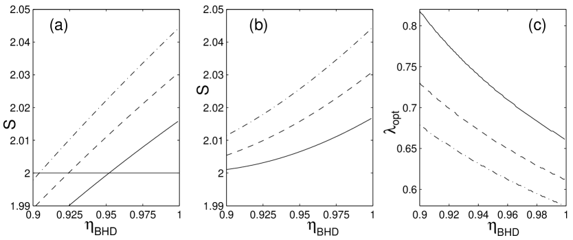
Figure 7: Effect of inefficient homodyning. (a) Bell parameter $S$ as a function of the efficiency $\eta_{\mathrm{BHD}}$ of the homodyning. The curve is plotted for $T\lambda=0.57$, $\eta_{\mathrm{PD}}=30\%$ and the same transmittances as in Fig. 5. (b) Bell parameter achieved for the optimal squeezing $\lambda_{\mathrm{opt}}$ is plotted as a function of $\eta_{\mathrm{BHD}}$. (c) Optimal squeezing $\lambda_{\mathrm{opt}}$ is plotted as a function of $\eta_{\mathrm{BHD}}$. The curve is plotted for $\eta_{\mathrm{PD}}=30\%$ and the same transmittances as in Fig. 5.

In contrast, the Bell factor $S$ strongly depends on the efficiency of the homodyne detectors, and $\eta_{\mathrm{\mathrm{BHD}}}$ must be above $\sim 90$% in order to observe Bell violation, see Fig. 7. However, this is not an obstacle because such (and even higher) efficiency has been already achieved experimentally (see e.g. zhang03 ). Interestingly, we have found that it is possible to partially compensate for imperfect homodyning with efficiency $\eta_{\mathrm{BHD}}<1$ by increasing the squeezing of the initial state. This effect is illustrated in Fig. 7(b) which shows the dependence of the Bell factor $S$ on $\eta_{\mathrm{BHD}}$ for optimal squeezing $\lambda_{\mathrm{opt}}$. Figure 7(c) then shows how the optimal squeezing increases with decreasing $\eta_{\mathrm{BHD}}$.

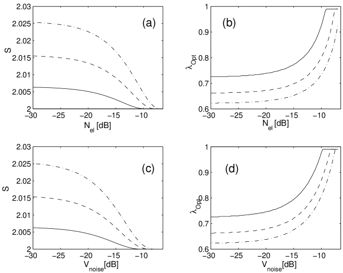
Figure 8: Effect of the electronic noise and thermal input states. (a) Maximum achievable Bell parameter $S$ with the optimal squeezing $\lambda_{\mathrm{opt}}$ as a function of the electronic noise $N_{\mathrm{el}}$. (b) Optimal squeezing $\lambda_{\mathrm{opt}}$ giving the highest Bell parameter $S$ for a given electronic noise. (c) Maximum Bell parameter $S$ as a function of the thermal noise of the input state $V_{\mathrm{noise}}$. (d) Optimal squeezing $\lambda_{\mathrm{opt}}$ giving the highest Bell parameter $S$ for a given thermal noise at the input. The curves are plotted for $\eta_{\mathrm{\mathrm{PD}}}=30$%, $\eta_{\mathrm{\mathrm{BHD}}}=95$%, and $T=0.9$ (solid line), $T=0.95$ (dashed line), and $T=0.99$ (dot-dashed line).

In addition to imperfect detection efficency $\eta_{\mathrm{BHD}}$, the electronic noise of the homodyne detector is another factor that may reduce the observed Bell violation. We model the added electronic noise by assuming that the effective quadrature that is detected $x_{\mathrm{det}}$ is related to the signal quadrature $x_{S}$ by a formula,

$$x_{\mathrm{det}}=\sqrt{\eta_{\mathrm{\mathrm{BHD}}}}\,x_{S}+\sqrt{1-\eta_{\mathrm{\mathrm{BHD}}}}\,x_{\mathrm{vac}}+\sqrt{N_{\mathrm{el}}}\,x_{\mathrm{noise}},$$

where $x_{\mathrm{vac}}$ and $x_{\mathrm{noise}}$ are two independent Gaussian distributed quadratures with zero mean and variance $1/2$, and $N_{\mathrm{el}}$ is the electronic noise variance expressed in shot noise units. On the level of covariance matrices, $N_{\mathrm{el}}$ can be included by modifying the formula for the noise matrix $G$ ,

$$G=(1-\eta_{\mathrm{\mathrm{BHD}}}+N_{\mathrm{el}})I_{AB}\oplus(1-\eta_{\mathrm{PD}})I_{CD}.$$ (41)

The homodyne detector with electronic noise is actually equivalent to a detector without noise but with a lower homodyne detector efficiency $\eta_{\mathrm{\mathrm{BHD}}}^{\prime}=\eta_{\mathrm{\mathrm{BHD}}}/(1+N_{\mathrm{el}})$. This can be shown by noting that the re-normalized quadrature $x_{\mathrm{det}}/\sqrt{1+N_{\mathrm{el}}}$ is exactly a quadrature that would be detected by a balanced homodyne detector with $N_{\mathrm{el}}=0$ and efficiency $\eta_{\mathrm{\mathrm{BHD}}}^{\prime}$. Our calculations reveal that the electronic noise should be $15-20$ dB below shot noise (see Fig. 8(a) and (b)), which is currently attainable with low-noise charge amplifiers. Again, higher squeezing can partially compensate for the increasing noise.

So far we have assumed that the source in Fig. 1 emits pure two-mode squeezed vacuum state. However, experimentally, it is very difficult to generate pure squeezed vacuum saturating the Heisenberg inequality. It is more realistic to consider a mixed Gaussian state such as squeezed thermal state which can be equivalently represented by adding quadrature independent Gaussian noise with variance $V_{\mathrm{noise}}$ to each mode of the two-mode squeezed vacuum. The effect of the added noise stemming from input mixed Gaussian state is quite similar to the influence of the electronic noise of the homodyne detector, see Fig. 8 (c) and (d). We find again that the added noise in the initial Gaussian state should be $15-20$ dB below the shot noise.

III.3 Four photon subtractions

Until now we have focused on a single-photon subtraction on each side (one photon removed from mode $A$ and one from mode $B$). If we now consider a scheme where two photons are subtracted from each mode, the de-gaussification of the state will be stronger and we may expect a higher Bell violation than before. To subtract two photons from each mode, we only need to add one more unbalanced beam splitter and photodetector on each side in Fig. 1. A successful state generation would be indicated by simultaneous clicks of all four detectors. Assuming perfect photon-number resolving detectors, the state generated from two-mode squeezed vacuum (3) by subtracting two photons from each mode can be expressed as

$$|\psi_{\mathrm{out}}\rangle_{AB} \propto a^{2}b^{2}|\psi_{\mathrm{in}}(T^{2}\lambda)\rangle_{AB}$$ (42)

$$\propto \sum_{n}(n+2)(n+1)(T^{2}\lambda)^{n}|n,n\rangle_{AB},$$

and the probability of success reads

$$P_{\mathrm{4ph}}=2T^{2}(1-T)^{4}\lambda^{4}(1-\lambda^{2})\frac{1+10T^{4}\lambda^{2}+T^{8}\lambda^{4}}{(1-T^{4}\lambda^{2})^{5}}.$$ (43)

Since the state (42) exhibits perfect photon number correlations, the Munro’s formula for the Bell factor can again be directly applied Munro99 . Numerical calculations show that the maximum Bell violation with the state (42) and sign binning of quadratures is achieved for $T^{2}\lambda=0.40$ which yields $S_{\mathrm{max,4ph}}=2.064$, which is indeed higher than the maximum achievable with two-photon subtraction, $S_{\mathrm{max,2ph}}=2.048$, and very close to the maximum value $S=2.076$ Munro99 .

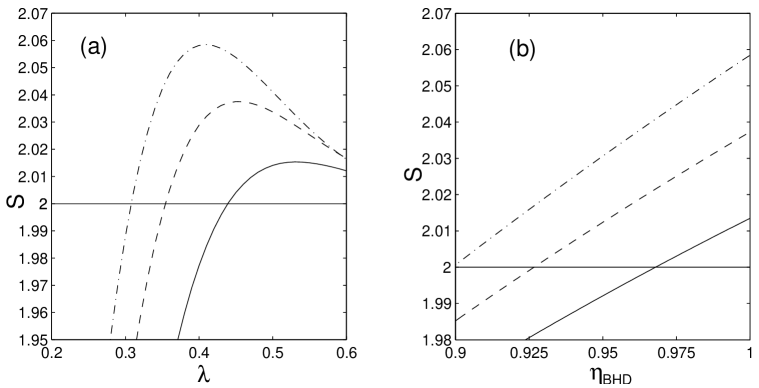
Figure 9: Violation of Bell-CHSH inequality with four photon subtractions. (a) Bell parameter $S$ as a function of the squeezing $\lambda$ for perfect detectors $\eta_{\mathrm{PD}}=\eta_{\mathrm{BHD}}=100$%. (b) Bell parameter $S$ as a function of the efficiency $\eta_{\mathrm{BHD}}$ of the homodyning. The curve is plotted for $T^{2}\lambda=0.40$, $\eta_{\mathrm{PD}}=100\%$ and the same transmittances as in Fig. 5.

A more realistic description of the four-photon subtraction scheme that takes into account realistic imperfect detectors can be developed using the approach described in detail in Sec. IIIB. We find that the Wigner function of the conditionally generated state is a linear combination of sixteen Gaussians. The results of numerical calculations are shown in Figs. 9(a) and (b), which illustrate that the two-photon subtraction from each mode yields higher violation of Bell-CHSH inequality than one-photon subtraction only for very high transmittances $T>0.95$. For lower transmittances, the fact that the photodetectors do not distinguish the number of photons reduces the Bell factor. Moreover, adding a second stage of photon subtractions dramatically decreases the probability of generating the non-Gaussian state. The probability can be estimated as $P_{G}\approx\eta_{\mathrm{PD}}^{4}(1-T)^{4}$, so for $T>0.95$ and $\eta=50$% we get $P_{G}\approx 10^{-6}$ and the duration of data acquisition would make the experiment infeasible. We conclude that from the practical point of view there seems to be no advantage in using the scheme with four photon subtractions instead of the much simpler scheme with two photon subtractions.

Figure 10: Symbol convention. (a) Single-mode squeezer along the $x$ quadrature. (b) Two-mode squeezer. (c) Beam splitter. (d) Conditional subtraction of a photon as described in the preceding section.

IV Alternative schemes

In this section we will study the violation of Bell-CHSH inequalities for a large group of alternative schemes, which involve from one to four photon subtractions. The main objective of this section is to compare the maximum Bell-CHSH factor $S$ obtained for the different proposed setups. As the main purpose of this section is the comparison of the different schemes, we will consider only idealized schemes with almost perfect single-photon subtraction on the beam splitters ($T=0.99$), and perfect photodetectors and homodyning ($\eta_{\mathrm{PD}}=\eta_{\mathrm{BHD}}=100$%). The maximum achievable Bell factor for each scheme presented below was determined by optimizing over the angles $\theta_{1,2}$, $\phi_{1,2}$ as well as over the squeezing $\lambda$ of the initial Gaussian states. The sign binning of the measured quadratures has been used in all cases. All the schemes presented in this section use the symbol convention depicted in Fig. 10.

In the preceding section, we have seen that the probability of successful generation of a non-Gaussian state decreases significantly with the number of photon subtractions. At the same time the complexity of the implementation of the experimental setup increases with the number of photon subtractions. It is then obvious that the most interesting schemes for a Bell-CHSH violation are those involving only one photon subtraction. Unfortunately, for the schemes that we have considered (see Fig. 11), no violation is observed.

Figure 11: Schemes with only one photon subtraction. The first column labels the different setups proposed, the second shows the scheme and finally the last column gives the maximal Bell factor $S$. (a) Photon subtraction after the creation of the two-mode squeezed vacuum. (b) Photon subtraction before mixing two single-mode squeezed states on a beam splitter.

After one photon subtraction, the simplest schemes are those with two photon subtractions. In the preceding sections it was shown that it is possible to violate Bell-CHSH inequality with two photon subtractions (scheme Fig. 12(a)). It follows from Fig. 12 that several other schemes (scheme Fig. 12(d) and (e)) also violate Bell-CHSH inequality but the maximal achievable Bell factor $S$ is much smaller in comparison to the scheme shown in Fig. 12(a).

Figure 12: Schemes with two photon subtractions. The right column gives the maximal value of the Bell factor $S$ for the proposed setups.

By adding one more photon subtraction to the schemes shown in Fig. 12, we can construct an ensemble of schemes with three photon subtractions. After numerical optimization we have found that none of these schemes succeeds to violate Bell-CHSH inequality. This striking result together with the the fact that we have not found any violation for schemes based on a single subtraction suggests that it may be necessary to have a scheme with an even number of photon subtractions in order to observe $S>2$.

In the preceding section, we have also proposed one scheme with four photon subtractions that violates Bell-CHSH inequality. Many other possible schemes exist where four photons are subtracted. Figure 13 illustrates some particular examples, which are based on the preparation of two-mode squeezed vacuum via mixing of two single-mode squeezed states on an balanced beam splitter. The photon subtractions are symmetrically placed to both modes. Strikingly, if all four photons are subtracted either before or after mixing on a beam splitter, then we get $S>2$. However, if a single photon is subtracted from each mode both before and after combining the modes on a beam splitter, then we do not obtain any Bell violation.

Figure 13: Schemes with four photon subtractions. Last column gives the maximal value of the Bell factor $S$ for the proposed setups.

Finally we have also studied an alternative group of schemes where instead of subtracting photons separately from modes $A$ and $B$, we mix the auxiliary modes $C$ and $D$ on a balanced beam splitter before the detection on the photodetectors. Consider the scheme depicted in Fig. 14(a) where only a single photon is subtracted. The mixing of modes $C$ and $D$ on a beam splitter erases the information about the origin of the detected photon which implies that the conditionally prepared state is a coherent superposition of states where a single photon has been removed either from mode $A$ or from mode $B$. However, even this modification does not lead to Bell violation with just a single subtraction.

We can extend the scheme by placing a photodetector at both output ports of the beam splitter, cf. Fig. 14(b). In the limit of a high transmittance $T\rightarrow 1$, the conditioning on the click of each detector selects the events where there were altogether two photons at the beam-splitter inputs. The bosonic properties of the photons imply that a simultaneous click of both photodetectors occurs only if the two subtracted photons are coming from the same mode ($A$ or $B$) Hong87 , but again we do not know from which mode the two photons are subtracted. This scheme is thus equivalent to the superposition of two schemes of the type shown in Fig. 12(c). Unlike the scheme in Fig. 12(c), the scheme in Fig. 14(b) is symmetric with respect to the modes $A$ and $B$. However, no violation can be observed. On the other hand, the scheme in Fig. 14(c) leads to $S>2$ by realizing a superposition of states where two photons are subtracted from a single-mode squeezed vacuum state and this state is then mixed with another single-mode squeezed vacuum on a balanced beam splitter, see 12(d). In comparison to the scheme in Fig. 12(d), we obtain much higher violation $S=2.046$.

Figure 14: Schemes consisting of superpositions of other schemes proposed above. (a) Superposition of one photon subtraction on modes $A$ or $B$. (b), (c) Superposition of two photon subtractions on modes $A$ or $B$.

V Conclusions

We have proposed an experimentally feasible setup allowing for a loophole-free Bell test with efficient homodyne detection using a non-gaussian entangled state generated from a two-mode squeezed vacuum state by subtracting a single photon from each mode. We have presented a full analytical description of a realistic setup with imperfect detectors, noise and mixed input states. We have studied in detail the influence of the detector inefficiencies, the electronic noise of homodyne detector, and the input mixed states, on the achievable Bell violation. The main feature of the present scheme is that it is largely insensitive to the detection efficiency of the avalanche photodiodes that are used for conditional preparation of the non-gaussian state, so that detector efficiencies of the order of a few per cent are sufficient. On the other hand, the detection efficiency of the balanced homodyne detector should be of the order of $90$% and the electronic noise of the homodyne detector should be at least $15$ dB below the shot noise level. The optimal squeezing that yields maximum Bell violation depends on the experimental circumstances but is, generally speaking, within the range of experimentally attainable values. As a rule, the optimal squeezing increases with decreasing $\eta_{\mathrm{\mathrm{BHD}}}$ and increasing noise.

We have also discussed several alternative schemes that involve the subtraction of one, two, three or four photons. The experimentally simplest and most appealing schemes are those where only a single photon is subtracted because photon subtraction is a delicate operation and also each subtraction in the scheme drastically reduces the probability of successful state generation. Unfortunately, we have not been able to find a scheme with only a single subtraction which would exhibit violation of Bell inequalities. However, the class of schemes that we have studied is still somewhat restricted. One can thus hope that such a scheme may be designed by considering more complicated setups involving unbalanced beam splitters and possibly a different binning procedure Eisert04private . This issue certainly deserves further investigation.

Among all the schemes where two photons are subtracted, the maximum violation $S=2.046$ is achieved by the scheme discussed in Sections II and III. Taking into account that we have not found any scheme with three photon subtractions which would violate Bell-CHSH inequality, the only way of exceeding the 2.046 violation appears to be by subtracting four photons. This scheme has been analyzed in some detail in Sec. IIIC where it was shown that this allows us to reach the Bell factor $S=2.06$. Unfortunately, the price to pay for this slight increase of $S$ is that the probability of successful conditional generation is so low that it makes the experiment infeasible.

The results presented in this paper provide a clear example of the utility of conditional photon subtraction which can be considered as an important novel tool in quantum optics and quantum information processing with continuous variables. Besides violation of Bell inequalities, this method can be used to generate highly non-classical states of light Wenger04 , to improve the fidelity of teleportation of continuous variable states Opatrny00 ; Cochrane02 ; Olivares03 and it forms a key ingredient of recently proposed entanglement purification protocols for continuous variables Browne03b ; Eisert04 . The very recent experimental demonstration of a single photon subtraction from a single-mode squeezed vacuum state provides a strong incentive for further theoretical and experimental developments along these lines, and we can thus expect that some of the schemes discussed in the present paper will be experimentally implemented in a not too distant future.

Note added: After this work was completed we have learned that a scheme for observing a violation of Bell inequalities similar to the scheme discussed in Sec. II of the present paper has been independently proposed by H. Nha and H.J. Carmichael Nha04 .

- (1) A. Einstein, B. Podolsky, and N. Rosen, Phys. Rev. 47, 777 (1935).
- (2) J. S. Bell, Physics (Long Island City, N.Y.) 1, 195 (1964).
- (3) S. J. Freedman and J. F. Clauser, Phys. Rev. Lett. 28, 938 (1972).
- (4) A. Aspect, P. Grangier, and G. Roger, Phys. Rev. Lett. 47, 460 (1981).
- (5) A. Aspect, P. Grangier, and G. Roger, Phys. Rev. Lett. 49, 91 (1982).
- (6) A. Aspect, J. Dalibard, and G. Roger, Phys. Rev. Lett. 49, 1804 (1982).
- (7) P. G. Kwiat, K. Mattle, H. Weinfurter, A. Zeilinger, A. V. Sergienko, and Y. Shih, Phys. Rev. Lett. 75, 4337 (1995).
- (8) G. Weihs, T. Jennewein, C. Simon, H. Weinfurter, and A. Zeilinger, Phys. Rev. Lett. 81, 5039 (1998).
- (9) M.A. Rowe, D. Kielpinski, V. Meyer, C.A. Sackett, W. M. Itano, C. Monroe, and D.J. Wineland, Nature (London) 409, 791 (2001).
- (10) W. Tittel, J. Brendel, B. Gisin, T. Herzog, H. Zbinden, and N. Gisin, Phys. Rev. A 57, 3229 (1998).
- (11) Philip M. Pearle, Phys. Rev. D 2, 1418 (1970).
- (12) P. G. Kwiat, P. H. Eberhard, A. M. Steinberg, and R. Y. Chiao, Phys. Rev. A 49, 3209 (1994).
- (13) E. Santos, Phys. Rev. A 46, 3646 (1992).
- (14) N. Gisin and B. Gisin, Phys. Lett. A 260, 323 (1999).
- (15) S. Massar, S. Pironio, J. Roland, and B. Gisin, Phys. Rev. A 66, 052112 (2002).
- (16) C. Simon and W.T.M. Irvine, Phys. Rev. Lett. 91, 110405 (2003).
- (17) X.-L. Feng, Z.-M. Zhang, X.-D. Li, S.-Q. Gong, and Z.-Z. Xu, Phys. Rev. Lett. 90, 217902 (2003).
- (18) L.M. Duan and H. J. Kimble, Phys. Rev. Lett. 90, 253601 (2003).
- (19) D.E. Browne, M.B. Plenio, and S.F. Huelga, Phys. Rev. Lett. 91, 067901 (2003)
- (20) B.B. Blinov, D.L. Moehring, L.M. Duan, and C. Monroe, Nature (London) 428, 153 (2004).
- (21) E.S. Fry, T. Walther, and S. Li, Phys. Rev. A 52, 4381 (1995).
- (22) M. Freyberger, P. K. Aravind, M. A. Horne, and A. Shimony, Phys. Rev. A 53, 1232 (1996).
- (23) E. S. Polzik, J. Carri, and H. J. Kimble, Phys. Rev. Lett. 68, 3020 (1992).
- (24) F. Grosshans, G. Van Assche, J. Wenger, R. Brouri, N. J. Cerf, Ph. Grangier, Nature (London) 421, 238 (2003).
- (25) Z. Y. Ou, S. F. Pereira, H. J. Kimble, and K. C. Peng, Phys. Rev. Lett. 68, 3663-3666 (1992).
- (26) C. Schori, J. L. Sørensen, and E. S. Polzik, Phys. Rev. A 66, 033802 (2002).
- (27) W. P. Bowen, R. Schnabel, P. K. Lam, and T. C. Ralph, Phys. Rev. A 69, 012304 (2004).
- (28) J. Eisert, S. Scheel, and M.B. Plenio, Phys. Rev. Lett. 89, 137903 (2002).
- (29) J. Fiurášek, Phys. Rev. Lett. 89, 137904 (2002).
- (30) G. Giedke and J.I. Cirac, Phys. Rev. A 66, 032316 (2002).
- (31) D.E. Browne, J. Eisert, S. Scheel, and M.B. Plenio, Phys. Rev. A 67, 062320 (2003).
- (32) J. Eisert, D. Browne, S. Scheel, and M.B. Plenio, Annals of Physics (NY) 311, 431 (2004).
- (33) K. Banaszek and K. Wódkiewicz, Phys. Rev. A 58, 4345 (1998).
- (34) Z.-B. Chen, J.-W. Pan, G. Hou, and Y.-D. Zhang, Phys. Rev. Lett. 88, 040406 (2002).
- (35) L. Mišta, Jr., R. Filip, and J. Fiurášek, Phys. Rev. A 65, 062315 (2002).
- (36) R. Filip and L. Mišta, Jr., Phys. Rev. A 66, 044309 (2002).
- (37) A. Gilchrist, P. Deuar, and M.D. Reid, Phys. Rev. Lett. 80, 3169 (1998).
- (38) A. Gilchrist, P. Deuar, and M.D. Reid, Phys. Rev. A 60, 4259 (1999).
- (39) W. J. Munro, Phys. Rev. A 59, 4197 (1999).
- (40) J. Wenger, M. Hafezi, F. Grosshans, R. Tualle-Brouri, and P. Grangier, Phys. Rev. A 67, 012105 (2003).
- (41) T. Opatrný, G. Kurizki, and D.-G. Welsch, Phys. Rev. A 61, 032302 (2000).
- (42) P.T. Cochrane, T.C. Ralph, and G.J. Milburn, Phys. Rev. A 65, 062306 (2002).
- (43) S. Olivares, M.G.A. Paris, and R. Bonifacio, Phys. Rev. A 67, 032314 (2003).
- (44) R. García-Patrón Sanchez, J. Fiurášek, N.J. Cerf, J. Wenger, R. Tualle-Brouri, and Ph. Grangier, quant-ph/0403191.
- (45) J. Wenger, R. Tualle-Brouri, and Ph. Grangier, Phys. Rev. Lett. 92, 153601 (2004).
- (46) J.S. Bell, Speakable and Unspeakable in Quantum Mechanics (Cambridge University Press, Cambridge, 1988) pp. 29 and 105.
- (47) J.F. Clauser, M.A. Horne, A. Shimony and R.A. Holt, Phys. Rev. Lett. 23, 880 (1969).
- (48) T. C. Zhang, K. W. Goh, C. W. Chou, P. Lodahl, and H. J. Kimble, Phys. Rev. A 67, 033802 (2003).
- (49) C. K. Hong, Z. Y. Ou, and L. Mandel, Phys. Rev. Lett. 59, 2044 (1987).
- (50) J. Eisert, private communication.
- (51) H. Nha and H.J. Carmichael, Phys. Rev. Lett. 93, 020401 (2004).