Controlling a group velocity of light by magnetic field

Abstract

We have shown that quantum interference in a driven quasi-degenerate two-level atomic system can be controlled by an externally applied magnetic field. We demonstrate that the mechanism of optical control is based on quantum interference, which allows one to implement both electromagnetically induced transparency and electromagnetically induced absorption in one atomic system. Dispersion of such the medium allows one to control group velocity of propagation of light pulses be ultra-slow or superluminal via applied magnetic field.

I Introduction

Quantum coherence and interference play an important role in the interaction of coherent laser fields with atomic systems. As has been shown that interplay between destructive and constructive interference of atomic transitions 1 leads to electromagnetically induced transparency (EIT) or electromagnetically induced absorption (EIA) 2 . EIT has found a wide variety of applications in quantum optics and nonlinear optical processes 3 . EIA could have potential applications to high-speed optical modulation and quantum switching 4 ; 5 .

$N$-type scheme has recently attracted much attention and opened a new approach to manipulate the nonlinear phenomena in optical process 6 . It has been shown that atomic coherence among Zeeman sublevels can be spontaneously transferred from upper level to lower one, which gives rise not only to EIT, but also to EIA 2 ; 7 ; 8 . Doppler-free resonance absorption observed in the $N$ scheme displays another interesting features in the Doppler-broadened medium 9 . Three-photon Doppler-free resonance has been observed in hot Rb vapor driven with one of two coherent fields far detuning from its resonance in the $N$ scheme10 . The other type of schemes have been analysed in Refs. 11 ; 12 .

Usually, the atomic system has one type of interference, either constructive or destructive, that depends on the configuration of atomic levels and laser fields. Recently, we show a way to coherently control the type of interference in one quasi-degenerate two-level atomic system by applying an external magnetic field 15 .

In this paper we show a possibility of control by means of magnetic field not only of the type of interference but of group velocity too. Application of magnetic field can change velocity of propagation of light pulses from ultra-slow to superluminal.

The paper is organized as follows. In Sec. II the physical model and the main equations are presented. The equations are solved in the stationary conditions. In Sec. III together with App. A the coherency is given for the thermal resonant medium. In Sec. IV the case of the immovable atoms in the N-cofiguration is investigated. At last, in Sec. V together with App. B the EIT, EIA and slow light effects are investigated in the thermal vapor.

II The physical model and the basic equations

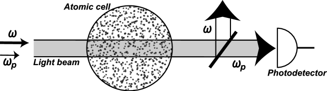
Figure 1: Experimental setup for observation of the EIT, EIA and slow light velocity effects

In Figure 1 the experimental setup discussed below is shown. It is assumed a light beam, consisting of two monochromatic waves, which are propagated into the same direction, with frequencies $\omega$ (the drive wave) and $\omega_{p}$ (the probe wave), passes through a cell of an atomic vapor at room temperature. It is assumed that each atom, participating in the thermal motion, crosses the light beam and after that looses any information about past interaction with light on the walls of cell. It means that any atom goes in into the light beam volume in a ground state ever independently of for the first time or otherwise.

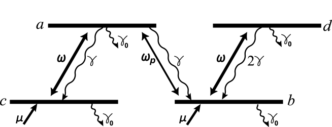
Figure 2: Schematic of N-type four-level system. Drive laser couples in the $(ac)$ and $(bd)$ transitions simultaneously, probe laser to $(ab)$

Let the atom has effectively a two-level energetic structure with a twice degeneration of both the levels (see fig. 2). In an outside magnetic field the Zeeman’s effect takes a place, and generally speaking it leads to respective splitting the levels. Let some conditions (for example, the light polarizations) ensure interactions of the drive field with the atom on both the $(ac)$- and $(bd)$- transitions and of the probe wave - on the $(ab)$-transition.

We take into account incoherent processes in the atomic system. First, there are spontaneous emissions on the $(ab)$- and $(ac)$-transitions with rates equaled to $\gamma$ and on the $(dc)$- transition - with $2\gamma$. Second, we model processes of arrival of atoms into the light beam volume and departure of them from there as incoherent processes too. As is seen in Fig. 2 there are a ”pump” with mean rate $\mu$ to the lower sub-levels and an additional ”decay” of all the sub-levels with rate $\gamma_{0}$.

We start with an equation for an atomic density matrix $\hat{\sigma}$ in the interaction picture for the single four-level atom, interacting with two coherent classical fields with complex amplitudes $\alpha$ (the drive field) and $\alpha_{p}$ (the probe field):

$$\dot{\hat{\sigma}}=-i\left[\hat{V},\hat{\sigma}\right]-\hat{R}\hat{\sigma}+\hat{\mu}.$$ (1)

The $\hat{R}$ and $\hat{\mu}$ operators ensure the mentioned above incoherent processes (see Fig. 2). The atom-field interaction Hamiltonian has a well known form:

$$\hat{V}=-g\alpha\mid a\rangle\langle c\mid e^{i\Delta_{1}t}-g\alpha\mid d\rangle\langle b\mid e^{i\Delta_{2}t}-g_{p}\alpha_{p}\mid a\rangle\langle b\mid e^{i\Delta_{p}t}+h.c.$$ (2)

Here are frequency detunings: $\Delta_{1}=\omega_{ac}-\omega,\;\Delta_{2}=\omega_{db}-\omega,\;\Delta_{p}=\omega_{ab}-\omega_{p}$ ($\omega_{ac},\;\omega_{bd}$ and $\omega_{ab}$ - the respective atomic frequencies).

Further we will use not the field amplitudes but the so-called Rabi-frequencies $\Omega=g\alpha$ and $\Omega_{p}=g_{p}\alpha_{p}$.

Rewriting the equation (1) in terms of matrix elements, we can obtain the following system of equations:

$$\dot{\sigma}_{aa}=-\left(2\gamma+\gamma_{0}\right)\sigma_{aa}+i\Omega_{p}\sigma_{ba}-i\Omega_{p}^{*}\sigma_{ab}+i\Omega\sigma_{ca}-i\Omega^{*}\sigma_{ac}=0$$ (3)

$$\dot{\sigma}_{bb}=\left(\mu+\gamma\sigma_{aa}\right)-\gamma_{0}\sigma_{bb}+2\gamma\sigma_{dd}-i\Omega_{p}\sigma_{ba}+i\Omega_{p}^{*}\sigma_{ab}+i\Omega^{*}\sigma_{db}-i\Omega\sigma_{bd}=0$$ (4)

$$\dot{\sigma}_{cc}=\mu-\gamma_{0}\sigma_{cc}+\gamma\sigma_{aa}+i\Omega^{*}\sigma_{ac}-i\Omega\sigma_{ca}=0$$ (5)

$$\dot{\sigma}_{dd}=-\left(2\gamma+\gamma_{0}\right)\sigma_{dd}+i\Omega\sigma_{bd}-i\Omega^{*}\sigma_{db}=0$$ (6)

and

$$\dot{\sigma}_{ab}=-\left(\gamma+\gamma_{0}+i\Delta_{p}\right)\sigma_{ab}+i\Omega_{p}\left(\sigma_{bb}-\sigma_{aa}\right)+i\Omega\sigma_{cb}-i\Omega\sigma_{ad}=0$$ (7)

$$\dot{\sigma}_{ca}=-\left(\gamma+\gamma_{0}-i\Delta_{1}\right)\sigma_{ca}-i\Omega_{p}^{*}\sigma_{cb}-i\Omega^{*}\left(\sigma_{cc}-\sigma_{aa}\right)=0$$ (8)

$$\dot{\sigma}_{ad}=-\left(2\gamma+\gamma_{0}+i\Delta_{p}-i\Delta_{2}\right)\sigma_{ad}+i\Omega_{p}\sigma_{bd}+i\Omega\sigma_{cd}-i\Omega^{*}\sigma_{ab}=0$$ (9)

$$\dot{\sigma}_{cb}=-\left(\gamma_{0}+i\Delta_{p}-i\Delta_{1}\right)\sigma_{cb}-i\Omega_{p}\sigma_{ca}+i\Omega^{*}\sigma_{ab}-i\Omega\sigma_{cd}=0$$ (10)

$$\dot{\sigma}_{bd}=-\left(\gamma+\gamma_{0}-i\Delta_{2}\right)\sigma_{bd}+i\Omega^{*}\left(\sigma_{dd}-\sigma_{bb}\right)+i\Omega_{p}^{*}\sigma_{ad}=0$$ (11)

$$\dot{\sigma}_{cd}=-\left(\gamma+\gamma_{0}+i\Delta_{p}-i\Delta_{1}-i\Delta_{2}\right)\sigma_{cd}+i\Omega^{*}\sigma_{ad}-i\Omega^{*}\sigma_{cb}=0$$ (12)

Under writing the equations the following replacements have been made:

$$\sigma_{ab}\to\sigma_{ab}e^{-i\Delta_{p}t}$$ (13)

$$\sigma_{ac}\to\sigma_{ac}e^{-i\Delta_{1}t}$$ (14)

$$\sigma_{db}\to\sigma_{db}e^{-i\Delta_{2}t}$$ (15)

$$\sigma_{ad}\to\sigma_{ad}e^{-i\left(\Delta_{p}-\Delta_{2}\right)t}$$ (16)

$$\sigma_{dc}\to\sigma_{dc}e^{-i\left(\Delta_{p}-\Delta_{1}-\Delta_{2}\right)t}$$ (17)

$$\sigma_{bc}\to\sigma_{bc}e^{-i\left(\Delta_{p}-\Delta_{1}\right)t}$$ (18)

We put all the derivatives equaled to zero because further only the stationary solutions are of our interest.

Now to make the mathematical situation simpler we remember interestingthat the probe wave is weak. It means we want to be restricted by the approximation $\Omega_{p}/(\gamma+\gamma_{0})\ll 1$ and to remain in our expressions only the main non-zero terms. As a result the wished coherencies read:

$$\sigma_{ab}=i\alpha_{p}\;\frac{1+if}{D}\left[n_{ba}+n_{ba}\;\frac{\mid\alpha\mid^{2}}{1+if}\left(\frac{1}{2-\varepsilon_{0}+if_{p2}}+\frac{1}{\varepsilon_{0}+if_{p1}}\right)-\right.$$

$$\left.-\;n_{ca}\;\frac{1}{1-if_{1}}\frac{\mid\alpha\mid^{2}}{\varepsilon_{0}+if_{p1}}+\;n_{db}\;\frac{1}{1-if_{2}}\frac{\mid\alpha\mid^{2}}{2-\varepsilon_{0}+if_{p2}}\right],$$ (19)

$$\sigma_{ca}=-n_{ca}\;\frac{i\alpha^{*}}{1-if_{1}},$$ (20)

$$\sigma_{bd}=-n_{bd}\;\frac{i\alpha^{*}}{1-if_{2}}.$$ (21)

The denominator $D$ in (19) is given by:

$$D=\left(1+if\right)\left(1+if_{p}\right)+\mid\alpha\mid^{2}\left(2+if_{p1}+if_{p2}\right)\left(\frac{1}{\varepsilon_{0}+if_{p1}}+\frac{1}{2-\varepsilon_{0}+if_{p2}}\right).$$ (22)

Here are the following notations:

$$n_{ik}=\sigma_{ii}-\sigma_{kk},\qquad i,k=a,b,c,d$$ (23)

$$f_{p}=\frac{\Delta_{p}}{\gamma(1+\varepsilon_{0})},\qquad f_{1}=\frac{\Delta_{1}}{\gamma(1+\varepsilon_{0})},\qquad f_{2}=\frac{\Delta_{2}}{\gamma(1+\varepsilon_{0}))},\qquad\varepsilon_{0}=\frac{\gamma_{0}}{\gamma+\gamma_{0}},$$ (24)

$$f_{p1}=f_{p}-f_{1},\qquad f_{p2}=f_{p}-f_{2},\qquad f=f_{p}-f_{1}-f_{2},\qquad f_{12}=f_{1}-f_{2}$$ (25)

$$\alpha_{p}=\frac{\Omega_{p}}{\gamma(1+\varepsilon_{0})},\qquad\alpha=\frac{\Omega}{\gamma(1+\varepsilon_{0})},\qquad\alpha_{0}=\frac{\alpha}{\sqrt{\varepsilon_{0}}},\qquad n_{0}=\frac{\mu}{\gamma_{0}}$$ (26)

Substituting (19-21) into (3-6) we obtain the closed system of equation for all the level populations. After relatively simple operations we are able to get the populations in the explicit form:

$$\sigma_{aa}=n_{0}\frac{2\mid\alpha\mid^{2}}{\left(2-\varepsilon_{0}\right)\left(1+f_{1}^{2}\right)+2\mid\alpha_{0}\mid^{2}\left(1+\varepsilon_{0}\right)}$$ (27)

$$\sigma_{bb}=n_{0}\frac{\left(2-\varepsilon_{0}\right)\left(1+f_{1}^{2}\right)+4\mid\alpha_{0}\mid^{2}}{\left(2-\varepsilon_{0}\right)\left(1+f_{1}^{2}\right)+2\mid\alpha_{0}\mid^{2}\left(1+\varepsilon_{0}\right)}\;\frac{\left(2-\varepsilon_{0}\right)\left(1+f_{2}^{2}\right)+2\mid\alpha\mid^{2}}{\left(2-\varepsilon_{0}\right)\left(1+f_{2}^{2}\right)+4\mid\alpha\mid^{2}}$$ (28)

$$\sigma_{cc}=n_{0}\frac{\left(2-\varepsilon_{0}\right)\left(1+f_{1}^{2}\right)+2\mid\alpha\mid^{2}}{\left(2-\varepsilon_{0}\right)\left(1+f_{1}^{2}\right)+2\mid\alpha_{0}\mid^{2}\left(1+\varepsilon_{0}\right)}$$ (29)

$$\sigma_{dd}=n_{0}\frac{\left(2-\varepsilon_{0}\right)\left(1+f_{1}^{2}\right)+4\mid\alpha_{0}\mid^{2}}{\left(2-\varepsilon_{0}\right)\left(1+f_{1}^{2}\right)+2\mid\alpha_{0}\mid^{2}\left(1+\varepsilon_{0}\right)}\;\frac{2\mid\alpha\mid^{2}}{\left(2-\varepsilon_{0}\right)\left(1+f_{2}^{2}\right)+4\mid\alpha\mid^{2}}$$ (30)

Substituting these formulas into (19)-(21) we can find all the coherencies in the explicit form and in particular the $\sigma_{ab}$ which is important for analysis of the optical properties of the $(ab)$-transition.

Further everywhere we will be restricted by the small value $\varepsilon_{0}\ll 1$. It means our requirement to the system is the passed lifetime of the atom through the light beam volume is much more than the lifetime of the upper laser state connected with spontaneous decay.

III The thermal motion of the atoms

As mentioned above our main goal here is to discuss the situation with the thermal motion of the atoms, forming the output signal under crossing the light beam volume. To describe correctly this case we have no right to use directly the previous formulas, because they are suitable in the obtained form only for the immovable atoms. But it is well known how to generalize it on the case of the thermal ensemble. We need to introduce by hands the available Doppler shifts, depending on velocities of the atoms, and then to average the formulas over the velocities with the adequate velocity distribution. In our conditions it means we have to make the following replacements in our formulas (19) and (27)-(30):

$$f_{p}\to f_{p}+x,\qquad f_{1}\to f_{1}+x,\qquad f_{2}\to f_{2}+x,\qquad f\to f-x$$ (31)

and then to average the obtained expressions with the Maxwell’s distribution:

$$W(x)=\frac{1}{\sqrt{\pi}x_{0}}e^{-x^{2}/x_{0}^{2}},\qquad x_{0}=\frac{ku}{\gamma},$$ (32)

where $ku$ is the Doppler spectral width of the absorption contour. In our approach we choose the so-called Doppler limit $x_{0}\gg 1$. One can find all the details of these operations in Appendix A.

After that we have to make additionally two things. First, we want to be restricted by case when the drive field frequency coincides with the atomic transition frequency in the absence of the magnetic field. Second, we have to introduce into the formulas the magnetic field in the explicit form. To satisfy this program we must make the following replacements in our formulas:

$$f_{1}\to 0,\qquad f_{2}\to-h,\qquad f_{p}\to f_{p}-h,\qquad f_{p1}\to f_{p}-h,\qquad f_{p2}\to f_{p},\qquad f\to f_{p}$$ (33)

where $h$ is the Zeeman shift of the $(b)$-level.

These operations are carried out in Appendix B.

IV Atoms at rest

In this section we will discuss the case of the immovable atoms. We think this can be interesting and useful for understanding the situation as whole.

According to (19) we can write the coherency for the $(ab)$-transition as the sum of three terms:

$$\sigma_{ab}=\sigma_{ab}^{ab}+\sigma_{ab}^{ac}+\sigma_{ab}^{bd},$$ (34)

connected respectively with the population differences $n_{ab},\;n_{ac}$ and $n_{bd}$ and having the following explicit forms:

$$\sigma_{ab}^{ab}=i\alpha_{p}n_{0}\;\frac{1+if_{p}-2if_{1}}{D}\;\frac{1+f_{1}^{2}+2\mid\alpha_{0}\mid^{2}}{1+f_{1}^{2}+\mid\alpha_{0}\mid^{2}}\;\frac{1+\left(f_{1}-ih\right)^{2}+\mid\alpha\mid^{2}}{1+\left(f_{1}-ih\right)^{2}+2\mid\alpha\mid^{2}}\times$$

$$\left[1+\frac{\mid\alpha\mid^{2}}{1+if_{p}-2if_{1}}\left(\frac{1}{\varepsilon_{0}+if_{p1}}+\frac{1}{2+if_{p1}+ih}\right)\right],$$ (35)

$$\sigma_{ab}^{ac}=-i\alpha_{p}\;n_{0}\frac{1+if_{p}-2if_{1}}{D}\;\frac{1+if_{1}}{1+f_{1}^{2}+\mid\alpha_{0}\mid^{2}}\;\frac{\mid\alpha\mid^{2}}{\varepsilon_{0}+if_{p1}},$$ (36)

$$\sigma_{ab}^{db}=-i\alpha_{p}n_{0}\;\frac{1+if_{p}-2if_{1}}{D}\;\frac{1+f_{1}^{2}+2\mid\alpha_{0}\mid^{2}}{1+f_{1}^{2}+\mid\alpha_{0}\mid^{2}}\;\frac{1+if_{1}-ih}{1+\left(f_{1}-ih\right)^{2}+2\mid\alpha\mid^{2}}\times$$

$$\frac{\mid\alpha\mid^{2}}{2+if_{p1}+ih},$$ (37)

where

$$D=\left(1+if_{p}-2if_{1}\right)\left(1+if_{p}-ih\right)+\mid\alpha\mid^{2}\left(2+2if_{p1}+ih\right)\times$$

$$\left(\frac{1}{\varepsilon_{0}+if_{p1}}+\frac{1}{2+if_{p1}+ih}\right)$$ (38)

These equations describe the absorption $Im(\sigma_{ab})$ and dispersion $Re(\sigma_{ab})$ of the probe wave interacting with $(ab)$-transition.

Here we have introduced the external magnetic field in the explicit form. We have put in the absence of the magnetic field the upper and lower levels are quite degenerated. It means the frequency shifts of the drive wave relative to both the transitions $(ac)$ and $(bd)$ are the same, that is $f_{1}=f_{2}$. For simplicity we have assumed that in the magnetic field only the $(b)$-level moves. Then $f_{2}=f_{1}-h$, where $h$ - is the Zeeman’s shift of the $(b)$-level.

The formulas (34)-(38) can be rewritten in the regime of the saturation by the drive field $\mid\alpha\mid,\mid\alpha_{0}\mid\gg 1$ in the simpler and more visible form. In resonant drive tuning $f_{1}=0$ and with the high power of the external magnetic field $(h\gg 1)$ the absorptive and dispersive contours read:

$$Re\left(\sigma_{ab}/\left(\alpha_{p}n_{0}\right)\right)=\frac{2\left(f_{p}-h-\mid\alpha\mid\right)}{1+4\left(f_{p}-h-\mid\alpha\mid\right)^{2}}+\frac{2\left(f_{p}-h+\mid\alpha\mid\right)}{1+4\left(f_{p}-h+\mid\alpha\mid\right)^{2}}$$ (39)

$$Im\left(\sigma_{ab}/\left(\alpha_{p}n_{0}\right)\right)=\frac{1}{1+4\left(f_{p}-h-\mid\alpha\mid\right)^{2}}+\frac{1}{1+4\left(f_{p}-h+\mid\alpha\mid\right)^{2}}$$ (40)

One can see these results can be interpreted as the dynamical Stark effect for three-level atom. Really, here the initial Lorenzian (or dispersive curve) with the zero drive field, placed on $f_{p}=h$, is split in the non-zero drive field on the two ones, placed on the horizontal axis symmetrically relative to $f_{p}=h$ on the frequencies $h\pm|\alpha|$. This effect is very clear because under the essential drift of the $(b)$-level the $(d)$-level falls simply out of the interaction with the drive field and so effectively the four-level atom is converted into the three-level one.

To the contrary, without the magnetic field $(h=0)$ all the four levels take an important role. The spectral contours in the case are given as:

$$Re\left(\sigma_{ab}/\left(\alpha_{p}n_{0}\right)\right)=\frac{f_{p}}{1+f_{p}^{2}}+\frac{1}{2}\;\frac{f_{p}-2\mid\alpha\mid}{1+\left(f_{p}-4\mid\alpha\mid\right)^{2}}+\frac{1}{2}\;\frac{f_{p}+2\mid\alpha\mid}{1+\left(f_{p}+4\mid\alpha\mid\right)^{2}}$$ (41)

$$Im(\sigma_{ab}/(\alpha_{p}n_{0}))=\frac{1}{1+f_{p}^{2}}+\frac{1}{2}\;\frac{1}{1+\left(f_{p}-4\mid\alpha\mid\right)^{2}}+\frac{1}{2}\;\frac{1}{1+\left(f_{p}+4\mid\alpha\mid\right)^{2}}$$ (42)

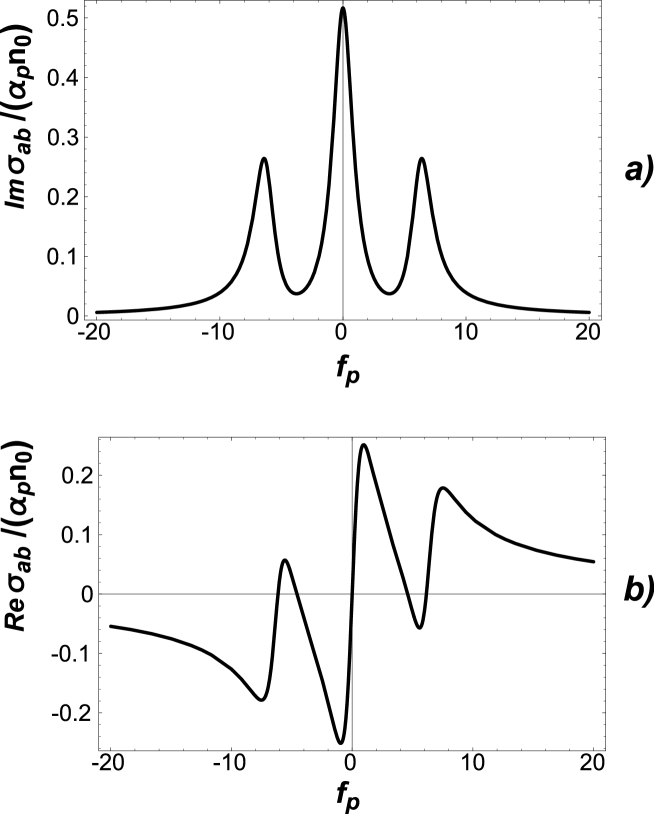
Figure 3: Frequency dependence of the imaginary $a)$ and real $b)$ parts of $\sigma_{ab}$ with $h=0$ and $|\alpha|^{2}=10$ for the immovable four-level atoms

Now there are three Lorencians in (41) (or three dispersive curves in (42)) instead of two in the previous situation. This difference is easy understood on the qualitative level under applying the model of the Rabi-splitting of levels. Without the magnetic field (the N-configuration for the four-level atom) both levels $(a)$ and $(b)$ are split, that gives three spectral contours instead of one. At the same time, in the strong magnetic field only the $(a)$-level is split, what ensures only two contours. In Fig. 3 the formulas (41)-(42) are presented graphically with $\mid\alpha\mid^{2}=10$.

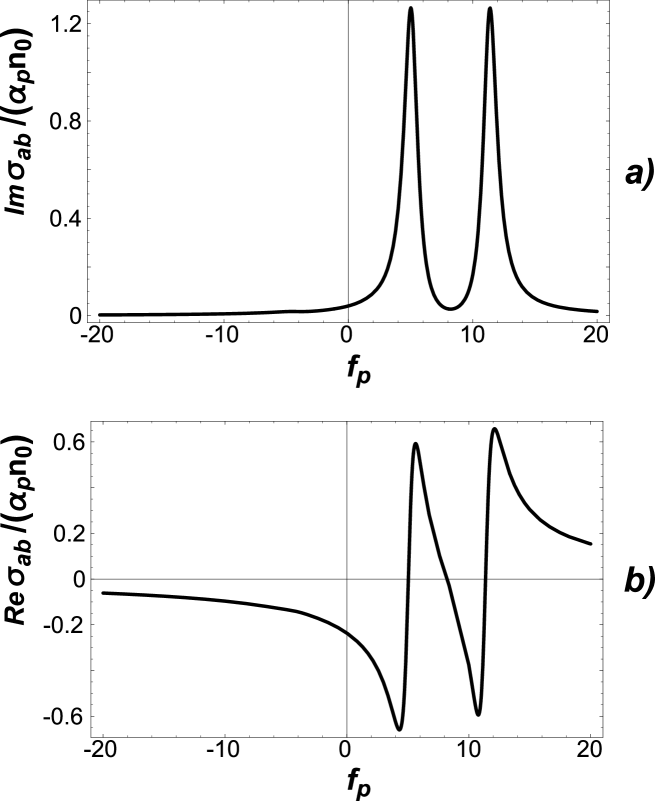
Figure 4: Frequency dependence of the imaginary $a)$ and real $b)$ parts of $\sigma_{ab}$ with $h=7$ and $|\alpha|^{2}=10$ for the immovable four-level atoms

At the same time, as stated above in the non-zero magnetic field we must expect a gradual transformation of the four-level atom into the three-level one. In Fig. 4 the curves are drown with $h=7,\;\varepsilon_{0}=1/10,\;\mid\alpha\mid^{2}=10$. One can see already with not very strong magnetic field the curves in the main match to the three-level structure in $\Lambda$-configuration.

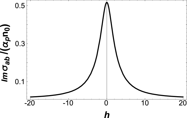
Figure 5: Dependence of the absorption of the immovable atoms on the magnetic field $h$ in the EIT-EIA area $f_{p}=h$

The EIT effect is available as we remember for the three-level atom. In consequence of the Rabi splitting in the strong drive field the center of the spectral contour turns out just between two peaks that is in the transparency area. Because in our case under gradual raising the magnetic field the three-level atom is achieved we can expect the stronger magnetic field, the better EIT. This is demonstrated in Fig. 5. There we watch over the center of the spectral contour $f_{p}=h$ and show, how this point falls in relation to $h$.

One can see the EIT effect takes a place even in the zero magnetic field (h=0) and the effect raises with $h$ as it was expected. The EIT effect with $h=0$ corresponds to falling the central point of the absorption contour in the strong drive field (see Fig. 3).

V The non-linear interference effects in the N-configuration

V.1 The EIA, EIT effects in the atomic vapor

Now let us discuss the experimental situation with the thermal ensemble of the atoms. In Sec. III it has been described, how to get the available formulas for this case. In App. A and B this program has been implemented.

In this section we are going to discuss some interesting details in the behaviour of the coherency $\sigma_{ab}$ in relation to the drive field and the externally applied magnetic field. Our consideration will be based on numerical calculations by the formulas (68)-(77), which have been given for the case of exact frequency tuning the drive field ($f_{1}=0$).

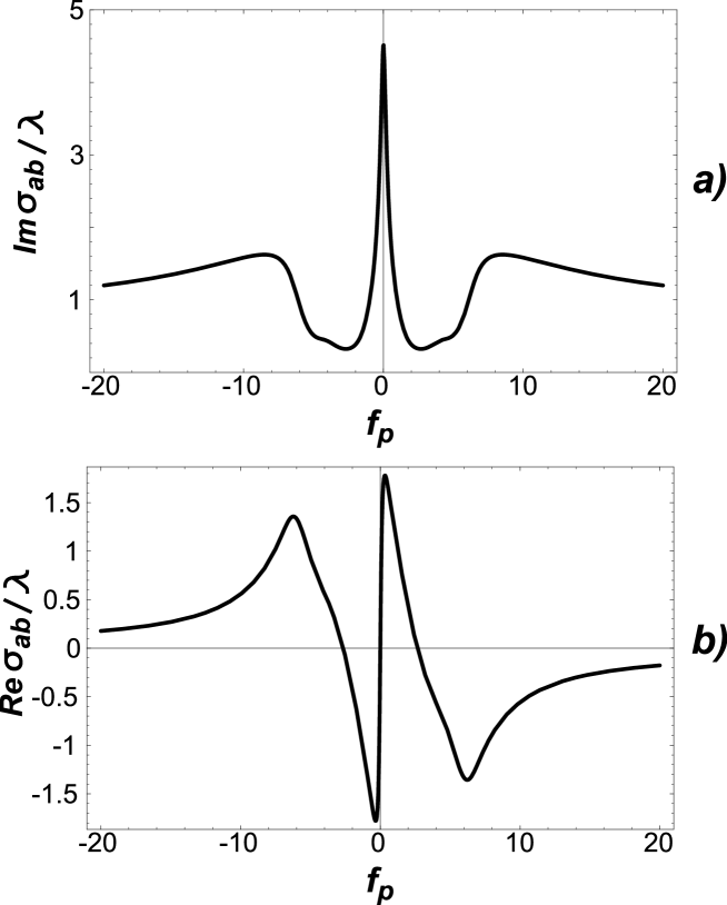
Figure 6: Frequency dependence of the imaginary $a)$ and real $b)$ parts of $\sigma_{ab}$ with $h=0$ and $|\alpha|^{2}=10,\;\varepsilon_{0}=1/10$ for the thermal four-level atoms, $\lambda=\alpha_{p}n_{0}\sqrt{\pi}/x_{0}$

First of all, let us discuss the absorptive properties of the vapor relative to the probe field. This is determined by the imaginary part of the coherency $\sigma_{ab}$, and this is presented in Fig. 6a for the zero magnetic field $h=0$ and with $x_{0}=100,\;\varepsilon_{0}=1/10,\;\mid\alpha_{0}\mid=10$.

Everywhere further we discuss not the density matrix itself but the value $\sigma/\lambda$. The factor $\lambda$ is chosen so to normalize this value onto one for the zero drive field in the contour center. So one can conclude the absorption with the strong drive field in the point $f_{p}=0$ is much more (with factor about 5) than without the drive field. It means in the zero magnetic field the N-configuration ensures the essential EIA effect.

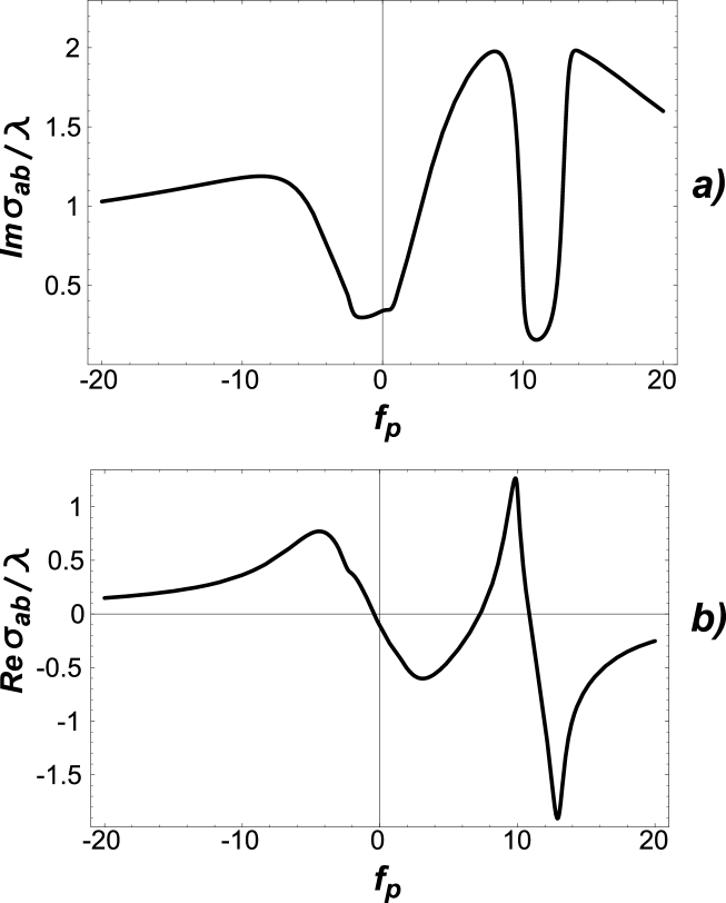
Figure 7: Frequency dependence of the imaginary $a)$ and real $b)$ parts of $\sigma_{ab}$ with $h=10$ and $|\alpha|^{2}=10,\;\varepsilon_{0}=1/10$ for the thermal four-level atoms

At the same time for the high enogh magnetic field in the point $f_{p}=h$ already the EIT effect takes a place. It is demonstrated in Fig. 7a for case $h=10$. One can see in the point $f_{p}=10$ the absorption is much less than one (about 0,165).

As a result we can conclude in the N-configuration we have a possibility to control an interference changing it by the externally applied magnetic field from distructive to constructive and back.

V.2 The slow light effect in the atomic vapor

Let us discuss now dispersive properties of the vapor on the $(ab)$-transition. For that we need to investigate the real part of the matrix element $\sigma_{ab}$. The respective frequency dependences are presented in Fig. 6b for the zero magnetic field $(h=0)$ and in Fig. 7b for $h=10$.

The interesting areas connect with a big derivatives with respect to $f_{p}(\omega_{p})$. Just there we can expect essential slowing the light pulse down. In the zero magnetic field (Fig. 6b) this is in the area near the zero frequency. At the same time with $h=10$ this is in the area near $f_{p}=10$ $(f_{p}=h)$. But the effect in the zero magnetic field (on the zero frequency) is bad for observation, because here the very effective absorption takes a place (compare with Fig. 6a).

At the same time, in the magnetic field (Fig. 7b) in the vicinity of $f_{p}=10$, where the good EIT effect takes a place, the derivative with respect to $f_{p}$ is high enough too. Taking this into account further we will analyze the group velocity of the light pulse as the function of the magnetic field in this area.

As is known the group velocity $v_{gr.}$ can be expressed via a real part of the susceptibility $\chi=Re\chi+iIm\chi$ as:

$$\frac{v_{gr.}}{c}=\left[1+2\pi\left(1+\omega_{p}\frac{d}{d\omega_{p}}\right)Re\chi\right]^{-1}$$ (43)

Rewriting it in terms of the density matrix and in our notations the formula reads:

$$\frac{v_{gr.}}{c}=\left[1+{\cal A}\left(1-\frac{\omega_{p}}{\gamma}\frac{d}{df_{p}}\right)Re\sigma_{ab}\right]^{-1},\qquad{\cal A}=\frac{3}{16\pi^{2}}\lambda_{p}^{3}N\frac{\gamma_{rad.}}{\gamma}\frac{1}{\mid\alpha\mid}$$ (44)

Here $\lambda_{p}$ and $\omega_{p}$ are the wavelength and the frequency of the probe field, $N$ is the atomic concentration, $\gamma_{rad.}$ is the constant of the radiation decay. For a numerical calculation we choose the following set of the parameters: $\lambda_{p}\sim~{}10^{-4}cm,\;N\sim~{}10^{12}cm^{-3},\;\gamma_{rad.}/\gamma\sim~{}1,\;\omega_{p}/\gamma\sim~{}{10}^{8},\;|\alpha_{p}/\alpha|\sim 10^{-1}$.

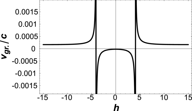
Figure 8: Dependence of the group velocity on the power of the externally applied magnetic field in the EIT/EIA area ($f_{p}=h$) with $|\alpha|^{2}=10,\;\varepsilon_{0}=1/10$

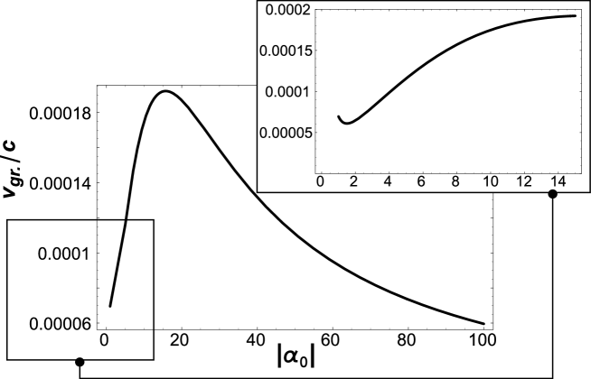
Figure 9: Dependence of the group velocity on the power of the drive field in the EIT area ($f_{p}=h=10$) with $\varepsilon_{0}=1/10$

In Fig. 8 the dependence of the group velocity in the vicinity of $f_{p}=h$ (the EIA or EIT area) on the magnetic field $h$ is presented with $|\alpha_{0}|=10$. As was expected the minimum of the velocity is achieved in the zero magnetic field. But we remember the light here is strongly absorbed on the transition. At the same time, with $h>5$ there is a slow light effect too, and there $v_{gr.}\sim 10^{-4}c$. This depends actually on the power of the drive field. One can see in Fig. 9 with $f_{p}=h=10$ at first the group velocity increases with changing the amplitude $\alpha_{0}$ from small to higher meanings, passes the maximum and next falls.

In conclusion, we have proposed effective coherent control of the optical properties of the resonant thermal medium. Varying the external magnetic field we can achieve in the same experiment both the EIT and EIA effects and also slow down light or to the contrary accelerate.

Appendix A Thermal motion of atoms

To take into account thermal motion of atoms we should make the following frequency replacements in our formulas:

$$f_{p}\to f_{p}+x,\qquad f_{1}\to f_{1}+x,\qquad f_{2}\to f_{2}+x,\qquad f=\to f-x$$ (45)

$$(f_{p1}=f_{p}-f_{1}\to f_{p1},\qquad f_{p2}=f_{p}-f_{2}\to f_{p2},\qquad f_{12}=f_{1}-f_{2}\to f_{12})$$

and then to average the formulas over $x$ with the Maxwell’s distribution:

$$W(x)=\frac{1}{\sqrt{\pi}x_{0}}e^{-x^{2}/x_{0}^{2}},\qquad x_{0}=\frac{ku}{\gamma}$$ (46)

After these operations in the Doppler limit ($x_{0}\gg 1$) the coherency, normalized on unity in the center of line of absorption with the zero driving field $\mid\alpha\mid$, is represented as the sum of terms:

$$\sigma_{ab}/\lambda=\sigma_{ab}^{ab}/\lambda+\sigma_{ab}^{ac}/\lambda+\sigma_{ab}^{bd}/\lambda,\qquad\lambda=\alpha_{p}n_{0}\sqrt{\pi}/x_{0}$$ (47)

where

$$\sigma_{ab}^{ab}/\lambda=A_{1}+A_{2}+A_{3}+A_{4}+A_{5}$$ (48)

$$A_{1}=\frac{1}{\pi}\int_{-\infty}^{+\infty}e^{-x^{2}/x_{0}^{2}}\frac{1}{x+f_{p}-i}\;\frac{1+\left(f_{1}+x\right)^{2}+2\mid\alpha_{0}\mid^{2}}{1+\left(f_{1}+x\right)^{2}+\mid\alpha_{0}\mid^{2}}\;dx=A_{1}^{\prime}+iA_{1}^{\prime\prime}$$ (49)

$$A_{2}=-\;\mid\alpha\mid^{2}\left(2+if_{p1}+if_{p2}\right)\left(\frac{1}{\varepsilon_{0}+if_{p1}}+\frac{1}{2+if_{p2}}\right)\frac{1}{\pi}e^{-f_{p}^{2}/x_{0}^{2}}\times$$

$$\int_{-\infty}^{+\infty}\frac{1}{x+f_{p}-i}\;\frac{1+\left(f_{1}+x\right)^{2}+2\mid\alpha_{0}\mid^{2}}{1+\left(f_{1}+x\right)^{2}+\mid\alpha_{0}\mid^{2}}\;\frac{1}{\left(x-x_{1}\right)\left(x-x_{2}\right)}\;dx$$ (50)

$$A_{3}=i\mid\alpha\mid^{2}\left(\frac{1}{\varepsilon_{0}+if_{p1}}+\frac{1}{2+if_{p2}}\right)\frac{1}{\pi}e^{-f_{p}^{2}/x_{0}^{2}}\times$$

$$\int\limits_{-\infty}^{+\infty}\frac{1+\left(f_{1}+x\right)^{2}+2\mid\alpha_{0}\mid^{2}}{1+\left(f_{1}+x\right)^{2}+\mid\alpha_{0}\mid^{2}}\;\frac{1}{\left(x-x_{1}\right)\left(x-x_{2}\right)}dx$$ (51)

$$A_{4}=-i\mid\alpha\mid^{2}\frac{1}{\pi}e^{-f_{p}^{2}/x_{0}^{2}}\times$$

$$\int_{-\infty}^{+\infty}\frac{1+\left(f_{1}+x\right)^{2}+2\mid\alpha_{0}\mid^{2}}{1+\left(f_{1}+x\right)^{2}+\mid\alpha_{0}\mid^{2}}\;\frac{1+i\left(f-x\right)}{\left(x-x_{1}\right)\left(x-x_{2}\right)}\frac{1}{1+\left(f_{2}+x\right)^{2}+2\mid\alpha\mid^{2}}dx$$ (52)

$$A_{5}=-i\mid\alpha\mid^{4}\left(\frac{1}{\varepsilon_{0}+if_{p1}}+\frac{1}{2+if_{p2}}\right)\frac{1}{\pi}e^{-f_{p}^{2}/x_{0}^{2}}\times$$

$$\int_{-\infty}^{+\infty}\frac{1+\left(f_{1}+x\right)^{2}+2\mid\alpha_{0}\mid^{2}}{1+\left(f_{1}+x\right)^{2}+\mid\alpha_{0}\mid^{2}}\;\frac{1}{\left(x-x_{1}\right)\left(x-x_{2}\right)}\frac{1}{1+\left(f_{2}+x\right)^{2}+2\mid\alpha\mid^{2}}dx$$ (53)

$$\sigma_{ab}^{ac}/\lambda=-\;\frac{\mid\alpha\mid^{2}}{\varepsilon_{0}+if_{p1}}\;\frac{1}{\pi}e^{-f_{p}^{2}/x_{0}^{2}}\times$$

$$\int_{-\infty}^{+\infty}\frac{x-f+i}{\left(x-x_{1}\right)\left(x-x_{2}\right)}\frac{1+i\left(f_{1}+x\right)}{1+\left(f_{1}+x\right)^{2}+\mid\alpha_{0}\mid^{2}}\;\;dx$$ (54)

$$\sigma_{ab}^{bd}/\lambda=-i\;\frac{\mid\alpha\mid^{2}}{2+if_{p2}}\;\frac{1}{\pi}e^{-f_{p}^{2}/x_{0}^{2}}\times$$

$$\int\limits_{-\infty}^{+\infty}\frac{1}{\left(x-x_{1}\right)\left(x-x_{2}\right)}\;\frac{\left(1-ix+if\right)\left(1+if_{2}+ix\right)}{1+\left(f_{2}+x\right)^{2}+2\mid\alpha\mid^{2}}\;\frac{1+\left(f_{1}+x\right)^{2}+2\mid\alpha_{0}\mid^{2}}{1+\left(f_{1}+x\right)^{2}+\mid\alpha_{0}\mid^{2}}dx$$ (55)

Here

$$x_{1,2}=-\;\frac{1}{2}\left(f_{1}+f_{2}\right)\pm\frac{i}{2}\left(2+if_{p1}+if_{p2}\right)\sqrt{1+\frac{4\mid\alpha\mid^{2}}{\left(\varepsilon_{0}+if_{p1}\right)\left(2+if_{p2}\right)}}$$ (56)

are the roots of the quadratic relative to $x$ equation

$$\left(1+if-ix\right)\left(1+if_{p}+ix\right)+\mid\alpha\mid^{2}\left(2+if_{p1}+if_{p2}\right)\left(\frac{1}{\varepsilon_{0}+if_{p1}}+\frac{1}{2+if_{p2}}\right)=0$$ (57)

Now we are able to carry out all integrations of the values of the complex resudues and obtain the following formulas expressed via the physical parameters in the explicit forms :

$$\sigma_{ab}^{ab}/\lambda=A_{1}+A_{2}+A_{3}+A_{4}+A_{5},$$ (58)

$$Re\left(A_{1}\right)=\frac{1}{\pi}\int_{-\infty}^{+\infty}e^{-x^{2}/x_{0}^{2}}\frac{x+f_{p}}{\left(x+f_{p}\right)^{2}+1}\;\frac{1+\left(f_{1}+x\right)^{2}+2\mid\alpha_{0}\mid^{2}}{1+\left(f_{1}+x\right)^{2}+\mid\alpha_{0}\mid^{2}}\;dx$$ (59)

$$Im\left(A_{1}\right)=e^{-f_{p}^{2}/x_{0}^{2}}\times$$

$$\left[\frac{f_{p1}\left(f_{p1}-2i\right)+2\mid\alpha_{0}\mid^{2}}{f_{p1}\left(f_{p1}-2i\right)+\mid\alpha_{0}\mid^{2}}+\frac{\mid\alpha_{0}\mid^{2}}{\sqrt{1+\mid\alpha_{0}\mid^{2}}\left[f_{p1}\left(f_{p1}+2i\sqrt{1+\mid\alpha_{0}\mid^{2}}\right)-\mid\alpha_{0}\mid^{2}\right]}\right]$$ (60)

$$A_{2}=\mid\alpha\mid^{2}\left(2+if_{p1}+if_{p2}\right)\left(\frac{1}{\varepsilon_{0}+if_{p1}}+\frac{1}{2+if_{p2}}\right)e^{-f_{p}^{2}/x_{0}^{2}}\times$$

$$\left[\frac{\mid\alpha_{0}\mid^{2}}{\sqrt{1+\mid\alpha_{0}\mid^{2}}\left(i\sqrt{1+\mid\alpha_{0}\mid^{2}}-f_{p1}+i\right)\left(i\sqrt{1+\mid\alpha_{0}\mid^{2}}+f_{1}+x_{1}\right)\left(i\sqrt{1+\mid\alpha_{0}\mid^{2}}+f_{1}+x_{2}\right)}+\right.$$

$$\left.+\;\frac{1+\left(f_{1}+x_{2}\right)^{2}+2\mid\alpha_{0}\mid^{2}}{1+\left(f_{1}+x_{2}\right)^{2}+\mid\alpha_{0}\mid^{2}}\;\frac{2i}{\left(x_{2}+f_{p}-i\right)\left(x_{2}-x_{1}\right)}\right]$$ (61)

$$A_{3}=-2\mid\alpha\mid^{2}\left(\frac{1}{\varepsilon_{0}+if_{p1}}+\frac{1}{2+if_{p2}}\right)e^{-f_{p}^{2}/x_{0}^{2}}\left[\frac{1+\left(f_{1}+x_{1}\right)^{2}+2\mid\alpha_{0}\mid^{2}}{1+\left(f_{1}+x_{1}\right)^{2}+\mid\alpha_{0}\mid^{2}}\;\frac{1}{\left(x_{1}-x_{2}\right)}+\right.$$

$$\left.+\;\frac{\mid\alpha_{0}\mid^{2}}{2i\sqrt{1+\mid\alpha_{0}\mid^{2}}\left(i\sqrt{1+\mid\alpha_{0}\mid^{2}}-f_{1}-x_{1}\right)\left(i\sqrt{1+\mid\alpha_{0}\mid^{2}}-f_{1}-x_{2}\right)}\right]$$ (62)

$$A_{4}=2\mid\alpha\mid^{2}e^{-f_{p}^{2}/x_{0}^{2}}\left[\frac{1+\left(f_{1}+x_{1}\right)^{2}+2\mid\alpha_{0}\mid^{2}}{1+\left(f_{1}+x_{1}\right)^{2}+\mid\alpha_{0}\mid^{2}}\;\frac{1+if-ix_{1}}{x_{1}-x_{2}}\;\frac{1}{1+\left(f_{1}+x_{2}\right)^{2}+2\mid\alpha\mid^{2}}+\right.$$

$$\left.+\frac{\mid\alpha_{0}\mid^{2}\left(1+if_{p2}+\sqrt{1+\mid\alpha_{0}\mid^{2}}\right)}{2i\sqrt{1+\mid\alpha_{0}\mid^{2}}\left(i\sqrt{1+\mid\alpha_{0}\mid^{2}}-f_{1}-x_{1}\right)\left(i\sqrt{1+\mid\alpha_{0}\mid^{2}}-f_{1}-x_{2}\right)}\times\right.$$

$$\left.\frac{1}{f_{21}\left(f_{21}+2i\sqrt{1+\mid\alpha_{0}\mid^{2}}\right)-\mid\alpha_{0}\mid^{2}}+\right.$$

$$\left.+\frac{1+if_{p1}+\sqrt{1+2\mid\alpha\mid^{2}}}{2i\sqrt{1+2\mid\alpha\mid^{2}}\left(i\sqrt{1+2\mid\alpha\mid^{2}}+f_{1}+x_{1}\right)\left(i\sqrt{1+2\mid\alpha\mid^{2}}+f_{1}+x_{2}\right)}\times\right.$$

$$\left.\frac{f_{21}\left(f_{21}-2i\sqrt{1+2\mid\alpha\mid^{2}}\right)+2\mid\alpha_{0}\mid^{2}}{f_{21}\left(f_{21}-2i\sqrt{1+2\mid\alpha\mid^{2}}\right)+\mid\alpha_{0}\mid^{2}}\right]$$ (63)

$$A_{5}=2\mid\alpha\mid^{4}\left(\frac{1}{\varepsilon_{0}+if_{p1}}+\frac{1}{2+if_{p2}}\right)e^{-f_{p}^{2}/x_{0}^{2}}$$

$$\left[\frac{1+\left(f_{1}+x_{1}\right)^{2}+2\mid\alpha_{0}\mid^{2}}{1+\left(f_{1}+x_{1}\right)^{2}+\mid\alpha_{0}\mid^{2}}\;\frac{1}{x_{1}-x_{2}}\;\frac{1}{1+\left(f_{1}+x_{2}\right)^{2}+2\mid\alpha\mid^{2}}+\right.$$

$$\left.+\;\frac{\mid\alpha_{0}\mid^{2}}{2i\sqrt{1+\mid\alpha_{0}\mid^{2}}\left(i\sqrt{1+\mid\alpha_{0}\mid^{2}}-f_{1}-x_{1}\right)\left(i\sqrt{1+\mid\alpha_{0}\mid^{2}}-f_{1}-x_{2}\right)}\times\right.$$

$$\left.\frac{1}{f_{21}\left(f_{21}+2i\sqrt{1+\mid\alpha_{0}\mid^{2}}\right)-\mid\alpha_{0}\mid^{2}}+\right.$$

$$\left.+\;\frac{1}{2i\sqrt{1+2\mid\alpha\mid^{2}}\left(i\sqrt{1+2\mid\alpha\mid^{2}}+f_{1}+x_{1}\right)\left(i\sqrt{1+2\mid\alpha\mid^{2}}+f_{1}+x_{2}\right)}\times\right.$$

$$\left.\frac{f_{21}\left(f_{21}-2i\sqrt{1+2\mid\alpha\mid^{2}}\right)+2\mid\alpha_{0}\mid^{2}}{f_{21}\left(f_{21}-2i\sqrt{1+2\mid\alpha\mid^{2}}\right)+\mid\alpha_{0}\mid^{2}}\right]$$ (64)

$$\sigma_{ab}^{ac}/\lambda=\frac{2\mid\alpha\mid^{2}}{\varepsilon_{0}+if_{p1}}e^{-f_{p}^{2}/x_{0}^{2}}\left[\frac{\left(1-\sqrt{1+\mid\alpha_{0}\mid^{2}}\right)\left(f_{p2}-i-i\sqrt{1+\mid\alpha_{0}\mid^{2}}\right)}{2\sqrt{1+\mid\alpha_{0}\mid^{2}}\left(i\sqrt{1+\mid\alpha_{0}\mid^{2}}-f_{1}-x_{1}\right)\left(i\sqrt{1+\mid\alpha_{0}\mid^{2}}-f_{1}-x_{2}\right)}+\right.$$

$$\left.+\frac{x_{1}-f+i}{x_{1}-x_{2}}\;\frac{x_{1}+f_{1}-i}{1+\left(f_{1}+x_{1}\right)^{2}+\mid\alpha_{0}\mid^{2}}\right]$$ (65)

$$\sigma_{ab}^{bd}/\lambda=\frac{2\mid\alpha\mid^{2}}{2+if_{p2}}\;e^{-f_{p}^{2}/x_{0}^{2}}\left[\frac{1+\left(f_{1}+x_{1}\right)^{2}+2\mid\alpha_{0}\mid^{2}}{1+\left(f_{1}+x_{1}\right)^{2}+\mid\alpha_{0}\mid^{2}}\;\frac{1+if-ix_{1}}{\left(x_{1}-x_{2}\right)}\;\frac{1-if_{1}-ix_{2}}{1+\left(f_{1}+x_{2}\right)^{2}+2\mid\alpha\mid^{2}}+\right.$$

$$\left.+\frac{\mid\alpha_{0}\mid^{2}}{2i\sqrt{1+\mid\alpha_{0}\mid^{2}}\left(i\sqrt{1+\mid\alpha_{0}\mid^{2}}-f_{1}-x_{1}\right)\left(i\sqrt{1+\mid\alpha_{0}\mid^{2}}-f_{1}-x_{2}\right)}\times\right.$$

$$\left.\frac{\left(1+if_{p2}+\sqrt{1+\mid\alpha_{0}\mid^{2}}\right)\left(1+if_{21}-\sqrt{1+\mid\alpha_{0}\mid^{2}}\right)}{f_{21}\left(f_{21}+2i\sqrt{1+\mid\alpha_{0}\mid^{2}}\right)-\mid\alpha_{0}\mid^{2}}+\right.$$

$$\left.+\frac{\left(1-\sqrt{1+2\mid\alpha\mid^{2}}\right)\left(1+if_{p1}+\sqrt{1+2\mid\alpha\mid^{2}}\right)}{2i\sqrt{1+2\mid\alpha\mid^{2}}\left(i\sqrt{1+2\mid\alpha\mid^{2}}+f_{1}+x_{1}\right)\left(i\sqrt{1+2\mid\alpha\mid^{2}}+f_{1}+x_{2}\right)}\times\right.$$

$$\left.\frac{f_{21}\left(f_{21}-2i\sqrt{1+2\mid\alpha\mid^{2}}\right)+2\mid\alpha_{0}\mid^{2}}{f_{21}\left(f_{21}-2i\sqrt{1+2\mid\alpha\mid^{2}}\right)+\mid\alpha_{0}\mid^{2}}\right]$$ (66)

Appendix B

As is seen here all the frequency detunings survive but in our discussion in the main sections of the article we take into account a simpler situation when the driving field is in resonance with the transition $(ac)$ what means $f_{1}=0$, and only one level $(b)$ moves in the magnetic field. Then to take into account the magnetic Zeeman effect in the explicit form let us make the following frequency transformations:

$$f_{1}\to 0,\qquad f_{2}\to-h,\qquad f_{p}\to f_{p}-h,\qquad f_{p1}\to f_{p}-h,\qquad f_{p2}\to f_{p},\qquad f\to f_{p}$$ (67)

Here the value $h$ is the Zeeman’s shift of the $(b)$ level in the dimensionless units.

As a result we have basic formulas for our discussion in the form:

$$\sigma_{ab}^{ab}/\lambda=A_{1}+A_{2}+A_{3}+a_{4}+A_{5},$$ (68)

$$Re\left(A_{1}\right)=\frac{1}{\pi}\int_{-\infty}^{+\infty}e^{-x^{2}/x_{0}^{2}}\frac{x+f_{p}-h}{\left(x+f_{p}-h\right)^{2}+1}\;\frac{1+x^{2}+2\mid\alpha_{0}\mid^{2}}{1+x^{2}+\mid\alpha_{0}\mid^{2}}\;dx$$ (69)

$$Im\left(A_{1}\right)=e^{-\left(f_{p}-h\right)^{2}/x_{0}^{2}}\left[\frac{\mid\alpha_{0}\mid^{2}}{\sqrt{1+\mid\alpha_{0}\mid^{2}}\left[\left(f_{p}-h\right)\left(f_{p}-h+2i\sqrt{1+\mid\alpha_{0}\mid^{2}}\right)-\mid\alpha_{0}\mid^{2}\right]}+\right.$$

$$\left.+\frac{\left(f_{p}-h\right)\left(f_{p}-h-2i\right)+2\mid\alpha_{0}\mid^{2}}{\left(f_{p}-h\right)\left(f_{p}-h-2i\right)+\mid\alpha_{0}\mid^{2}}\right]$$ (70)

$$A_{2}=\mid\alpha\mid^{2}\left(2+2if_{p}-ih\right)\left(\frac{1}{\varepsilon_{0}+if_{p}-ih}+\frac{1}{2+if_{p}}\right)e^{-\left(f_{p}-h\right)^{2}/x_{0}^{2}}\times$$

$$\left[\frac{\mid\alpha_{0}\mid^{2}}{\sqrt{1+\mid\alpha_{0}\mid^{2}}\left(i\sqrt{1+\mid\alpha_{0}\mid^{2}}-f_{p}+h+i\right)\left(i\sqrt{1+\mid\alpha_{0}\mid^{2}}+x_{1}\right)\left(i\sqrt{1+\mid\alpha_{0}\mid^{2}}+x_{2}\right)}+\right.$$

$$\left.+\;\frac{1+x_{2}^{2}+2\mid\alpha_{0}\mid^{2}}{1+x_{2}^{2}+\mid\alpha_{0}\mid^{2}}\;\frac{2i}{\left(-x_{1}+f_{p}-i\right)\left(x_{2}-x_{1}\right)}\right]$$ (71)

$$A_{3}=-2\mid\alpha\mid^{2}\left(\frac{1}{\varepsilon_{0}+if_{p}-ih}+\frac{1}{2+if_{p}}\right)e^{-\left(f_{p}-h\right)^{2}/x_{0}^{2}}\left[\frac{1+x_{1}^{2}+2\mid\alpha_{0}\mid^{2}}{1+x_{1}^{2}+\mid\alpha_{0}\mid^{2}}\;\frac{1}{\left(x_{1}-x_{2}\right)}+\right.$$

$$\left.+\;\frac{\mid\alpha_{0}\mid^{2}}{2i\sqrt{1+\mid\alpha_{0}\mid^{2}}\left(i\sqrt{1+\mid\alpha_{0}\mid^{2}}-x_{1}\right)\left(i\sqrt{1+\mid\alpha_{0}\mid^{2}}-x_{2}\right)}\right]$$ (72)

$$A_{4}=2\mid\alpha\mid^{2}e^{-\left(f_{p}-h\right)^{2}/x_{0}^{2}}\left[\frac{1+x_{1}^{2}+2\mid\alpha_{0}\mid^{2}}{1+x_{1}^{2}+\mid\alpha_{0}\mid^{2}}\;\frac{1+if_{p}-ix_{1}}{x_{1}-x_{2}}\;\frac{1}{1+x_{2}^{2}+2\mid\alpha\mid^{2}}-\right.$$

$$\left.-\frac{\mid\alpha_{0}\mid^{2}\left(1+if_{p}+\sqrt{1+\mid\alpha_{0}\mid^{2}}\right)}{2i\sqrt{1+\mid\alpha_{0}\mid^{2}}\left(i\sqrt{1+\mid\alpha_{0}\mid^{2}}-x_{1}\right)\left(i\sqrt{1+\mid\alpha_{0}\mid^{2}}-x_{2}\right)}\times\right.$$

$$\left.\frac{1}{h\left(-h+2i\sqrt{1+\mid\alpha_{0}\mid^{2}}\right)+\mid\alpha_{0}\mid^{2}}+\right.$$

$$\left.+\frac{1+if_{p}-ih+\sqrt{1+2\mid\alpha\mid^{2}}}{2i\sqrt{1+2\mid\alpha\mid^{2}}\left(i\sqrt{1+2\mid\alpha\mid^{2}}+x_{1}\right)\left(i\sqrt{1+2\mid\alpha\mid^{2}}+x_{2}\right)}\times\right.$$

$$\left.\frac{h\left(h+2i\sqrt{1+2\mid\alpha\mid^{2}}\right)+2\mid\alpha_{0}\mid^{2}}{h\left(h+2i\sqrt{1+2\mid\alpha\mid^{2}}\right)+\mid\alpha_{0}\mid^{2}}\right]$$ (73)

$$A_{5}=2\mid\alpha\mid^{4}\left(\frac{1}{\varepsilon_{0}+if_{p}-ih}+\frac{1}{2+if_{p}}\right)e^{-\left(f_{p}-h\right)^{2}/x_{0}^{2}}$$

$$\left[\frac{1+x_{1}^{2}+2\mid\alpha_{0}\mid^{2}}{1+x_{1}^{2}+\mid\alpha_{0}\mid^{2}}\;\frac{1}{x_{1}-x_{2}}\;\frac{1}{1+x_{2}^{2}+2\mid\alpha\mid^{2}}-\right.$$

$$\left.-\;\frac{\mid\alpha_{0}\mid^{2}}{2i\sqrt{1+\mid\alpha_{0}\mid^{2}}\left(i\sqrt{1+\mid\alpha_{0}\mid^{2}}-x_{1}\right)\left(i\sqrt{1+\mid\alpha_{0}\mid^{2}}-x_{2}\right)}\times\right.$$

$$\left.\frac{1}{h\left(-h+2i\sqrt{1+\mid\alpha_{0}\mid^{2}}\right)+\mid\alpha_{0}\mid^{2}}+\right.$$

$$\left.+\;\frac{1}{2i\sqrt{1+2\mid\alpha\mid^{2}}\left(i\sqrt{1+2\mid\alpha\mid^{2}}+x_{1}\right)\left(i\sqrt{1+2\mid\alpha\mid^{2}}+x_{2}\right)}\times\right.$$

$$\left.\frac{-h\left(-h-2i\sqrt{1+2\mid\alpha\mid^{2}}\right)+2\mid\alpha_{0}\mid^{2}}{-h\left(-h-2i\sqrt{1+2\mid\alpha\mid^{2}}\right)+\mid\alpha_{0}\mid^{2}}\right]$$ (74)

$$\sigma_{ab}^{ac}/\lambda=\frac{2\mid\alpha\mid^{2}}{\varepsilon_{0}+if_{p}-ih}e^{-\left(f_{p}-h\right)^{2}/x_{0}^{2}}\times$$ (75)

$$\left[\frac{\left(1-\sqrt{1+\mid\alpha_{0}\mid^{2}}\right)\left(f_{p}-i-i\sqrt{1+\mid\alpha_{0}\mid^{2}}\right)}{2\sqrt{1+\mid\alpha_{0}\mid^{2}}\left(i\sqrt{1+\mid\alpha_{0}\mid^{2}}-x_{1}\right)\left(i\sqrt{1+\mid\alpha_{0}\mid^{2}}-x_{2}\right)}+\frac{x_{1}-f_{p}+i}{x_{1}-x_{2}}\;\frac{x_{1}-i}{1+x_{1}^{2}+\mid\alpha_{0}\mid^{2}}\right]$$

$$\sigma_{ab}^{bd}/\lambda=\frac{2\mid\alpha\mid^{2}}{2+if_{p}}\;e^{-\left(f_{p}-h\right)^{2}/x_{0}^{2}}\left[\frac{1+x_{1}^{2}+2\mid\alpha_{0}\mid^{2}}{1+x_{1}^{2}+\mid\alpha_{0}\mid^{2}}\;\frac{1+if_{p}-ix_{1}}{x_{1}-x_{2}}\;\frac{1-ix_{2}}{1+x_{2}^{2}+2\mid\alpha\mid^{2}}-\right.$$

$$\left.-\frac{\mid\alpha_{0}\mid^{2}}{2i\sqrt{1+\mid\alpha_{0}\mid^{2}}\left(i\sqrt{1+\mid\alpha_{0}\mid^{2}}-x_{1}\right)\left(i\sqrt{1+\mid\alpha_{0}\mid^{2}}-x_{2}\right)}\times\right.$$

$$\left.\frac{\left(1+if_{p}+\sqrt{1+\mid\alpha_{0}\mid^{2}}\right)\left(1-ih-\sqrt{1+\mid\alpha_{0}\mid^{2}}\right)}{h\left(-h+2i\sqrt{1+\mid\alpha_{0}\mid^{2}}\right)+\mid\alpha_{0}\mid^{2}}+\right.$$

$$\left.+\frac{\left(1-\sqrt{1+2\mid\alpha\mid^{2}}\right)\left(1+if_{p}-ih+\sqrt{1+2\mid\alpha\mid^{2}}\right)}{2i\sqrt{1+2\mid\alpha\mid^{2}}\left(i\sqrt{1+2\mid\alpha\mid^{2}}+x_{1}\right)\left(i\sqrt{1+2\mid\alpha\mid^{2}}+x_{2}\right)}\times\right.$$

$$\left.\frac{h\left(h+2i\sqrt{1+2\mid\alpha\mid^{2}}\right)+2\mid\alpha_{0}\mid^{2}}{h\left(h+2i\sqrt{1+2\mid\alpha\mid^{2}}\right)+\mid\alpha_{0}\mid^{2}}\right]$$ (76)

$$x_{1,2}=\frac{1}{2}h\pm\frac{i}{2}\left(2+2if_{p}-ih\right)\sqrt{1+\frac{4\mid\alpha\mid^{2}}{\left(\varepsilon_{0}+if_{p}-ih\right)\left(2+if_{p}\right)}}$$ (77)

References

• (1) E. Arimondo, in: E. Wolf (Ed.), Progress in Optics, vol. XXXV, Elsevier, Amsterdam, 1996, p. 257;
S.E. Harris, Phys. Today 50 (7) (1997) 36.
• (2) A.M. Akulshin, S. Barreiro, A. Lezama, Phys. Rev. A. 57 (1998) 2996;
A. Lezama, S. Barreiro, A.M. Akulshin, Phys. Rev. A 59 (1999) 4732;
A. Lezama, S. Barreiro, A. Lipsich, A.M. Akulshin, Phys. Rev. A 61 (1999) 013801;
A. Lipsich, S. Barreiro, A.M. Akulshin, A. Lezama, Phys. Rev. A 61 (2000) 053803.
• (3) S.E. Harris, J.E. Field, A. Imamoglu, Phys. Rev. Lett. 64 (1990) 1107;
B.S. Ham, M.S. Shahriar, P.R. Hemmer, Opt. Lett. 22 (1997) 1138;
K. Hakuta, M. Suzuki, M. Katsuragawa, J.Z. Li, Phys. Rev. Lett. 79 (1997) 209;
S.E. Harris, A. Sokolov, Phys. Rev. Lett. 81 (1998) 2894;
A.B. Matsko, Y.V. Rostovtsev, M. Fleischhauer, M.O. Scully, Phys. Rev. Lett. 86 (2001) 2006;
A.S. Zibrov, M. Lukin, M.O. Scully, Phys. Rev. Lett. 83 (1999) 4049.
• (4) S.E. Harris, Y. Yamamoto, Phys. Rev. Lett. 81 (1998) 3611; B.S. Ham, P.R. Hemmer, Phys. Rev. Lett. 84 (2000) 4080.
• (5) P. Valente, H. Failache, A. Lezama, Phys. Rev. A. 65 (2002) 023814.
• (6) H. Schmidt, A. Imamoglu, Opt. Lett. 21 (1996) 1936; H. Schmidt, A. Imamoglu, Opt. Lett. 23 (1998) 1007. C.Y. Ye et al. / Optics Communications 207 (2002) 227 231
• (7) A.V. Taichenachev, A.M. Tumaikin, V.I. Yudin, Pis ma Zh. Eksp. Teor. Fiz. 69 (1999) 776 (Sov. Phys. JETP. Lett. 69 (1999) 819).
• (8) C.Y. Ye, A.S. Zibrov, Y.V. Rostovtsev, M.O. Scully, unpublished.
• (9) C.Y. Ye, A.S. Zibrov, Y.V. Rostovtsev, M.O. Scully, Phys. Rev. A 65 (2002) 043805.
• (10) A.S. Zibrov, C.Y. Ye, Y.V. Rostovtsev, A.B. Matsko, M.O. Scully, Phys. Rev. A 65 (2002) 043817.
• (11) F. Renzoni, W. Maichen, L. Windholz, E. Arimondo, Phys. Rev. A 55 (1997) 3710.
• (12) F. Renzoni, A. Lindner, E. Arimondo, Phys. Rev. A 60 (1999) 450.
• (13) C.Y. Ye, Y.V. Rostovtsev, A.S. Zibrov, Yu.M. Golubev, Optics Communications, 207 (2002)227-231.
• (14) B.R. Mollow, Phys. Rev. A 188 (1969) 1969; B.R. Mollow, Phys. Rev. A 5 (1972) 2217.
• (15) G.I. Stegeman, A. Miller, in: J.E. Midwinter (Ed.), Photonics in Switching, Academic, San Diego, CA, 1993. C.Y. Ye et al. / Optics Communications 207 (2002) 227 231 231
Refer to caption