Collective states in highly symmetric atomic configurations, and single-photon traps

Abstract

We study correlated states in a circular and linear-chain configuration of identical two-level atoms containing the energy of a single quasi-resonant photon in the form of a collective excitation, where the collective behaviour is mediated by exchange of transverse photons between the atoms. For a circular atomic configuration containing $N$ atoms, the collective energy eigenstates can be determined by group-theoretical means, making use of the fact that the configuration possesses a cyclic symmetry group $\mathbb{Z}_{N}$. For these circular configurations the carrier spaces of the various irreducible representations of the symmetry group are at most two-dimensional, so that the effective Hamiltonian on the radiationless subspace of the system can be diagonalized analytically. As a consequence, the radiationless energy eigenstates carry a $\mathbb{Z}_{N}$ quantum number $p=0,1,\ldots,N$ which is analogous to the angular momentum quantum number $l=0,1,\ldots$, carried by particles propagating in a central potential, such as a hydrogen-like system. Just as the hydrogen $s$-states are the only electronic wave functions which can occupy the central region of the Coulomb potential, the quasi-particle corresponding to a collective excitation of the circular atomic sample can occupy the central atom only for vanishing $\mathbb{Z}_{N}$ quantum number $p$. When a central atom is present, the $p=0$ state splits into two, showing level-crossing at certain radii; in the regions between these radii, damped oscillations between two ”extreme” $p=0$ states occur, where the excitation occupies either the outer atoms or the central atom only. For large numbers of atoms in a maximally subradiant state, a critical interatomic distance of $\lambda/2$ emerges both in the linear-chain and the circular configuration of atoms. The spontaneous decay rate of the linear configuration exhibits a jump-like ”critical” behaviour for next-neighbour distances close to a half-wavelength. Furthermore, both the linear-chain and the circular configuration exhibit exponential photon trapping once the next-neighbour distance becomes less than a half-wavelength, with the suppression of spontaneous decay being particularly pronounced in the circular system. In this way, circular configurations containing sufficiently many atoms may be natural candidates for single-photon traps.

Keywords:  Collective excitations, molecular excitons, subradiance in symmetric atomic systems, radiation trapping, single-photon traps, atomic state spaces and Group Theory

I Introduction

In the classical paper by Dicke Dicke (1954), super- and subradiance in a collection of two-level atoms was studied in the near-field regime from a theoretical point of view. Within the same near-field limit, the topic has subsequently been reviewed by a couple of authors Gross and Haroche (1982); Benedict et al. (1996), with a comprehensive study of subradiance being given in the series of papers Crubellier et al. (1985); Crubellier and Pavolini (1986); Crubellier et al. (1987); Crubellier and Pavolini (1987). While Wigner functions, squeezing properties and decoherence of collective states in the near-field regime have been presented in Benedict et al. (1996); Benedict and Czirják (1999); Földi et al. (2002), triggering of sub- and superradiant states was shown to be possible in Keitel et al. (1992). An experimental observation of super- and subradiance was reported in Pavolini et al. (1985); DeVoe and Brewer (1996). The near-field limit utilized in these examples is called the ”small-sample approximation”, the term deriving from the fact that the atoms are assumed to be so close together that they are all subject to the same phase of the radiation field. In this approximation, the interaction Hamiltonian is independent of the spatial location of the atomic constituents, similar to a long-wavelength approximation.

In contrast, our work presented here focuses on super-and subradiance in highly symmetric atomic systems with arbitrarily large interatomic distances. While in the first part of this report we deal with the theory of simply-excited correlated states in an arbitrary sample of atoms, in the second part we shall mainly be concerned with subradiance and, in particular, with the radiation-trapping capability, of circular and linear-chain atomic configurations. This radiation trapping is a consequence of collective states of the atomic sample which can have extremely small spontaneous decay rates as compared to the single-atomic decay rate; these states therefore are natural candidates for single-photon traps.

As mentioned above we are mainly interested in the decay of simply-excited states of the atomic sample; these states may be conceptualized as follows: Consider $N$ identical two-level atoms with infinite mutual distances such that precisely one of the atoms is excited, all others being in the ground state. If we now think of adiabatically decreasing the distances, the atoms will begin to interact with each other via their coupling to the radiation field, and hence the excitation, which previously was localized at one atom only, will distribute over the whole sample. The resulting states therefore will be superpositions of the excited levels in the atoms in such a way that the atomic sample still contains the energy of one (more or less resonant) photon, but this energy is now delocalized over the whole sample. Moreover, as a consequence of this delocalization, the atoms will be strongly entangled with each other as well as with the radiation field. Some of these correlated states turn out to be capable of very strong suppression of spontaneous decay; this radiation trapping is one of the main topics of this work.

We shall start with justifying our choice of gauge and the quantum picture utilized in the quantization of the system atoms+radiation. We then motivate a split of the state space into $0$- and $1$-photon states which will be convenient for formulating the decay of a correlated state in the collectively excited atomic sample. We shall see how the $\mathbb{Z}_{N}$ symmetry of the configuration can be utilized to diagonalize the effective Hamiltonian of the atomic degrees of freedom on the subspaces carrying the irreducible representations of the symmetry group $\mathbb{Z}_{N}$; since, for simply-excited states, these subspaces are only one- or two-dimensional, the problem of diagonalization then becomes trivial and can be carried out analytically, producing both the complex eigenvalues, and the associated eigenvectors, of the effective channel Hamiltonian. We then use this theory to illustrate the mechanism behind super- and subradiance; in particular we show that the divergence of level shifts for vanishing interatomic distance is due to the Coulomb dipole-dipole interaction only. It will be demonstrated that, for an ensemble with $N$ outer atoms in a circular configuration, there are $(N-1)$ states which are insensitive to the presence of a central atom: The properties of the quasi-particle describing the collective excitation do not change when the atom at the center is removed, simply because the latter is not occupied. On the other hand, the two states in a circular ensemble which do occupy the central atom are analogous to the $s$-state wave functions in hydrogen-like systems: Just as the $s$ states carry angular momentum quantum number $l=0$ and therefore transform under the identity representation of $SO(3)$, our collective $p=0$ states correspond to the identity representation of the symmetry group $\mathbb{Z}_{N}$; and just as the $s$ states are the only ones which are nonvanishing at the center-of-symmetry of the Coulomb potential in a hydrogen-like system, so are our $p=0$ states the only quasi-particle states which occupy the central atom at the center-of-symmetry of the circle. Quantum beats between two extreme $p=0$ states are possible, one, in which only outer atoms are occupied, the other, in which only the central atom is excited. At certain radii of the circle, the two $p=0$ levels cross, and the beat frequency vanishes, making the population transfer between the extreme configurations aperiodic. Moreover, we show numerically that, by increasing the number of atoms in the circle for fixed radius, we arrive at a domain where the minimal spontaneous decay rate in the sample decreases exponentially with the number of atoms in the circle. The associated subradiant states of the atomic sample will therefore qualify as single-photon traps. In this examination, a critical inter-atomic distance of one-half of the dominant wavelength emerges. Finally, we show that the same critical distance emerges in a linear-chain configuration of atoms: here, it signifies a jump-like, almost discontinuous, behaviour of the minimal spontaneous decay rate, from close to zero to finite values.

II Hamiltonian of the system and electric-dipole picture

We first formulate the decay of a simply-excited correlated state in a sample of $N$ neutral identical two-level atoms, arranged in an arbitrary planar pattern, such that all atomic dipole moments are aligned perpendicularly to the plane. The atoms are labelled by $A=1,2,\ldots,N$, each atom being localized around a center-of-mass $\mathbf{R}_{A}$ in space. These locations are regarded as fixed in the sense that the associated center-of-mass degrees of freedom do not take part in the dynamics; as a consequence, the quantities $\mathbf{R}_{A}$ are $c$-numbers, not operators. The atoms are assumed to be identical, having a spatial extent on the order of magnitude of a Bohr radius $a_{0}$, and consist of point charges which are labelled as $q_{A\alpha}$. With respect to wavelengths associated with optical transitions it is legitimate to ignore the spatial variation of the electromagnetic field over the extension $a_{0}$ of each atom, so that we may replace the field degrees of freedom $\mathbf{A}_{\bot}(\mathbf{x}_{A\alpha},t)$ by $\mathbf{A}_{\bot}(\mathbf{R}_{\alpha},t)$. This step constitutes the long-wavelength approximation. For reasons of consistency we then must also replace the inter-atomic Coulomb energy by its lowest-order multipole approximation, which is the dipole-dipole energy $\sum_{A<B}V^{\text{dip}}_{AB}$. After canonical quantization, the Göppert-Mayer transformation yields the electric-dipole Hamiltonian

$$H=\sum_{A}\sum_{\alpha}\frac{\mathbf{p}_{A\alpha}^{2}}{2\,m_{A\alpha}}+\sum_{A}\sum_{\alpha<\beta}V_{A\alpha\beta}+\int d^{3}\!k\;\sum_{s=1}^{2}\hbar\omega(k)\,a_{s}(\mathbf{k}){{\dagger}}\,a_{s}(\mathbf{k})-$$ (1a)

$$-\sum_{A}\mathbf{d}_{A}\bullet\mathbf{E}_{\bot}(\mathbf{R}_{A})=H_{0}+H_{I}\quad.$$ (1b)

Here the unperturbed Hamiltonian $H_{0}$, given in (1a), contains the sum over atomic Hamiltonians $H_{0A}$ including the Coulomb interaction $V_{A\alpha\beta}$ between the internal constituents of atoms $A=1,\ldots,N$, but without the Coulomb dipole-dipole interaction $V^{\text{dip}}_{AB}$ between atoms $A$ and $B$, for $A\neq B$; and the normally-ordered free field energy. Since the charge ensembles $A=1,2,\ldots$ are assumed to have mutual distances $R_{AB}=|\mathbf{R}_{A}-\mathbf{R}_{B}|$ which are much larger than the typical extension $a_{0}$ of the atomic or molecular wavefunctions, wavefunctions belonging to different ensembles do not overlap. As a consequence, atomic operators associated with different ensembles commute,

$$[x_{A\alpha i},p_{B\beta j}]=0\quad,\quad\text{for $A\neq B$}\quad.$$ (2)

The electric-dipole interaction is given in (1b), where $\mathbf{E}_{\bot}$ denotes the transverse electric field operator. The interatomic Coulomb dipole-dipole interaction $V^{\text{dip}}_{AB}$ seems to be conspicuously absent in (1); however, it is a feature of the Göppert-Mayer transformation (and more generally, of the Power-Zienau-Woolley transformation yielding leading to the multipolar Hamiltonian) to transform this interaction into a part of the transverse electric field, so that the Coulomb interaction emerges in fully retarded form as a part of the level-shift operator on the radiationless subspace of the system. This will be seen in formulae (26 – 28) below, thus clarifying that the inter-atomic Coulomb interaction $V^{\text{dip}}_{AB}$ is certainly contained in the Hamiltonian (1), albeit in a nonobvious way.

III The decay of a collective atomic excitation

The simply-excited uncorrelated states of the sample are the product states $|e_{1},g_{2},\cdots,g_{N},0\rangle\equiv|1,0\rangle$, $\ldots$, $|g_{1},g_{2},\cdots,e_{N},0\rangle\equiv|N,0\rangle$, where $|g_{A}\rangle$, $|e_{A}\rangle$ denote the ground and excited level of the $A$th atom, and $|0\rangle$ is the radiative vacuum. The states $\left|e\right\rangle$ are supposed to be electronic excitations, corresponding to the fact that the exchanged photons will have optical wavelengths. In the discussion before eq. (2) we pointed out that the typical interatomic distance in the sample should be comparable to an optical wavelength, so that electronic wavefunctions belonging to excitations of different atoms will certainly not overlap; as a consequence we can refrain from using antisymmetrized electronic states (Slater determinants) and use simple product states to describe the atomic sample.

The simply-excited uncorrelated states $\left|A,0\right\rangle$ are coupled to the continuum of one-photon states $|g_{1},g_{2},\cdots,g_{N},{\bf k}s\rangle\equiv|G,\mathbf{k}s\rangle$, where $({\bf k}s)$ is the wave vector and $s$ denotes the polarization of the photon. As mentioned above, the simply-excited correlated states will be superpositions of the form

$$\left|\mathcal{C}\right\rangle=\sum_{B=1}^{N}c_{B}\,|B,0\rangle\quad,$$ (3)

where the complex coefficients $c_{A}$ are to be determined from the condition that the states (3) be energy eigenstates of a suitable effective Hamiltonian. These states are formally very similar to Frenkel excitons Frenkel (1931); Davydov (1971); Knox (1963); Kenkre and Reineker (1982), e.g. in molecular crystals.

We are interested in the spontaneous radiative decay of a simply-excited correlated atomic state which is coupled to a continuum of one-photon states. The dominant contribution to this decay will come from a quasi-resonant single-photon transition so that two-photon- or higher-photon-number processes can be expected to play a negligible role, and hence it will be admissible to truncate the possible quantum states of the radiation field to one-photon states $\left|\mathbf{k}s\right\rangle$, and the vacuum $|0\rangle$. The electric-dipole-admissible single-photon transitions of our correlated atomic sample are

$$\left|\mathcal{C}\right\rangle \rightarrow\left|G,\mathbf{k}s\right\rangle\quad,$$ (4a)

$$\left|\mathcal{C}\right\rangle \rightarrow\left|AB,\mathbf{k}s\right\rangle\quad.$$ (4b)

where, in the second line (4b), the sample emits a photon and makes a transition to a doubly-excited state $\left|AB\right\rangle$. Such processes are inherently non-resonant and will be neglected, a step which is usually called the rotating-wave approximation Loudon (1983). We therefore take into account only transitions of the sample to the common ground state, accompanied by emission of a single photon (4a). Thus, the state space of our joint system atoms+radiation is spanned by the simply-excited radiationless states $\left|A,0\right\rangle$, and the continuum of one-photon states $\left|G,\mathbf{k}s\right\rangle$, both of which are eigenstates of the unperturbed Hamiltonian $H_{0}$. We now split the state space into a radiationless subspace, spanned by the simply-excited states $\left|A,0\right\rangle$, and the subspace of one-photon states $\left|G,\mathbf{k}s\right\rangle$; the associated projectors are

$$Q=\sum_{A=1}^{N}\left|A,0\right\rangle\left\langle A,0\right|$$ (5)

and $P=\int d^{3}\!k\;\sum_{s}\left|G,\mathbf{k}s\right\rangle\left\langle G,\mathbf{k}s\right|$. By construction, $Q$ and $P$ commute with $H_{0}$.

We now formulate the decay of a given simply-excited correlated state $\left|\mathcal{C}\right\rangle$ into the continuum of one-photon states: Let $U(t,0)$ be the evolution operator associated with the Hamiltonian (1) in the Schrödinger picture, and let us assume that, at time $t=0$, the atomic sample is in a correlated state, the radiation field is in the vacuum state $|0\rangle$, and no correlations between atoms and radiation are present, so that the state vector of the total system is $\left|\psi_{t=0}\right\rangle=\left|\mathcal{C}\right\rangle$. We wish to compute the probability that the radiation at time $t>0$ is still trapped in the system; in other words, the probability that the system at time $t$ can be found within the radiationless $Q$-space,

$$P(t)=\sum_{A=1}^{N}\left\langle\mathcal{C}\right|U^{{\dagger}}(t,0)\left|A,0\right\rangle\left\langle A,0\right|U(t,0)\left|\mathcal{C}\right\rangle\quad.$$ (6)

The evolution operator $U(t,0)$ can be expressed as a Fourier transform over the Green operator, so that, for $t>0$,

$$\left\langle A,0\right|U(t,0)\left|\mathcal{C}\right\rangle=-\sum_{B=1}^{N}\frac{1}{2\pi i}\int dE\;e^{-\frac{i}{\hbar}Et}\;\cdot\left\langle A,0\right|\,QG(E_{+})Q\,\left|B,0\right\rangle\;c_{B}\quad,$$ (7)

where we have used eq. (3). The $Q$-space Green operator $QG(E_{+})Q$ can be computed by standard methods as

$$QG(z)Q=Q\bigg{(}z-H_{0}-QH_{I}Q-QH_{I}P\left(z-H_{0}-PH_{I}P\right)^{-1}PH_{I}Q\bigg{)}^{-1}\quad.$$ (8)

In the present case, the $P$-space is spanned by one-photon states only, so that $PH_{I}P=0$; and similarly, $QH_{I}Q=0$. The energy-dependent non-Hermitean Hamiltonian in the $Q$-channel

$$Q\mathcal{H}(z)Q=H_{0}+QH_{I}P\left(z-H_{0}\right)^{-1}PH_{I}Q\quad$$ (9)

has left and right eigenvectors

$$\left\langle p^{*},z\right|\,\mathcal{H}(z) =\Lambda_{p}(z)\,\left\langle p^{*},z\right|\quad,$$ (10a)

$$\mathcal{H}(z)\,\left|p,z\right\rangle =\Lambda_{p}(z)\,\left|p,z\right\rangle\quad$$ (10b)

which satisfy a generalized orthonormality relation Morse and Feshbach (1953)

$$\left\langle p^{*},z\right|\left.q,z\right\rangle=\delta_{pq}\quad,$$ (10c)

and which are $$Q$$-space-complete in the sense that

$$Q=\sum_{p}\left|p,z\right\rangle\left\langle p^{*},z\right|\quad.$$ (10d)

The projector property, $Q^{2}=Q$, immediately follows from (10c) and (10d).

With the help of relations (10) we can write the non-Hermitean channel Hamiltonian in the form

$$\mathcal{H}(z)=\sum_{p}\left|p,z\right\rangle\,\Lambda_{p}(z)\,\left\langle p^{*},z\right|\quad,$$ (11)

which is obviously a generalization of the diagonal form of Hermitean Hamiltonians in the associated basis of energy eigenvectors. The $Q$-space Green operator can be expressed similarly,

$$QG(z)Q=\bigg{(}z-\mathcal{H}(z)\bigg{)}^{-1}=\sum_{p=1}^{N}\frac{\left|p,z\right\rangle\left\langle p^{*},z\right|}{z-\Lambda_{p}(z)}\quad.$$ (12)

If this is inserted into (7) for $z=E+i\epsilon$ we obtain an expression for the transition amplitude which is still exact. However, in the neighbourhood of the unperturbed initial energy $E_{i}$,

$$E_{i} =(N-1)\cdot E_{g}+E_{e}=E_{G}+E_{eg}\quad,$$ (13a)

$$E_{G} =N\cdot E_{g}\quad,$$ (13b)

$$E_{eg} =E_{e}-E_{g}\equiv\hbar ck_{eg}\quad.$$ (13c)

the variation of $QG(z)Q$ near $z=E+i\epsilon$ due to the quasi-resonant behaviour of the denominator can be expected to be much stronger than the variation due to the functional dependence $z\mapsto\mathcal{H}(z)$; for this reason, $\mathcal{H}(z)$ can be replaced by its value $\mathcal{H}(E_{i+})$ at the dominant energy of the process under consideration. Then (12) becomes

$$QG(z)Q\simeq\bigg{(}z-\mathcal{H}(E_{i+})\bigg{)}^{-1}=\sum_{p=1}^{N}\frac{\left|p,E_{i+}\right\rangle\left\langle p^{*},E_{i+}\right|}{z-\Lambda_{p}(E_{i+})}\quad.$$ (14)

We need the matrix representation of this operator in the uncorrelated basis $\left|A,0\right\rangle$. Let us abbreviate

$$\left|\mathcal{C}_{p}\right\rangle\equiv\left|p,E_{i+}\right\rangle\quad,\quad\left\langle\mathcal{C}_{p}^{*}\right|\equiv\left\langle p^{*},E_{i+}\right|\quad,\quad\Lambda_{p}\equiv\Lambda_{p}(E_{i+})\quad,$$ (15)

then the matrix of (14) in the basis $\left|A,0\right\rangle$ is given by

$$\left\langle A,0\right|QG(E_{+})Q\left|B,0\right\rangle=\sum_{p=1}^{N}\frac{\left\langle A,0\right.\left|\mathcal{C}_{p}\right\rangle\left\langle\mathcal{C}_{p}^{*}\right|\left.B,0\right\rangle}{E_{+}-\Lambda_{p}}\quad.$$ (16)

When (16) is inserted into (7), the Fourier integral can be performed by means of the method of residues, since the eigenvalues $\Lambda_{p}$ are now energy-independent. The eigenvalues are generally complex, all imaginary parts being negative,

$$\mathfrak{Im}\!~{}\Lambda_{p}<0\quad\text{for all $p=1,\ldots,N$}\quad,$$ (17)

since all states in the $Q$-space have a finite lifetime and therefore must eventually decay; this carries over into the condition (17). The result for the transition amplitude is then

$$\left\langle A,0\right|U(t,0)\left|\mathcal{C}\right\rangle=\sum_{Bp}\left\langle A,0\right.\left|\mathcal{C}_{p}\right\rangle\left\langle\mathcal{C}_{p}^{*}\right|\left.B,0\right\rangle\;c_{B}\;e^{-\frac{i}{\hbar}\Lambda_{p}t}\quad.$$ (18)

We now go back to equation (9) for the non-Hermitean $Q$-channel Hamiltonian. At the dominant energy $E_{i+}=E_{i}+i\epsilon$ we can write

$$\mathcal{H}(E_{i+})=QH_{0}Q+\hbar\Delta(E_{i})-i\,\frac{\hbar}{2}\,\Gamma(E_{i})\quad,$$ (19)

where $\Delta(E_{i})$ contains the level shifts in the $Q$-space, while $\Gamma(E_{i})$ contains the (spontaneous) decay rates. In terms of the uncorrelated basis $\left|A,0\right\rangle$ we have

$$\left\langle A,0\right|\mathcal{H}(E_{+})\left|B,0\right\rangle=E_{i}\,\delta_{AB}+\hbar\Delta_{AB}(E_{i})-i\,\frac{\hbar}{2}\,\Gamma_{AB}(E_{i})\quad,$$ (20a)

where

$$\hbar\Delta_{AB}(E) \equiv\mathcal{P}\int d^{3}\!k\sum_{s=1}^{2}\frac{\left\langle A,0\right|H_{I}\left|G,\mathbf{k}s\right\rangle\left\langle G,\mathbf{k}s\right|H_{I}\left|B,0\right\rangle}{E-E_{G}-\hbar\omega}\quad,$$ (20b)

$$\frac{\hbar}{2}\,\Gamma_{AB}(E) \equiv\pi\int d^{3}\!k\sum_{s=1}^{2}\;\left\langle A,0\right|H_{I}\left|G,\mathbf{k}s\right\rangle\left\langle G,\mathbf{k}s\right|H_{I}\left|B,0\right\rangle\;\delta(E-E_{G}-\hbar\omega)\quad.$$ (20c)

The initial energy is $E_{i}=E_{G}+\hbar ck_{eg}$, where $k_{eg}$ is defined in (13c). The decay matrix at the initial energy can be computed by integrating out the delta function,

$$\Gamma_{AB}(E_{i}) =\Gamma\,D_{1}(k_{eg}R_{AB})\quad,$$ (21a)

$$\Gamma \equiv\frac{d^{2}\,k_{eg}^{3}}{3\pi\epsilon_{0}\hbar}\quad,$$ (21b)

$$D_{1}(X) =\frac{3}{2}\left(\frac{\sin X}{X}+\frac{\cos X}{X^{2}}-\frac{\sin X}{X^{3}}\right)\quad,$$ (21c)

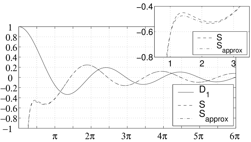
Figure 1: Plots of the correlation functions $D_{1}(X)$ and $S(X)$ which are responsible for spontaneous decay (”D”) and level shifts (”S”), respectively. $D_{1}$ becomes maximal at zero interatomic distance while $S$ tends to minus infinity there, due to Coulomb- and radiative self-energy of the atomic dipole. Both functions tend to zero as $X\rightarrow\infty$, expressing the fact that any kind of correlation must cease to exist for infinite distance. The inset shows a comparison between the exact shift function $S(X)$, based on eq. (23b), and the approximation $S_{\text{approx}}$, based on eq. (24), respectively.

where $\Gamma$ is the spontaneous emission rate of a single atom in a radiative vacuum. The argument of the function $D_{1}$ is equal to $2\pi$ times the distance $R_{AB}$ between atoms $A$ and $B$ measured in units of the wavelength $\lambda_{eg}=2\pi/k_{eg}$ of the Bohr transition $|e\rangle\rightarrow|g\rangle$. A plot of the function $X\mapsto D_{1}(X)$ is given in Fig. 1.

[Remark: In the more general case of arbitrarily aligned atoms there are two correlation functions $D_{1},D_{2}$ emerging in the decay matrix rather than just one. This is indicated by our denotation. For parallely aligned atoms, the contribution of $D_{2}$ vanishes.]

The level-shift matrix $\Delta_{AB}$ and the decay matrix $\Gamma_{AB}$ are connected by a dispersion relation which, for the case at hand, reads

$$\Delta_{AB}(E)=\frac{1}{2\pi}\int\limits_{0}^{\infty}dE^{\prime}\;\mathcal{P}\frac{\Gamma_{AB}(E_{G}+E^{\prime})}{E-E_{G}-E^{\prime}}\quad.$$ (22)

The energy $E_{G}=N\cdot E_{g}$ of the unperturbed joint atomic ground state will be negative in general. Using (22) the level shifts can be computed using appropriate complex contour integrals, with the result

$$\Delta_{AB}(E_{i}) =-\frac{1}{2}\Gamma\,S(X)\quad,\quad X=k_{eg}R_{AB}$$ (23a)

$$S(X) =\frac{3}{2}\left\{\frac{\cos X}{X}-\frac{\sin X}{X^{2}}-\frac{\cos X}{X^{3}}+\frac{1}{\pi X^{2}}\int\limits_{0}^{\infty}du\;\frac{e^{-u}\left(1+u+u^{2}\right)}{u^{2}+X^{2}}\right\}\quad.$$ (23b)

The integral on the right-hand side of (23b) can be approximated as follows: We replace the exponential $e^{-u}$ by $1$ for $0\leq u\leq 1$; and by $0$ for $u>1$. This leads to the following approximation for the function $S(X)$:

$$S(X)_{\text{approx}}\simeq\frac{3}{2}\left\{\frac{\cos X}{X}-\frac{\sin X}{X^{2}}-\frac{\cos X}{X^{3}}+\frac{1}{\pi X^{2}}\left[\frac{1-X^{2}}{X}\,\arctan\frac{1}{X}+1+\frac{1}{2}\,\ln\frac{1+X^{2}}{X^{2}}\right]\right\}\quad.$$ (24)

A plot of the exact function $S(X)$ as given in (23b), and its approximation (24), is given in Fig. 1.

The spatial dependence of the correlations between the atoms is now fully contained in the functions $D_{1}(X)$ (”decay”) and $S(X)$ (”shift”). Both functions tend to zero as $X\rightarrow\infty$; this is clear on physical grounds, since $X=\frac{2\pi|{\bf R}_{A}-{\bf R}_{B}|}{\lambda_{eg}}$ implies that the interatomic distance tends to infinity in this limit, in which case all correlations between the atoms must cease to exist. The only exception of course is the self-correlation of atom $A$, as expressed by the fact that the diagonal elements $\Gamma_{AA}$ are equal to one at each distance. Thus, the decay matrix $\Gamma_{AB}$ tends to $\Gamma\cdot\Eins$ as $X\rightarrow\infty$, implying that the spontaneous emission rate for any simply-excited collective state $\left|\mathcal{C}\right\rangle$ tends to the single-atom rate $\Gamma$, as expected.

Now we study the opposite limit: The decay matrix $\Gamma_{AB}$ has a well-defined limit for vanishing interatomic distance, since

$$\lim\limits_{X\rightarrow 0}D_{1}(X)=1\quad,$$ (25)

and as a consequence, $\Gamma_{AB}\rightarrow\Gamma\;\;\forall A,B$ in this limit. The reason for this behaviour is as follows: The limit $X\rightarrow 0$ defines the small-sample limit, in which all atomic dipoles are within each other’s near zone. It is easy to compute that, in this limit, their degree of correlation is proportional to the cosine ${\bf e}_{A}\bullet{\bf e}_{B}$, where $\mathbf{e}_{A}$ and $\mathbf{e}_{B}$ are unit vectors in the direction of the atomic dipoles. Thus, in the small-sample approximation, parallely aligned dipoles are maximally correlated while dipoles oriented perpendicularly are not correlated at all. In our sample, all dipoles are parallel, hence the limit (25).

On the other hand, the function $S(X)$ diverges in the limit $X\rightarrow 0$. The reason for this divergence is different depending on whether off-diagonal or diagonal elements of $\Delta_{AB}$ are considered. Let us first study the off-diagonal case:

Here, $R_{AB}\neq 0$, and we can rewrite (23a) in the form

$$\Delta_{AB}(E_{i})=\frac{d^{2}}{4\pi\epsilon_{0}\hbar}\frac{1}{R_{AB}^{3}}\;f(R_{AB})\quad,$$ (26)

where $f(R_{AB})$ is an analytic function of $R_{AB}$ which tends to $\frac{1}{2}$ as $R_{AB}$ tends to zero. This last result should be compared with the Coulomb dipole-dipole interaction between the two atoms $A$ and $B$,

$$V^{\text{dip}}_{AB}=\frac{\mathbf{d}_{A}\bullet\mathbf{d}_{B}-3\,\left(\mathbf{d}_{A}\bullet\mathbf{e}_{AB}\right)\left(\mathbf{d}_{B}\bullet\mathbf{e}_{AB}\right)}{4\pi\epsilon_{0}\,R_{AB}^{3}}\quad.$$ (27a)

For two classical dipoles which are parallel, $$\mathbf{d}_{A}\bullet\mathbf{d}_{B}=d^{2} \mathbf{e}_{AB} \mathbf{d}_{A}\bullet\mathbf{e}_{AB}=\mathbf{d}_{B}\bullet\mathbf{e}_{AB}=0$$, and which are aligned perpendicularly to their axis of connection, , (27a) takes the simpler form

$$V^{\text{dip}}_{AB}(R_{AB})=\frac{d^{2}}{4\pi\epsilon_{0}\,R_{AB}^{3}}\quad.$$ (27b)

It then follows that the level shifts in (26) contain the dipole-dipole Coulomb interaction between the charged ensembles $A$ and $B$, since (27b) is contained as a factor in the off-diagonal matrix element $\hbar\Delta_{AB}(E_{i})$ describing the level shift of the system due to the coupling to the radiative degrees of freedom as well as the dipole-dipole Coulomb interaction between atoms $A$ and $B$. So we could indeed write

$$\hbar\Delta_{AB}(E_{i})=V^{\text{dip}}_{AB}(R_{AB})\cdot f(R_{AB})\quad,$$ (28)

where $f$ now contains the effect of the purely radiative degrees of freedom. As mentioned above, in the limit $R_{AB}\rightarrow 0$ we have $f(R_{AB})\rightarrow\frac{1}{2}$; eq. (28) then implies that

$$\lim_{R_{AB}\rightarrow 0}\hbar\Delta_{AB}(E_{i})=\frac{1}{2}\lim_{R_{AB}\rightarrow 0}V^{\text{dip}}_{AB}(R_{AB})\quad,\quad A\neq B\quad.$$ (29)

We now turn to discuss the behaviour of the diagonal elements $\Delta_{AA}$: These quantities are infinite, since $R_{AA}=0$. This divergence remains even if only a single atom is considered, and has to do with the inevitable coupling of the atom to the longitudinal and transverse degrees of freedom of the radiation field. From (26 – 28) we learn that part of the divergence comes from the Coulomb dipole self-energy of atom $A$. The other contribution to the self-energy is associated with emission and reabsorption of virtual photons of the dipole which is an ongoing process even if only one atom is embedded in the vacuum. It emerges explicitly as a radiative dipole self-energy (an infinite $c$-number term), when the Göppert-Mayer transformation is performed on the Standard Hamiltonian. These processes are usually summarized by saying that the energy levels, together with the states, undergo radiative corrections.

As a consequence, the unperturbed states are not really the true physical states; rather, they are abstract constructions whose coupling to the continuum of radiation modes shifts their unperturbed energy by an infinite, but unobservable amount, an effect which is well-known in Quantum Field Theory Bjorken and Drell (1990a, b); Bogoliubov and Shirkov (1959); Itzykson and Zuber (1980); Ryder (1996); Bailin and Love (1986). This amount must be absorbed into the definition of the unperturbed energy, so that the energy of the initial state $\left|\psi_{t=0}\right\rangle=\left|\mathcal{C}\right\rangle$ becomes renormalized

$$E_{i} \longrightarrow E_{i}+\lim\limits_{X\rightarrow 0}\hbar\Delta_{AA}(E_{i})\equiv\widetilde{E}_{i}\quad,$$ (30)

where $\widetilde{E}_{i}$ is now assumed to have a finite value, namely the value unperturbed by the presence of $N-1$ other atoms; as a consequence, $E_{i}$ must be assumed to have been infinite in the first place. In turn, we now must subtract the same infinite quantity from the diagonal elements of the level-shift matrix, which amounts to a redefinition

$$\Delta_{AB}(E_{i})\longrightarrow\widetilde{\Delta}_{AB}(E_{i})\equiv\begin{cases}\quad\Delta_{AB}(E_{i})&,\quad A\neq B\;,\\ \quad 0&,\quad A=B\;.\end{cases}$$ (31)

As a consequence, the only observable level-shifts are now those due to interatomic interactions.

Using the functions $D_{1}$ and $S$, the matrix element (20a) can be written as

$$\left\langle A,0\right|\mathcal{H}(E_{i})\left|B,0\right\rangle=\left\{\begin{array}[]{c@{}cl@{}c}-\frac{\hbar\Gamma}{2}\,\bigg{[}\,S(k_{eg}R_{AB})+i\,D_{1}(k_{eg}R_{AB})\,\bigg{]}&\;,&A\neq B&\;,\\[10.0pt] \widetilde{E}_{i}-i\,\frac{\hbar\Gamma}{2}&\;,&A=B&\;.\end{array}\right\}=\widetilde{E}_{i}\,\delta_{AB}-\frac{\hbar\Gamma}{2}\,\mathcal{R}_{AB}\quad,$$ (34)

where the matrix elements $\mathcal{R}_{AB}$ are determined by the function $M(X)=S(X)+iD_{1}(X)$, which can be determined from (21c) and (24) to be

$$M(X)\equiv S(X)+i\,D_{1}(X)\simeq\frac{3}{2}\,e^{iX}\,\left(\frac{1}{X}+\frac{i}{X^{2}}-\frac{1}{X^{3}}\right)+\frac{3}{2\pi X^{2}}\left(\frac{1-X^{2}}{X}\,\arctan\frac{1}{X}+1+\frac{1}{2}\,\ln\frac{1+X^{2}}{X^{2}}\right)\quad.$$ (35)

Evidently, if we have found the left/right eigenvectors of $\mathcal{R}$, then we have diagonalized the whole channel Hamiltonian, for $\mu_{p}$ is an eigenvalue of $\mathcal{R}$ if and only if $\widetilde{E}_{i}-\frac{\hbar\Gamma}{2}\,\mu_{p}$ is an eigenvalue of $\widetilde{E}_{i}\,\Eins_{N}-\frac{\hbar\Gamma}{2}\,\mathcal{R}$. It follows from eq. (11) that the matrix of the channel Hamiltonian $\mathcal{H}(E_{i})$ in the basis $\left|A,0\right\rangle$ can be written as

$$\left\langle A,0\right|\mathcal{H}(E_{i})\left|B,0\right\rangle=\sum_{p=1}^{N}\left\langle A,0\right|\left.\mathcal{C}_{p}\right\rangle\bigg{\{}\widetilde{E}_{i}-\frac{\hbar\Gamma(k_{eg})}{2}\,\mu_{p}\bigg{\}}\left\langle\mathcal{C}_{p}^{*}\right|\left.B,0\right\rangle\quad.$$ (36)

We must be aware that $\widetilde{E}_{i}$ has been renormalized by an infinite amount and is now to be regarded as the finite, physically meaningful energy of the simply-excited atomic sample when all interatomic distances are infinite. A comparison of (36) with (20a) now shows that the quantities $-\frac{\hbar\Gamma}{2}\mu_{p}$ are the right eigenvalues of the matrix

$$\hbar\widetilde{\Delta}_{AB}(E_{i})-i\frac{\hbar}{2}\Gamma_{AB}(E_{i})\quad.$$ (37)

It is therefore appropriate to denote the real and imaginary parts of these eigenvalues according to

$$-\frac{\hbar\Gamma}{2}\bigg{(}\mathfrak{Re}\!~{}\mu_{p}+i\mathfrak{Im}\!~{}\mu_{p}\bigg{)}=\hbar\widetilde{\Delta}_{p}-i\frac{\hbar}{2}\Gamma_{p}\quad,$$ (38)

and hence

$$\widetilde{\Delta}_{p} =-\frac{\Gamma}{2}\;\mathfrak{Re}\!~{}\mu_{p}\quad,$$ (39a)

$$\Gamma_{p} =\hskip 7.22212pt\Gamma\;\mathfrak{Im}\!~{}\mu_{p}\quad,$$ (39b)

where $\widetilde{\Delta}_{a}$ now denotes the renormalized level-shifts. A comparison of (36) with (11), on the other hand, shows that the quantities in curly brackets in (36) are equal to $\Lambda_{p}$. From (36, 37, 38) it then follows that $\Lambda_{p}$ should be decomposed according to

$$\Lambda_{p}=\,\widetilde{E}_{i}+\hbar\widetilde{\Delta}_{p}-i\frac{\hbar}{2}\Gamma_{p}\quad,\quad\Gamma_{p}>0\quad,$$ (40)

where all imaginary parts $\Gamma_{p}$ must be positive due to (17).

We now insert (40) into equation (18) for the transition amplitude and compute our target quantity, namely the probability $P(t)$ for the atomic sample at time $t>0$ to be found in the radiationless $Q$-space, as defined in (6); the result is

$$P(t) =\sum_{B_{1},B_{2}}c^{*}_{B_{2}}\;P_{B_{2}B_{1}}\;c_{B_{1}}\quad,$$ (41a)

$$P_{B_{2}B_{1}} =\sum_{A,p_{1},p_{2}=1}^{N}\left\langle B_{2},0\right|\left.\mathcal{C}_{p_{2}}^{*}\right\rangle\left\langle\mathcal{C}_{p_{2}}\right|\left.A,0\right\rangle\;e^{i\left(\widetilde{\Delta}_{p_{2}}-\widetilde{\Delta}_{p_{1}}\right)t}$$

$$\times e^{-\frac{1}{2}\left(\Gamma_{p_{1}}+\Gamma_{p_{2}}\right)t}\;\left\langle A,0\right|\left.\mathcal{C}_{p_{1}}\right\rangle\left\langle\mathcal{C}_{p_{1}}^{*}\right|\left.B_{1},0\right\rangle\quad.$$ (41b)

For the given radius $r$, number of atoms $N$, and configuration (a) or (b), let $\Lambda_{{\text{min}}}$ be the eigenvalue with the smallest decay rate,

$$\Gamma_{{\text{min}}}\leq\Gamma_{p}\quad\text{for all $p=1,\ldots,N$}\quad.$$ (42)

Then the associated correlated state

$$\left|\mathcal{C}\right\rangle=\frac{1}{\sqrt{\left\langle\mathcal{C}_{{\text{min}}}|\mathcal{C}_{{\text{min}}}\right\rangle}}\,\left|\mathcal{C}_{{\text{min}}}\right\rangle\quad$$ (43)

has the longest lifetime with respect to spontaneous decay [saying nothing about stability against environmental perturbations], and hence is a candidate for a single-photon trap.

IV Cyclic symmetry of the circular atomic configurations

In the remaining part of this paper we shall apply the above theory mainly to circular configurations of atoms, containing $N$ atoms along the perimeter of the circle, and an optional atom at the center. The system with [without] central atom is referred to respectively as configuration a) [ b)], see Fig. 2. In the last section we briefly give some results about configuration c), involving $N$ atoms arranged along a straight line.

Now let us study the circular configurations: We shall construct the eigenvectors $\left|\mathcal{C}_{p}\right\rangle$ of $\mathcal{H}(\widetilde{E}_{i})$ explicitly by group-theoretical means, taking advantage of the fact that the system has a cyclic symmetry group

$$G=\left\{e,T,T^{2},\ldots,T^{N-1}\right\}\quad,\quad T^{N}=e\quad,$$ (44)

where the generator $T$ is realized by a (passive) rotation at the angle $2\pi/N$ about the symmetry axis of the circle, and $N$ is the number of outer atoms along the perimeter of the circle. This holds for both configurations a) and b). All cyclic groups of the same order $N$ are isomorphic to the group of integers $\mathbb{Z}_{N}=\{0,1,\ldots,N-1\}$ with group operation $A\circ B=A+B\mod N$, unit element $0$, and inverses $A^{-1}=-A\mod N$. The set of all unitary irreducible representations of $\mathbb{Z}_{N}$ is given by

$$\Gamma^{p}\left(T^{A}\right)=\exp\left(\frac{2\pi ipA}{N}\right)\quad,\quad A=1,2,\ldots,N\quad,$$ (45)

where $p=0,1,\ldots,N-1$. The atoms are located at the center and along the perimeter of a circle with radius $r$ such that

$$\mathbf{R}_{z} =(0,0)\quad,$$ (46)

$$\mathbf{R}_{A} =r\,\left(\cos\frac{2\pi(A-1)}{N},\,\sin\frac{2\pi(A-1)}{N}\right)\quad,$$

for $A=1,\ldots,N$.

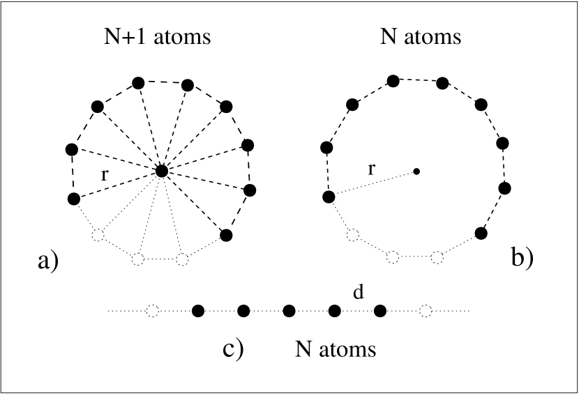
Figure 2: The configurations of $N(+1)$ atoms which are examined: In configuration (a), $N$ outer atoms form a regular $N$-polygon with radius $r$, plus an atom at the center. Configuration (b) is the same as a), but without the central element. Configuration (c) has $N$ atoms in a linear chain with next-neighbour distance $d$.

As mentioned above, the basic symmetry operation in our system is the shift $T$, corresponding to a passive rotation $T_{c}$ about the symmetry axis by an angle $2\pi/N$. $T_{c}$ transforms the coordinates $\mathbf{R}_{A}$ of the outer atoms and the central atom $\mathbf{R}_{z}$ according to

$$T_{c}\,\mathbf{R}_{A} =\mathbf{R}_{A-1}\quad,\quad N+1=1\mod N\quad,$$ (47)

$$T_{c}\,\mathbf{R}_{z} =\mathbf{R}_{z}\quad.$$

Here $\mathbf{R}$ denotes the triple of coordinates with respect to an orthonormal basis which undergoes rotation, and not the invariant vector. Next we need to construct the action of the unitary operator $T$ associated with the coordinate transformation $T_{c}$ given in (47) on the state vectors of the system. $T$ operates on the atomic degrees of freedom only, so we can ignore the photon states for the time being. It is sufficient to specify the action of $T$ on product states; superscripts denote the label of the atoms:

$$T\,\left|\psi^{z}_{i_{z}}\right\rangle\otimes\left|\psi^{1}_{i_{1}}\right\rangle\otimes\cdots\otimes\left|\psi^{N}_{i_{N}}\right\rangle=\left|\psi^{z}_{i_{z}}\right\rangle\otimes\left|\psi^{1}_{i_{2}}\right\rangle\otimes\cdots\otimes\left|\psi^{N-1}_{i_{N}}\right\rangle\otimes\left|\psi^{N}_{i_{1}}\right\rangle\quad.$$ (48)

This action derives from eq. (47), and preserves the subspaces of any given degree of excitation. On the single-excitation subspace, $T$ acts according to

$$T\,\left|A\right\rangle=\left|A-1\right\rangle\quad,\quad T\,\left|z\right\rangle=\left|z\right\rangle\quad,$$ (49)

and hence has the matrix elements

$$T_{AB}=\left\langle A\right|T\left|B\right\rangle=\delta_{A,B-1}\quad.$$ (50)

The inverse is given by the transposed matrix, $T^{-1}=T^{T}$, expressing the fact that $T$ is a unitary operator.

Eqs. (49) are consistent with the transformation behaviour of a scalar wave function: Suppose that $\psi(\mathbf{x})=\left\langle\mathbf{x}|\psi\right\rangle$ is a wave function in the coordinate system $\mathbf{x}$, and $T_{c}\mathbf{x}=\mathbf{x}^{\prime}$ is a coordinate transformation. The wave function is a scalar under the associated unitary transformation $T$ on the state space if, in the new coordinates $\mathbf{x}^{\prime}$, the new state vector $|\psi^{\prime}\rangle$ with wave function $\psi^{\prime}(\mathbf{x}^{\prime})=\langle T_{c}\mathbf{x}|T\psi\rangle$ satisfies

$$\psi^{\prime}(\mathbf{x}^{\prime}) =\psi(\mathbf{x})\quad,$$ (51a)

and as a consequence

$$T\,\left|\mathbf{x}\right\rangle =\left|T_{c}\,\mathbf{x}\right\rangle\quad.$$ (51b)

This should be compared with the case of the simply-excited correlated states at hand: Here we can consider the sites $\mathbf{R}_{z},\mathbf{R}_{A}$ of the atoms as discrete locations analogous to the parameters $\mathbf{x}$ in (51b). The simply-excited state $\left|\mathcal{C}\right\rangle$ may be regarded as describing a scalar quasi-particle (a Frenkel exciton) for which the states $|z\rangle,|A\rangle$ are the analogues of the state vectors $|\mathbf{x}\rangle$ for an ordinary spinless particle. The transformations (47) then imply (49), in full analogy to (51b).

The channel Hamiltonians of both configurations are invariant under this transformation,

$$T^{-1}\,\mathcal{H}\,T=\mathcal{H}\quad,\quad T^{-1}\,\mathcal{R}\,T=\mathcal{R}\quad,$$ (52)

where the matrix $\mathcal{R}$ was defined in eq. (34). Relations (52) can be proven as follows: The matrix $\mathcal{R}$ is symmetric by construction, and, for configuration (a), has components

$$\mathcal{R}=\left(\begin{array}[]{c|cccc}i&\mathcal{R}_{z1}&\mathcal{R}_{z2}&\cdots&\mathcal{R}_{zN}\\ \hline\cr\mathcal{R}_{1z}&i&\mathcal{R}_{12}&\cdots&\mathcal{R}_{1N}\\ \mathcal{R}_{2z}&\mathcal{R}_{21}&i&&\vdots\\ \vdots&\vdots&&\ddots&\vdots\\ \mathcal{R}_{Nz}&\mathcal{R}_{N1}&\mathcal{R}_{N2}&\cdots&i\end{array}\right)\quad$$ (53)

such that

$$\mathcal{R}_{z1} =\mathcal{R}_{z2}=\cdots=\mathcal{R}_{zN}\quad,$$ (54a)

$$\mathcal{R}_{A,B} =\mathcal{R}_{A+C,B+C}\quad\text{for}\quad 1\leq A,B\leq N\quad,$$ (54b)

where in (54b) all indices are to be taken modulo $N$. The relations (54), in turn, follow from the fact that

$$R_{z1} =R_{z2}=\cdots=R_{zN}=r\quad,$$ (55a)

$$R_{AB} =R_{A+C,B+C}\quad\text{for}\quad 1\leq A,B\leq N\quad,$$ (55b)

and arbitrary $C$, where $r$ is the radius of the circle. If the matrix representation (50) of the operator $T$ is used on (53) we obtain (52). Similarly, for the configuration (b) without central atom, the relevant operators are given by the lower right block matrices in eqs. (50) and (53), so that again (52) holds. Thus, we have proven that the generator $T$ of the cyclic group $\mathbb{Z}_{N}$ commutes with the matrix $\mathcal{R}$, and hence with the (non-Hermitean) channel Hamiltonian $\mathcal{H}(E_{i})$, at least on the single-excitation subspace; but these arguments can easily be extended to show that $T$ and $\mathcal{H}$ commute on all subspaces. Hence we have

$$\Big{[}\,T,\,\mathcal{R}\,\Big{]}=0\quad,\quad\Big{[}\,T,\,\mathcal{H}\,\Big{]}=0\quad.$$ (56)

Just as in the case of Hermitean operators, the commutativity (56) implies the existence of a common system of eigenvectors of $\mathcal{H}$ and $T$: Suppose that $v$ is an eigenvector of $T$, regarded as a complex column vector of dimension $N$ or $(N+1)$, with eigenvalue $t$, so that $Tv=tv$. Then

$$T\Big{(}\mathcal{H}v\Big{)}=t\Big{(}\mathcal{H}v\Big{)}\quad,$$ (57)

where we have used (56). Eq. (57) says that $\mathcal{H}$ preserves all eigenspaces of $T$, i.e. if $\mathsf{T}(t)$ is the subspace corresponding to the eigenvalue $t$, then

$$\mathcal{H}\,\mathsf{T}(t)\subset\mathsf{T}(t)\quad.$$ (58)

On the other hand we must have $T^{A}v=t^{A}v$, and in particular

$$v=\Eins\,v=T^{N}\,v=t^{N}\,v\quad,$$ (59)

from which it follows that

$$t=\exp\left(\frac{2\pi ip}{N}\right)=\Gamma^{p}(T)\quad$$ (60)

for some $p\in\{0,1,\ldots,N-1\}$, and we see that the eigenvalues of $T$ are just the one-dimensional matrices $\Gamma^{p}$, eq. (45), of the irreducible representations of the cyclic group $\mathbb{Z}_{N}$. Accordingly, we can label the eigenspaces of $T$ by the index $p$ of the representation as $\mathsf{T}(t)\equiv\mathsf{T}_{p}$.

We see that the eigenvectors $v$ of $T$ in the state space of the atomic system satisfy $T\,v=\Gamma^{p}(T)\,v$ and therefore span carrier spaces for the irreducible representations (45) of the symmetry group. Since $T$ is unitary, these carrier spaces are orthogonal, and their direct sum is the total atomic state space. Since the channel Hamiltonian $\mathcal{H}$ preserves the eigenspaces $\mathsf{T}_{p}$ of $T$ according to (58) we see that a method to simplify the diagonalization of $\mathcal{H}$ is given as follows:

1. We first determine the eigenspaces $\mathsf{T}_{p}$ of $T$ on the state space of the atomic degrees of freedom. These eigenspaces are comprised by vectors $v$ each of which transforms as a basis vector for a definite irreducible representation $\Gamma^{p}(T)$ of the symmetry group $\mathbb{Z}_{N}$,

   $$T\,v=\Gamma^{p}(T)\,v\quad\text{for all $v\in\mathsf{T}_{p}$}\quad.$$ (61)

2. The channel Hamiltonian $\mathcal{H}$ preserves each eigenspace $\mathsf{T}_{p}$, so that we can diagonalize $\mathcal{H}$ on each $\mathsf{T}_{p}$ separately.

Since the eigenspaces $\mathsf{T}_{p}$ are smaller in dimension than the original state space we can expect a significant simplification of the diagonalization procedure for $\mathcal{H}$. This will be explicitly demonstrated in the following sections.

V Eigenspaces of the generator $T$ of the symmetry group

We now construct the eigenspaces $\mathsf{T}_{p}$ of $T$ on the single-excitation subspaces of the atomic systems with and without a central atom. These eigenspaces may be constructed by a standard procedure Cornwell (1984) by writing down the projection operators $\mathcal{P}^{p}$ onto $\mathsf{T}_{p}$ on the state space of atomic degrees of freedom. These projectors have the following property: Given an arbitrary element $|\mathcal{C}\rangle$ of the (single-excitation) state space, its image $\mathcal{P}^{p}|\mathcal{C}\rangle$ transforms like a basis vector for the one-dimensional unitary irreducible representation $\Gamma^{p}(T)$ defined in (45),

$$T^{A}\,\Big{(}\mathcal{P}^{p}\left|\mathcal{C}\right\rangle\Big{)}=\Gamma^{p}\left(T^{A}\right)\,\Big{(}\mathcal{P}^{p}\left|\mathcal{C}\right\rangle\Big{)}=\exp\left(\frac{2\pi ipA}{N}\right)\,\Big{(}\mathcal{P}^{p}\left|\mathcal{C}\right\rangle\Big{)}\quad.$$ (62)

For the cyclic group $\mathbb{Z}_{N}$ at hand, the projectors are defined by Cornwell (1984)

$$\mathcal{P}^{p}=\frac{1}{N}\sum_{A=0}^{N-1}\Gamma^{p}\left(T^{A}\right)^{*}\,T^{A}=\frac{1}{N}\sum_{A=0}^{N-1}\exp\left(-\frac{2\pi ipA}{N}\right)\,T^{A}\quad,$$ (63a)

where the action of $$T p 0 (N-1) T \mathcal{P}^{p}$$ was defined in (49). In (63a), ranges between and and covers all irreducible representations. The fact that is unitary implies that the are Hermitean and have the projector property

$$\mathcal{P}^{p}\mathcal{P}^{q}=\delta_{pq}\,\mathcal{P}^{p}\quad.$$ (63b)

The sum over all $$\mathcal{P}^{p}$$ gives the identity on the atomic state space,

$$\sum_{p=0}^{N-1}\mathcal{P}^{p}=\Eins\quad.$$ (63c)

The completeness relation (63c) implies that the state space of the atomic system may be spanned by a basis such that each of its members transforms as a basis vector (62) of an irreducible multiplet (In the present case, all multiplets are singlets, since all $\Gamma^{p}$ are one-dimensional).

We now construct such a basis in the single-excitation subspace of the atomic state space which has dimension $(N+1)$ for configuration (a) and $N$ for configuration (b). We first treat case (a): We start with an arbitrary correlated state $\left|\mathcal{C}\right\rangle$,

$$\left|\mathcal{C}\right\rangle=c_{z}|z,0\rangle+\sum_{A=1}^{N}c_{A}|A,0\rangle\quad,$$ (64)

and apply the projector $\mathcal{P}^{p}$; the result is

$$\mathcal{P}^{p}\,\left|\mathcal{C}\right\rangle=\left\{\frac{1}{N}\sum_{A=0}^{N-1}\exp\left(-\frac{2\pi ipA}{N}\right)\right\}\,c_{z}\,\left|z,0\right\rangle+\left\{\frac{1}{N}\sum_{B=1}^{N}\exp\left(-\frac{2\pi ipB}{N}\right)\,c_{B}\right\}\;\times\sum_{A=1}^{N}\exp\left(\frac{2\pi ipA}{N}\right)\,\left|A,0\right\rangle\quad.$$ (65)

The factor before $c_{z}$ is equal to $\delta_{p0}$; thus we see that the general form of a normalized basis vector carrying the irreducible representation $\Gamma^{p}$ is

$$\mathcal{P}^{p}\left|\mathcal{C}\right\rangle=\delta_{p0}\,c_{z}\,\left|z,0\right\rangle+c\sum_{A=1}^{N}\exp\left(\frac{2\pi ipA}{N}\right)\,\left|A,0\right\rangle\quad,\quad|c_{z}|^{2}+|c|^{2}=1\quad.$$ (66)

It follows that, for $p\neq 0$, the eigenspaces of $T$ are one-dimensional, and are spanned by basis vectors

$$\left|\mathcal{C}_{p}\right\rangle\equiv\frac{1}{\sqrt{N}}\sum_{A=1}^{N}\exp\left(\frac{2\pi ipA}{N}\right)\,\left|A,0\right\rangle\quad,\quad\langle\mathcal{C}_{p}|\mathcal{C}_{p}\rangle=1\quad.$$ (67)

This statement is true for both configurations (a) and (b). We emphasize again that, here, $N$ denotes the number of outer atoms. The coefficients $c^{p}_{A}=\left\langle A,0|\mathcal{C}_{p}\right\rangle$ of states (67) have the property that

$$c_{A}^{N-p}=\left(c_{A}^{p}\right)^{*}\quad.$$ (68)

In Fig. 3 we plot the real parts of $c^{p}_{A}$ for some of the $p$-states with $N=50$ and $N=51$ outer atoms.

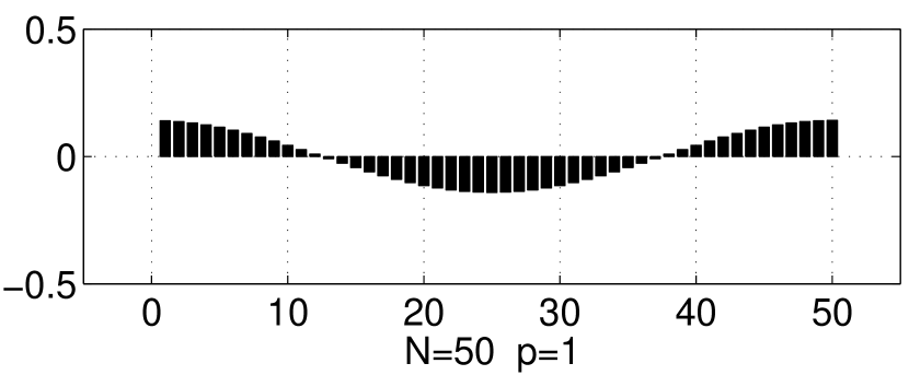
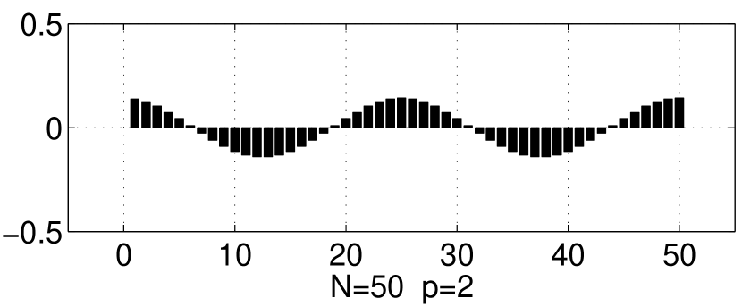
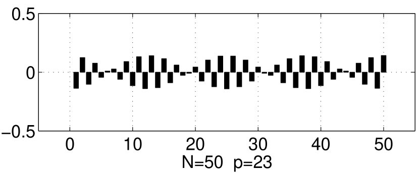
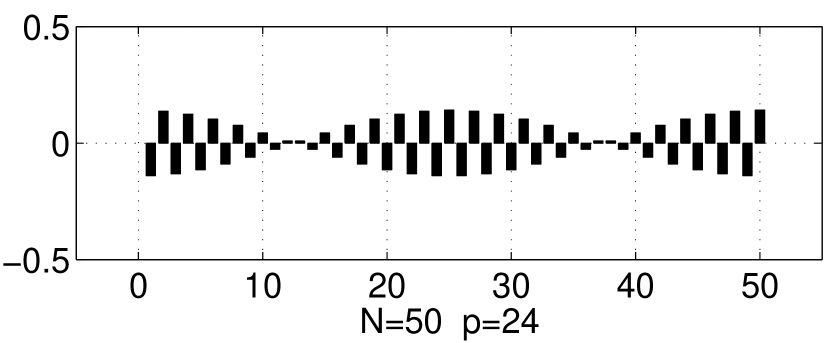
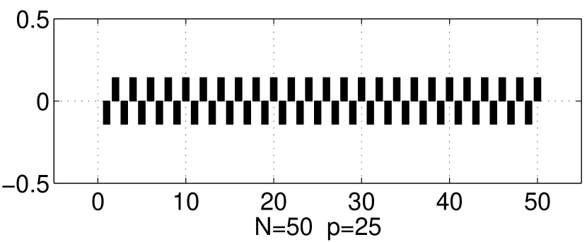
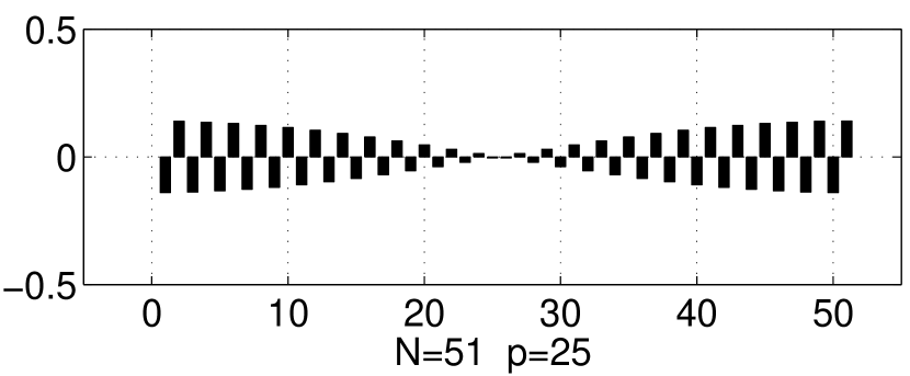
Figure 3: The real parts $\mathfrak{Re}\!~{}c^{p}_{A}$ of the coefficients $c^{p}_{A}=\left\langle A,0|\mathcal{C}_{p}\right\rangle$ for the eigenstates $p=1,2,23,24,25$ of a configuration with $N=50$ outer atoms, and for $p=25$ with $N=51$ outer atoms. Since $p\neq 0$, these coefficients are the same for both configurations (a) and (b).

If $p=0$, the associated eigenspace $\mathsf{T}_{0}$ is one-dimensional for configuration (b), and is spanned by

$$\left|\mathcal{C}_{0}\right\rangle\equiv\frac{1}{\sqrt{N}}\sum_{A=1}^{N}\left|A,0\right\rangle\quad.$$ (69)

For configuration (a), the eigenspace $\mathsf{T}_{0}$ is two-dimensional, with basis vectors $\left|\mathcal{C}_{0}\right\rangle$ as in (69) and a second basis vector

$$\left|\mathcal{C}_{z}\right\rangle\equiv\left|z,0\right\rangle\quad.$$ (70)

On account of (63b), basis vectors pertaining to different irreducible representations are automatically orthogonal. For the case of the two-dimensional $p=0$ subspace of configuration (a) the two basis elements may always be chosen as orthonormal, as we have done in (69, 70).

Thus we have accomplished the decomposition of the space of atomic degrees of freedom into carrier spaces $\mathsf{T}_{p}$ for the irreducible representations $\Gamma^{p}$ of the symmetry group $\mathbb{Z}_{N}$ for both configurations (a) and (b). All that remains to be done now is to diagonalize the channel Hamiltonian $\mathcal{H}$ on each of these subspaces separately.

VI Diagonalization of the channel Hamiltonian on carrier spaces of the symmetry group

VI.1 Configuration (b)

We first discuss configuration (b) without central atom. In this case, each of the eigenspaces of $T$ is one-dimensional, and is spanned by states (67, 69). Since $\mathcal{H}$ commutes with $T$, it follows that each of the $\left|\mathcal{C}_{p}\right\rangle$, $p=0,\ldots,N-1$, is automatically a right eigenvector of $\mathcal{H}$, or equivalently, of the matrix $\mathcal{R}$. The associated eigenvalue is found to be

$$\mu_{p}=i+\sum_{A=2}^{N}M(k_{eg}R_{1A})\,\cos\left({\frac{2\pi ip(A-1)}{N}}\right)\quad,$$ (71)

which shows that

$$\mu_{N-p}=\mu_{p}\quad,$$ (72)

hence some of the eigenvalues are degenerate; the exact result is presented in Table 1.

Level degeneracy for configurations (a) and (b)

$$\begin{array}[]{| @{\hspace{.5em}} r @{\hspace{.5em}} || @{\hspace{.5em}} r@{}c@{}l @{\hspace{.1em}} @{\hspace{.5em}} | @{\hspace{.5em}} r@{}c@{}l @{\hspace{.5em}} |}\hline\cr\hskip 5.0pt\lx@intercol\hfil\hskip 5.0pt\vrule\vrule\hskip 5.0pt&N&=&2n+1\hfil\hskip 1.00006pt\hskip 5.0pt\vrule\hskip 5.0pt&N&=&2n\hfil\hskip 5.0pt\\ \hline\cr\hline\cr\hskip 5.0pt\lx@intercol\hfil\text{degenerate}\hskip 5.0pt\vrule\vrule\hskip 5.0pt&p&=&\begin{array}[]{r@{}c@{}l}1,&\ldots,&n\\ 2n,&\ldots,&n+1\end{array}\hfil\hskip 1.00006pt\hskip 5.0pt\vrule\hskip 5.0pt&p&=&\begin{array}[]{r@{}c@{}l}1,&\ldots,&n-1\\ 2n-1,&\ldots,&n+1\end{array}\hfil\hskip 5.0pt\\ \hline\cr\hskip 5.0pt\lx@intercol\hfil\text{non-degenerate}\hskip 5.0pt\vrule\vrule\hskip 5.0pt&p&=&0\,(\pm)\hfil\hskip 1.00006pt\hskip 5.0pt\vrule\hskip 5.0pt&p&=&0\,(\pm),n\hfil\hskip 5.0pt\\ \hline\cr\end{array}$$

Table 1: Degeneracy of the eigenvalues for quantum numbers $p=0(\pm),\ldots,N-1$, for odd and even $N$, for configurations (a) and (b). Vertically stacked $p$ values in the second row are mutually degenerate.

On making use of (35) we finally find

$$\mu_{p}=\sum_{A=2}^{N}S(k_{eg}R_{1A})\,\cos\left(\frac{2\pi p(A-1)}{N}\right)+i\Bigg{\{}1+\sum_{A=2}^{N}D_{1}(k_{eg}R_{1A})\,\cos\left(\frac{2\pi p(A-1)}{N}\right)\Bigg{\}}\quad,$$ (73)

where the real/imaginary parts contains the level shifts and decay rates, respectively. A plot of these quantities for the first four eigenvalues for $N=7$ outer atoms is given in Fig. 4, where the approximated shift function $S_{\text{approx}}$ based on eq. (24) has been used.

VI.2 Mechanisms for super- and subradiance

The Figures 3 and 4 give some insight into the mechanism of super- and subradiance. Studying first the limit of vanishing radius $r\rightarrow 0$, hence vanishing interatomic distance, we see in Fig. 4 that the $p=0$ state is the only one which has a nonvanishing decay rate in this limit: All atomic dipoles are aligned parallely in this state [see eq. (69)], and vanishing distance on a length scale of wavelength means that all radiation emitted coherently from the sample must interfere completely constructively. Hence, the sample radiates faster than a single atom by a factor $N$, since the decay rate is

$$\lim\limits_{r\rightarrow 0}\Gamma_{p=0}=N\cdot\Gamma\quad,$$ (74)

as follows from eqs. (73) and (25). Conversely, the suppression of spontaneous decay for the states with $p>0$ is a consequence of the fact that the dipoles have alternating orientations, see eq. (67) and Fig. 3, so that, in the small-sample limit $r\rightarrow 0$, roughly one-half of the atoms radiate in phase, while the other half has a phase difference of $\pi$; hence

$$\lim\limits_{r\rightarrow 0}\Gamma_{p>0}=0\quad.$$ (75)

This behaviour is exemplified by the plots of $\Gamma_{1},\Gamma_{2},\Gamma_{3}$ in Fig. 4. However, the destructive interference in the $(p>0)$ states is independent of how adjacent dipoles are oriented. For example, in the limit $r\ll\lambda$, the decay rate should not be noticeably affected by rearranging the dipoles in different patterns as long as the 50:50 ratio of parallel-antiparallel dipoles is kept fixed. What will be affected by such a redistribution is the level shift, since the Coulomb interaction between the dipoles in the sample may change towards more attraction or repulsion between the atoms. By this mechanism we can explain the divergent behaviour of the level shifts in the small-sample limit: The shift of the $p=0$ state always behaves like

$$\lim\limits_{r\rightarrow 0}\Delta_{p=0}=+\infty\quad,$$ (76)

which arises from the Coulomb repulsion of the parallely aligned dipoles. On the other hand, the level shifts for the $(p>0)$ states depend on the relative number of parallely aligned dipoles in the immediate neighbourhood of a given dipole, or conversely, on the degree of balancing the Coulomb repulsion by optimal pairing of antiparallel dipoles. As a consequence, states for which $p$ is close to zero always have positive level shifts, since the Coulomb repulsion between adjacent dipoles is badly balanced, as seen in the first two plots in Fig. 3, and the behaviour of $\Delta_{0},\Delta_{1}$ in Fig. 4. On the other hand, states for which $p$ is close to $N/2$ tend to have antiparallel orientation between adjacent dipoles, hence the Coulomb interaction is now largely attractive, which explains why these states have negative level shifts in the limit $r\ll\lambda$. This is seen in the last four plots in Fig. 3 and the behaviour of $\Delta_{2},\Delta_{3}$ in Fig. 4.

The same mechanism clearly also governs the super- or subradiance of the sample with finite interatomic distance. In this case the information about the orientation of surrounding dipoles at sites $\mathbf{R}_{A}$ is contained in the transverse electric field, which arrives at the site $\mathbf{R}_{1}$ with a retardation $|\mathbf{R}_{A}-\mathbf{R}_{1}|/c$. Thus, in addition to the phase difference imparted by the coefficients $c^{p}_{A}$, there is another contribution to the phase from the spatial retardation, which accounts for the dependence of the level shifts and decay rates on the radius $r$. Apart from this additional complication, the physical mechanism determining whether a given state is super- or subradiant is clearly the same as in the small-sample limit, and can be traced back to the mutual interference of the radiation emitted by each atom, arriving at a given site $\mathbf{R}_{1}$. This radiation is emitted coherently by the atoms on account of the fact that the sample occupies a pure collective state.

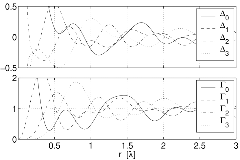
Figure 4: Relative level shifts $\widetilde{\Delta}_{p}/\Gamma$ and decay rates $\Gamma_{p}/\Gamma$ for the states $p=0,1,2,3$ with $N=7$ outer atoms and no central atom. From the second plot we see that none of the $p$-states can generally be declared as super- or subradiant; rather, for each state there exist ranges of the radius $r$ for which the state $\left|\mathcal{C}_{p}\right\rangle$ is maximally super- or maximally subradiant. The physical reason for this dependence lies in the interference due to varying phase differences between spatially retarded radiative contributions from all but one atom, at the site of a given atom.

VI.3 Configuration (a)

Now we turn to compute the complex energy eigenvalues and eigenvectors for configuration (a) with central atom. For $p=1,\ldots,N-1$, the basis vectors carrying irreducible representations of the symmetry group are the same as before, and are given in eq. (67). Consequently, they are also right eigenvectors of the matrix $\mathcal{R}$. The associated eigenvalues $\mu_{p}$ turn out to be the same as for configuration (b) and thus are given by formulae (71, 73). This result means that the presence or absence of the central atom makes no difference if the system occupies one of the modes $\left|\mathcal{C}_{p}\right\rangle$, $p=1,\ldots,N-1$, since the central atom is not occupied in the states (67).

On the other hand, the eigenspace $\mathsf{T}_{0}$ of $T$ corresponding to the $p=0$ representation is now two-dimensional and is spanned by $\Gamma^{0}$-basis vectors (69) and (70). Since $\mathsf{T}_{0}$ is preserved by $\mathcal{H}(\widetilde{E}_{i})$, we now need to diagonalize the channel Hamiltonian in this subspace: The representation of the matrix $\mathcal{R}$ in the basis $\left|\mathcal{C}_{0}\right\rangle,\left|\mathcal{C}_{z}\right\rangle$ is

$$\mathcal{R}^{\prime}=\Big{[}\mathcal{R}\Big{]}_{\left|\mathcal{C}_{0}\right\rangle,\left|\mathcal{C}_{z}\right\rangle}=\left(\begin{array}[]{c|c}\sum_{A=1}^{N}\mathcal{R}_{1A}&\sqrt{N}\,\mathcal{R}_{1z}\\[8.0pt] \hline\cr\rule{0.0pt}{15.0pt}\sqrt{N}\,\mathcal{R}_{1z}&i\end{array}\right)\quad.$$ (77)

Thus, we must diagonalize a non-Hermitean matrix of the form $\mathcal{R}^{\prime}=\left(\begin{array}[]{cc}a&b\\ b&i\end{array}\right)$. The diagonalization yields $\mathcal{R}^{\prime}\,\left|\mathcal{C}_{0,\pm}\right)=\mu_{0\pm}\,\left|\mathcal{C}_{0,\pm}\right)$, where temporarily we have defined

$$\mu_{0\pm}=\frac{a+i}{2}\pm\frac{1}{2}\sqrt{(a-i)^{2}+4b^{2}}\quad,$$ (78)

and

$$\left|\mathcal{C}_{0+}\right)=\bigg{(}\,\frac{1}{\sqrt{1+c^{2}}}\,,\;\frac{c}{\sqrt{1+c^{2}}}\,\bigg{)}^{T}\quad,\quad\left|\mathcal{C}_{0-}\right)=\bigg{(}\,-\frac{c}{\sqrt{1+c^{2}}}\,,\;\frac{1}{\sqrt{1+c^{2}}}\,\bigg{)}^{T}\quad,$$ (79a)

$$c=\frac{2b}{a-i+\sqrt{(a-i)^{2}+4b^{2}}}\quad.$$ (79b)

These definitions will undergo some refinement, as we shall explain below. The eigenvectors $\left|\mathcal{C}_{0\pm}\right\rangle$ corresponding to the column vectors (79) then can be written in terms of a complex ”mixing angle” angle $\widehat{\theta}$ such that

$$\left|\mathcal{C}_{0+}\right\rangle=\cos\widehat{\theta}\,\left|\mathcal{C}_{0}\right\rangle+\sin\widehat{\theta}\,\left|\mathcal{C}_{z}\right\rangle\quad,\quad\left|\mathcal{C}_{0-}\right\rangle=-\sin\widehat{\theta}\,\left|\mathcal{C}_{0}\right\rangle+\cos\widehat{\theta}\,\left|\mathcal{C}_{z}\right\rangle\quad,$$ (80)

where $\tan\widehat{\theta}=c$. Such an angle always exists, but is not unique:

$$\widehat{\theta}=\frac{i}{2}\ln\frac{i+c}{i-c}\quad.$$ (81)

The eigenvectors (79, 80) are not orthogonal, consistent with the fact that the matrix $\mathcal{R}^{\prime}$ is not Hermitean. However, (79) form an orthonormal system together with

$$\left\langle\mathcal{C}_{0+}^{*}\right|=\hskip 2.15277pt\cos\widehat{\theta}\,\left\langle\mathcal{C}_{0}\right|+\sin\widehat{\theta}\,\left\langle\mathcal{C}_{z}\right|\quad,\quad\left\langle\mathcal{C}_{0-}^{*}\right|=-\sin\widehat{\theta}\,\left\langle\mathcal{C}_{0}\right|+\cos\widehat{\theta}\,\left\langle\mathcal{C}_{z}\right|\quad.$$ (82)

The eigenvectors (80) together with the duals (82) now satisfy generalized orthonormality relations according to (10c),

$$\left(\begin{array}[]{c}\left\langle\mathcal{C}_{0+}^{*}\right|\\ \left\langle\mathcal{C}_{0-}^{*}\right|\end{array}\right)\left(\begin{array}[]{cc}\left|\mathcal{C}_{0+}\right\rangle&\left|\mathcal{C}_{0-}\right\rangle\end{array}\right)=\left(\begin{array}[]{cc}1&0\\ 0&1\end{array}\right)\quad,$$ (83)

and completeness in the two-dimensional space $\mathsf{T}_{0}$ can be expressed as

$$\left|\mathcal{C}_{0+}\right\rangle\left\langle\mathcal{C}_{0+}^{*}\right|+\left|\mathcal{C}_{0-}\right\rangle\left\langle\mathcal{C}_{0-}^{*}\right|=\Eins\big{|}_{\mathsf{T}_{0}}\quad.$$ (84)

The eigenvalues $\mu_{0\pm}$ can be expressed in terms of the matrix elements of $\mathcal{R}^{\prime}$,

$$\mu_{0\pm}=i+\frac{1}{2}\sum_{A=2}^{N}M\left(k_{eg}R_{1A}\right)\pm\frac{1}{2}\sqrt{\left[\sum_{A=2}^{N}M\left(k_{eg}R_{1A}\right)\right]^{2}+4N\,M^{2}\left(k_{eg}r\right)}\quad,$$ (85)

where the function $M=S+iD_{1}$ was defined in eq. (35), and $r$ is the radius of the circle.

The definition of eigenvalues $\mu_{0\pm}$ as given in eqs. (78, 85) is not yet the final one, however. In (78) we have assigned $\mu_{0+}$ to the ”positive” square root of the complex number $(a-i)^{2}+4b^{2}$, i.e. the square root with positive real part. From (39a) we then see that the $\mu_{0+}$ so defined always comes with a negative level shift, and therefore the associated real energy $\widetilde{E}_{i}+\hbar\widetilde{\Delta}_{0+}$ is always smaller than the energy associated with $\mu_{0-}$. This state of affairs would be acceptable as long as the levels would never cross; but crossing they do, as can be seen in Fig. 5:

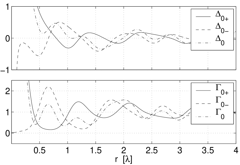
Figure 5: For $N=10$ outer atoms, the level shifts $\widetilde{\Delta}_{0\pm}$ exhibit level crossing twice on every wavelength, for $r\geq\lambda$. At the radius $r$ of a crossing, the beat frequency (90) vanishes, preventing any oscillatory population transfer between $\left|\mathcal{C}_{0}\right\rangle$ and $\left|\mathcal{C}_{z}\right\rangle$. The states $\left|\mathcal{C}_{0\pm}\right\rangle$ are defined such that, as $r\rightarrow 0$, the level shifts $\widetilde{\Delta}_{0\pm}$ tend to $\pm\infty$, respectively. — Plotted are relative quantities $\widetilde{\Delta}_{0\pm}/\Gamma$ and $\Gamma_{0\pm}/\Gamma$. For comparison, level shifts and decay rates of the state $\left|\mathcal{C}_{0}\right\rangle$ without central atom are included.

For radii greater than a certain lower bound $r_{0}$, which depends on the number $N$ of outer atoms, we see two level-crossings per unit wavelength. For $N=10$ this radius is roughly $r_{0}\sim\lambda$. At each crossing we have to reverse the assignment of square roots to eigenvalues in order to obtain smooth eigenvalues. We therefore have to redefine $\mu_{0\pm}$, and the associated eigenvectors, in order to take account of this reversal at each crossing. The final task is then to uniquely determine which of these smooth eigenvalues is to be labelled $\mu_{0+}$ and $\mu_{0-}$. A look at Fig. 5 shows that, for $r\leq 0.7\lambda$, no crossings occur, so that we can uniquely identify the eigenvalues by their behaviour in the limit $r\rightarrow 0$. In this spirit we finally define $\mu_{0\pm}$ to be that eigenvalue whose associated level shift $\widetilde{\Delta}_{0\pm}=-\Gamma\mathfrak{Re}\!~{}\mu_{0\pm}/2$ tends towards $\pm\infty$, respectively. Physically, the dipoles in the associated state $\left|\mathcal{C}_{0+}\right\rangle/\left\|\mathcal{C}_{0+}\right\|$ are aligned parallely, which in the limit $r\rightarrow 0$ produces Coulomb repulsion, and hence the positive level shift. It follows that the state $(p=0+)$ is the natural analogue of the $(p=0)$ state in configuration (b), since they both have the same behaviour at small radii. It is also expected to decay much faster than a single atom, an expectation which is indeed confirmed by the behaviour of the imaginary part $\mathfrak{Im}\!~{}\mu_{0+}=\Gamma_{0+}/\Gamma$, which tends to $\sim N+1$ as $r\rightarrow 0$. Again this follows the pattern of the $p=0$ state in configuration (b). A visual comparison between states $(p=0+)$ and $(p=0)$ is given in Fig. 5 for $N=10$ outer atoms.

On the other hand, in the state $\left|\mathcal{C}_{0-}\right\rangle/\left\|\mathcal{C}_{0-}\right\|$, the central atom is now oriented antiparallelly to the common orientation of the outer dipoles, and, in the limit $r\rightarrow 0$, is much stronger occupied than the outer atoms, as follows from eq. (80). Hence, as a consequence of Coulomb attraction between the outer atoms and the central atom, the energy is shifted towards $-\infty$, and at the same time, the system has become extremely stable against spontaneous decay: This is reflected in the fact that, as $r\rightarrow 0$, the decay rate $\Gamma_{0-}$ tends to zero as well.

As mentioned above, the states with higher quantum numbers $p=1,\ldots,N-1$ are the same as in configuration (b), and have the same eigenvalues. The two levels $p=(0\pm)$ are non-degenerate, except for accidental degeneracy, and also are non-degenerate with the $(p>0)$ levels. As a consequence, the level degeneracy is similar to case (b), and is again expressed in Table 1.

In a Gedankenexperiment we may think of switching off the coupling of the central atom to the radiation field; in this case $\mathcal{R}_{Az}=0$, hence $\widehat{\theta}=0$, and the energy eigenstates coincide with $\left|\mathcal{C}_{0}\right\rangle$ and $\left|\mathcal{C}_{z}\right\rangle$. As soon as the central atom ”feels” the radiation field, the true eigenstates are (non-unitarily) rotated away from this basis. The modulus $|\tan\widehat{\theta}|$ of the tangens of the mixing angle $\widehat{\theta}$ may be taken as a measure of the degree of correlation between the two ”unperturbed” states $\left|\mathcal{C}_{0}\right\rangle$ and $\left|\mathcal{C}_{z}\right\rangle$, or as a measure of the strength of the interaction that couples the two states. Alternatively, we could take the beat frequency $\omega_{R}$ of the oscillation between the two unperturbed states as a correlation measure:

VI.4 Quantum beats between unperturbed $p=0$ states

As follows from eqs. (80), the true eigenstates $\left|\mathcal{C}_{0\pm}\right\rangle$ are in general linear combinations of the ”unperturbed” irreducible basis vectors $\left|\mathcal{C}_{0}\right\rangle$, eq. (69), and $\left|\mathcal{C}_{z}\right\rangle$, eq. (70); as a consequence, the true eigenstates will give rise to quantum beats between $\left|\mathcal{C}_{0}\right\rangle$ and $\left|\mathcal{C}_{z}\right\rangle$. In order to determine the beat frequency we compute the amplitude for the transition $\left|\mathcal{C}_{z}\right\rangle\rightarrow\left|\mathcal{C}_{0}\right\rangle$ [both states being normalized], using eq. (18),

$$\left\langle\mathcal{C}_{0}\right|U(t,0)\left|\mathcal{C}_{z}\right\rangle=\left\langle\mathcal{C}_{0}|\mathcal{C}_{0+}\right\rangle\,e^{-\frac{i}{\hbar}\Lambda_{0+}t}\,\left\langle\mathcal{C}_{0+}^{*}|\mathcal{C}_{z}\right\rangle+\left\langle\mathcal{C}_{0}|\mathcal{C}_{0-}\right\rangle\,e^{-\frac{i}{\hbar}\Lambda_{0-}t}\,\left\langle\mathcal{C}_{0-}^{*}|\mathcal{C}_{z}\right\rangle\quad,$$ (86)

where

$$\Lambda_{0\pm}=\widetilde{E}_{i}-\frac{\hbar\Gamma}{2}\,\mu_{0\pm}\quad,$$ (87)

as follows from eqs. (39, 40). Using (80, 82) and (87) we obtain

$$P_{\left|\mathcal{C}_{z}\right\rangle\rightarrow\left|\mathcal{C}_{0}\right\rangle}(t)=\Big{|}\left\langle\mathcal{C}_{0}\right|U(t,0)\left|\mathcal{C}_{z}\right\rangle\Big{|}^{2}=\left|\sin\widehat{\theta}\cos\widehat{\theta}\right|^{2}\,\Bigg{\{}e^{-\Gamma_{0+}t}+e^{-\Gamma_{0-}t}-2\,e^{-\frac{1}{2}\left(\Gamma_{0+}+\Gamma_{0-}\right)t}\,\cos\left[\left(\widetilde{\Delta}_{0+}-\widetilde{\Delta}_{0-}\right)t\right]\Bigg{\}}\quad.$$ (88)

The last term shows that the oscillation between the two states occurs at the beat frequency

$$\omega_{R}=\left|\widetilde{\Delta}_{0+}-\widetilde{\Delta}_{0-}\right|\quad.$$ (89)

The beat frequency can be expressed in terms of the function $M$, eq. (35), as

$$\omega_{R}=\frac{\Gamma}{2}\mathfrak{Re}\!~{}\sqrt{\left[\sum_{A=2}^{N}M\left(k_{eg}R_{1A}\right)\right]^{2}+4N\,M^{2}\left(k_{eg}r\right)}\quad.$$ (90)

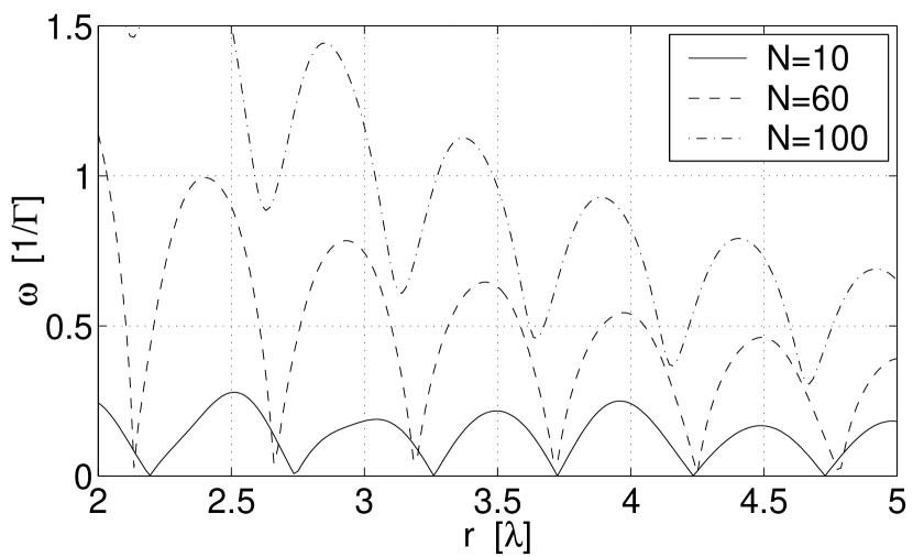
Figure 6: The beat frequency eq. (90) for three different values $N=10,60,100$ of outer atoms, for radii between $2$ and $5$ wavelengths. At the radius of a level crossing $\widetilde{\Delta}_{0+}=\widetilde{\Delta}_{0-}$, the beat frequency vanishes. It can be seen that the greater the number of outer atoms $N$, the greater becomes the radius $r_{0}$ beyond which level crossing occurs.

For a given number of outer atoms, there can exist discrete radii at which the beat frequency $\omega_{R}$ vanishes. From formula (89) we see that this is the case precisely when the two levels cross, and hence the normalized states $\left|\mathcal{C}_{0+}\right\rangle$ and $\left|\mathcal{C}_{0,-}\right\rangle$ are degenerate in energy. This is demonstrated in Figs. 5 and 6.

The beat frequency $\omega_{R}$ so computed has to be treated with a grain of salt, however. The reason is that the dynamics in the radiationless $Q$-space does not preserve probability flux, since the latter decays into the $P$-space when occupying the modes of outgoing photons. This is reflected in the presence of damped exponentials in formula (88). Depending on the number of atoms involved and the radius of the circle, this damping may be so strong, compared to the amplitude of the beat oscillations, that the dynamical behaviour effectively becomes aperiodic, i.e., exhibits no discernable oscillations. An example is given by the $N=10$ plot in Figure 7.

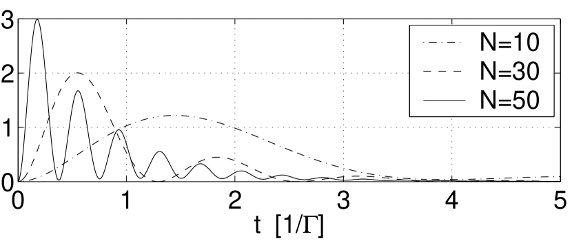
Figure 7: The probability $P(t)/|\sin\widehat{\theta}\cos\widehat{\theta}|^{2}$ for the transition $\left|\mathcal{C}_{z}\right\rangle\rightarrow\left|\mathcal{C}_{0}\right\rangle$, as given in eq. (88), for $N=10,30,50$ outer atoms. The quantum beats for $N=10$ are practically invisible, making the transfer effectively aperiodic.

VI.5 Analogy between $p=0$ states and hydrogen-like $s$ states

It is interesting to note that for the $p\neq 0$ states, the central atom is unoccupied, irrespective of the radius of the circle, or the number of atoms in the configuration. This means that the central atom takes part in the dynamics only in a $p=0$ state. This is strongly reminiscent of the behaviour of single-particle wavefunctions in a Coulomb potential, such as a spinless electron in a hydrogen atom: In this case, the electronic wavefunction vanishes at the origin of the coordinate system, i.e., at the center-of-symmetry of the potential, for all states with orbital angular momentum quantum number greater than zero. On the other hand, in the case of our planar atomic system, the circular configurations also have a center-of-symmetry, namely the center of the circle; and, as we have remarked earlier, we can interpret the single-excitation correlated states $\left|\mathcal{C}_{p}\right\rangle/\left\|\mathcal{C}_{p}\right\|$ as wavefunctions of a single quasi-particle which is distributed over the set of discrete locations $\mathbf{R}_{z},\mathbf{R}_{A}$ corresponding to the sites of the atoms. Then the amplitudes $\left\langle A,0|\mathcal{C}_{p}\right\rangle=c^{p}_{A}$ play a role analogous to a spatial wavefunction $\left\langle\mathbf{x}|\psi\right\rangle=\psi(\mathbf{x})$; and just as the hydrogen-like wavefunctions vanish at the origin for angular momentum quantum numbers $l\neq 0$ Bransden and Joachain (2003), so vanish our quasi-particle wavefunctions at the central atom for all quantum numbers other than $p=0$. In both cases, the associated wave functions are isotropic: The $s$ states transform under the identity representation ($l=0$) of $SO(3)$ in the case of hydrogen, and states $\left|\mathcal{C}_{0(\pm)}\right\rangle$ under the identity representation $(p=0)$ of $\mathbb{Z}_{N}$ in the case of our circular configurations. This means that the quantum number $p$ is analogous to the angular momentum quantum number $l$ in the central-potential problem; with hindsight, this is not surprising, since both quantum numbers $p$ and $l$ are indices which label the unitary irreducible representations of the associated symmetry groups $\mathbb{Z}_{N}$ and $SO(3)$, and in both cases a rotational symmetry is involved.

VII Exponential photon trapping in the circular configuration

In this section we are interested in the photon-trapping capability of maximally subradiant states in the circular configuration, for large numbers of atoms in the circle. To this end we choose a fixed radius, increase the number of atoms in the configuration gradually, and, for each number $N$, compute the decay rate $\Gamma_{{\text{min}}}$ of the maximally subradiant state for the given pair $(r,N)$, in configuration (b) only. We then expect a more or less monotonic decrease of $\Gamma_{\text{min}}$ as $N$ increases. But what precisely is the law governing this decrease? A numerical investigation gives the following result: In Fig. 8(a) we plot the negative logarithm $-\ln(\Gamma_{\text{min}}/\Gamma)$ of the minimal relative decay rate at the radii $r=1,1.5,2,2.5~{}\lambda$ for increasing numbers of atoms. We see that from a certain number $N=\hat{N}$ onwards, which depends on the radius, $-\ln(\Gamma_{\text{min}}/\Gamma)$ increases approximately linearly with $N$; in the figure, we have roughly $\hat{N}=14$ for $r=\lambda$, $\hat{N}=20$ for $r=1.5~{}\lambda$, $\hat{N}=26$ for $r=2~{}\lambda$, $\hat{N}=33$ for $r=2.5~{}\lambda$. We also see that the slope is a function of the radius $r$.

We note that the four curves in Fig. 8(a) imply the existence of a common critical interatomic distance: For large $N$, the next-neighbour distance $R_{nn}$ between two atoms on the perimeter of the circle is roughly equal to $2\pi r/N$; if we compute this distance for the pairs of values $(r,\hat{N})$ as found above we obtain $R_{nn}=0.45,0.47,0.48,0.48~{}\lambda$, respectively. We see that a critical distance of $R_{c}\approx 0.5~{}\lambda$ presents itself: If, for fixed radius $r$, the number of atoms in the configuration is increased, the next-neighbour distance $R_{nn}$ decreases; as soon as $R=R_{c}$ is reached, the order of magnitude by which spontaneous emission from the maximally subradiant state is suppressed becomes approximately proportional to $N$.

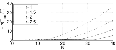
(a) Circular configuration, without central atom

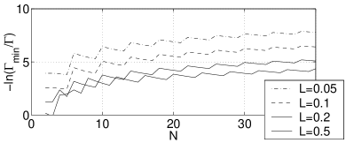
(b) Linear-chain configuration)

Figure 8: The negative logarithm of the minimal relative decay rate, being proportional to the order of magnitude of suppression of spontaneous decay, as a function of $N$, for fixed radii of the circle in Fig. 8(a), and for fixed length $L$ of the linear-chain, in Fig. 8(b). In Fig. 8(a) we see that for each radius there exists a critical number $\hat{N}$ of atoms in the configuration beyond which the order of magnitude by which spontaneous emission is suppressed is roughly proportional to $N$. In the Figure, these critical values are roughly at $\hat{N}=14,20,26,33$ atoms. Beyond these values, the next-neighbour distance, which is roughly equal to $2\pi r/N$, becomes smaller than the critical distance $\lambda/2$. – In Fig. 8(b), the same analysis is shown for four different lengths of the linear chain. A linear regime is still visible, but both the slopes of the plots, as well as the order of magnitude by which spontaneous decay is suppressed, is visibly smaller than in the circular configuration.

Based upon this reasoning we see that, for a given radius $r$, the critical number $\hat{N}$ of atoms in configuration (b) is given by $\hat{N}=\frac{4\pi r}{\lambda}$. Then, we infer from Fig. 8(a) that, approximately,

$$\Gamma_{\text{min}}\simeq\Gamma\cdot e^{-s(r)(N-\hat{N})}\quad,\quad\text{for $N>\hat{N}$}\quad,$$ (91)

where $s(r)$ determines the slopes of the curves in Fig. 8(a); this function decreases monotonically with $r$. We must have the limit $s(r)\xrightarrow{r\rightarrow\infty}0$, because for large radii all correlations between atoms must cease to exist, and hence $\Gamma_{\text{min}}\rightarrow\Gamma$ in this limit. Let $\tau\equiv 1/\Gamma$ denote the lifetime of the excited level in a single two-level atom; then formula (91) tells us that the lifetime $\tau_{\text{min}}$ of a maximally subradiant state pertaining to $\Gamma_{\text{min}}$ increases exponentially with the number of atoms,

$$\tau_{{\text{min}}}=\tau\cdot e^{s(r)(N-\hat{N})}\quad,\quad\text{for $N>\hat{N}$}\quad.$$ (92)

VIII Photon trapping in the linear chain configuration

In this last section we study a configuration of $N$ identical two-level systems which are arranged in a linear-chain configuration. As before we focus attention on simply-excited states only. This system no longer has a symmetry group, so that we have to resort to numerical methods to compute energy eigenvectors and eigenvalues. It turns out that the eigenvectors, i.e., the coefficients of the correlated states $\left|\mathcal{C}\right\rangle$ in the uncorrelated basis $\left|A,0\right\rangle$, are qualitatively very similar to those seen in Fig. 3 for the circular configurations, except for some possible modifications at the boundaries of the configuration. The energy eigenvalues exhibit a different behaviour compared to the circular system, though. The most notable difference is the occurrence of a region $d\in[0,d^{\prime}]$, $d^{\prime}<\lambda/2$, in which spontaneous decay can be strongly suppressed for the state which, for the given distance $d$, has the minimal decay rate $\Gamma_{\text{min}}$. This is shown in Fig. 9. Furthermore, in the limit $N\rightarrow\infty$, the value of $d^{\prime}$ approaches $\lambda/2$; and, as soon as $d=\lambda/2$ is approached and exceeded, the minimal decay rate exhibits a jump-like behaviour. This indicates that, even though spontaneous decay is suppressed for $d<d^{\prime}$, this suppression will become increasingly unstable, and susceptible to environmental perturbations, as soon as we approach the critical value $\lambda/2$. In the region below this critical distance, spontaneous decay may be suppressed by several orders of magnitude; for example, for the three values of $N=5,10,100$ as shown in Fig. 9, we have at the distance $d=0.25\,\lambda$ minimal decay rates of $\Gamma_{\text{min}}\sim 10^{-2},10^{-3},10^{-7}$, respectively.

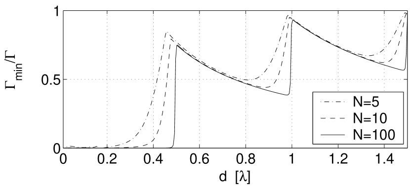
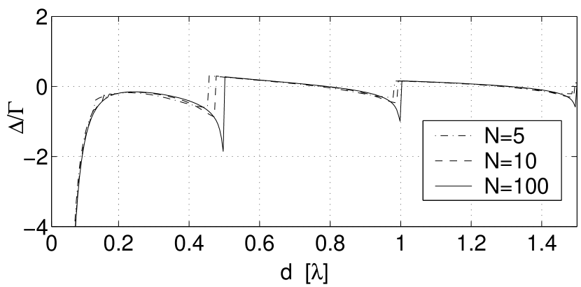
Figure 9: The minimal decay rate in the linear chain configuration c), for next-neighbour distances $d$ ranging between $0$ and $1.5\,\lambda$, and $N=5,10,100$ atoms in the chain, respectively. For $d<\lambda/2$ there is substantial suppression of spontaneous decay even for relatively small numbers $N$ of atoms.

However, the photon-trapping properties of the linear chain are not nearly as pronounced as those of the circular configurations. In Fig. 8(b) we plot the same quantities as in Fig. 8(a) but for the linear chain with a prescribed length, fixed at values of $L=0.05,0.1,0.2,0.5$ wavelengths. We see that a linear regime exists here as well, but the suppression of spontaneous decay is visibly smaller than in the circular configuration, as $-\ln(\Gamma_{\text{min}}/\Gamma)$ does not exceed a value of $10$ in the linear chain, while it reaches close to $40$ in the circle. To further exemplify this point, let us prescribe a number of, say, $N=40$ atoms, and demand a degree of suppression of spontaneous decay of, say, $-\ln\left(\Gamma_{\text{min}}/\Gamma\right)=5$. We then ask: how small must the next-neighbour distance between atoms in the circle on the one hand, and the linear-chain configuration on the other hand, be in order to achieve the prescribed suppression of radiative decay? A short computation shows that for the circle we need a next-neighbour distance $R_{nn}\simeq 2\pi r/N\sim 0.4\lambda$; while in the linear-chain configuration, $d_{nn}\simeq 0.005\lambda$ is required. In other words, it is much harder to achieve the same degree of photon trapping in the linear chain, and indeed, for the values of parameters as given above, the circular configuration performs better than the linear chain by a factor $0.4/0.005=80:1$! Thus, if our objective is photon trapping, the circular configurations definitely would be our first choice.

IX Summary

We develop the theory of simply-excited correlated states, their level shifts and decay rates, for planar configurations of identical two-level systems with parallel dipole moments, and apply the results to circular and linear configurations of atoms. For the circular systems, the atomic state space can be decomposed into carrier spaces pertaining to the various irreducible representations of the symmetry group $\mathbb{Z}_{N}$ of the system. Accordingly, the channel Hamiltonian on the radiationless subspace can be diagonalized on each carrier space separately, making an analytic computation of eigenvectors and eigenvalues feasable. Each eigenvector can be uniquely labeled by the index $p$ of this representation. For quantum numbers $p>0$ the circular configuration is insensitive to the presence or absence of a central atom, so that the wavefunction of the associated quasi-particle describing the collective excitation of the sample occupies the central atom only in a $p=0$ state. It is explained how this feature is analogous to the behaviour of hydrogen-like $s$ states in a central potential. The presence of a central atom in the circular configurations causes level splitting and -crossing of the $p=0$ state, in which case damped quantum beats between two ”extreme” $p=0$ configurations occur. For strong damping, the population transfer between the two extreme configurations is effectively aperiodic. Finally, a critical number of atoms, corresponding to a next-neighbour distance of $\lambda/2$ on the circle, exists, beyond which the lifetime of the maximally subradiant state increases exponentially with the number of atoms in the circle. The significance of this critical distance is exemplified by the jump-like behaviour of the minimal decay rate in linear-chain configurations of atoms with next-neighbour distance close to $\lambda/2$. It is demonstrated that the photon-trapping capability of the circular system is pronouncedly better than that of the linear-chain configurations.

X Appendix

Here we prove a technical result which is used in the main part of the paper:

Let $R_{1A}$ denote the distance between atoms $1$ and $A$ (i.e., outer atoms only). Let $F$ be any function of this distance, $F=F(R_{1A})$. Let $p$ be an integer. Then

$$\sum_{A=2}^{N}F(R_{1A})\,\sin\left(\frac{2\pi p}{N}(A-1)\right)=0\quad.$$ (93)

Proof:

The sum $S$ on the left-hand side of (93) can be written as

$$S=\sum_{A=2}^{N}F(R_{1,N-A+2})\,\sin\left(\frac{2\pi p}{N}(N-A+1)\right)\quad.$$ (94)

The sines are equal to

$$\sin\left(\frac{2\pi p}{N}(N-A+1)\right)=-\sin\left(\frac{2\pi p}{N}(A-1)\right)\quad,$$ (95)

while the distances satisfy the equations

$$R_{1,N-A+2}=R_{1A}\quad.$$ (96)

If this is inserted into (94) we obtain an expression which is the negative of (93), and as a consequence, $S$ must be zero. $\blacksquare$