Nonadiabatic geometric phase induced by a counterpart of the Stark shift

Abstract

We analyse the geometric phase due to the Stark shift in a system composed of a bosonic field, driven by time-dependent linear amplification, interacting dispersively with a two-level (fermionic) system. We show that a geometric phase factor in the joint state of the system, which depends on the fermionic state (resulting form the Stark shift), is introduced by the amplification process. A clear geometrical interpretation of this phenomenon is provided. We also show how to measure this effect in an interferometric experiment and to generate geometric “Schrödinger cat”-like states. Finally, considering the currently available technology, we discuss a feasible scheme to control and measure such geometric phases in the context of cavity quantum electrodynamics.

Pacs Numbers: 03.65.Vf, 42.50.Ct, 42.50.Pq

Jornal Ref. Europhys. Lett. 72, 21 (2005)

Geometric phases have been studied more widely since the seminal work of Berry Berry , in which he showed that a state, under an adiabatic and cyclic evolution, acquires a phase of geometric origin that depends on its path in the parameter space. This concept has been generalized in several ways Shapere ; Ben-Aryeh , including noncyclic noncyclic , nonadiabatic nonadiabatic , mixed state mixed and open system open evolution. More recently the interest in geometric phases has grown, owing to possible applications in quantum computation Vedral1 .

In the present paper, the geometric phase induced by a counterpart Stark shift is investigated. We consider the dispersive interaction of a two-level (fermionic) system with a quantized bosonic field driven by a time-dependent (TD) linear amplification process. A nonadiabatic geometric phase factor in the state of the system, which depends on the fermionic state, arises from the TD linear amplification. This effect is due to distinct shifts in the field frequency introduced by the different states of the two-level system (a counterpart of the Stark shift) and it can be measured by an interferometric experiment. We can interpret the origin of this phenomenon as a consequence of the different projective maps associated with the dynamics of the two fermionic states. Although, in general, the calculation of geometric phases in the nonadiabatic case is not an easy task, the TD invariants technique of Lewis and Riesenfeld Lewis provides an easy and direct way to obtain such phases Salomon ; Mostafazadeh .

We also propose a scheme, employing cavity quantum electrodynamics (QED) and considering currently available technology Haroche1 ; Haroche2 ; Walther , by which such phases can be generated, manipulated, and tested. Recent advances in this context have led to striking experiments that afforded fundamental tests of quantum theory Haroche1 ; Haroche2 ; Haroche3 ; Walther , as well as motivating several theoretical proposals. Carollo et al. Carollo1 proposed an experiment to measure the adiabatic geometric phase induced by the vacuum state Carollo2 when a two-level atom interacts resonantly with two quantized modes in a cavity. In Ref. Serra1 the authors show, in a Jaynes-Cummings-like model, how to simulate anyonic behavior and how to transmute the statistics of the atom-field system via the adiabatic geometric phase.

Assuming that the transition frequency of the two-level system $\omega_{0}$ is detuned enough from the bosonic field frequency $\nu$ Scully , the effective Hamiltonian for the dispersive interaction between the two-level system and the field mode under TD linear amplification process, is given by ($\hbar=1$)

$$\widehat{H}\left(t\right) =\nu\widehat{a}^{\dagger}\widehat{a}+\frac{\omega_{0}}{2}\widehat{\sigma}_{z}+\chi\widehat{a}^{\dagger}\widehat{a}\widehat{\sigma}_{z}+\chi\widehat{\sigma}_{ee}$$

$$+f(t)\widehat{a}^{\dagger}+f^{\ast}(t)\widehat{a}\text{,}$$ (1)

where $\chi$ is the effective dispersive coupling constant Scully ; Haroche2 , $\widehat{\sigma}_{z}=\left|e\right\rangle\left\langle e\right|-\left|g\right\rangle\left\langle g\right|$ is the usual Pauli pseudo-spin operator, $\widehat{\sigma}_{ee}=\left|e\right\rangle\left\langle e\right|$ ($\left|e\right\rangle$ and $\left|g\right\rangle$ are the excited and ground states of the two-level system, respectively), $\widehat{a}^{\dagger}$ ($\widehat{a}$) is the creation (annihilation) field operator and $f(t)$ is the TD complex amplitude of the linear amplification.

The state vector of the Schrödinger equation associated with Hamiltonian (1) can be written as Celso

$$\left|\Psi(t)\right\rangle=e^{i\omega_{0}t/2}\left|g\right\rangle\left|\Phi_{g}(t)\right\rangle+e^{-i\left(\omega_{0}/2+\chi\right)t}\left|e\right\rangle\left|\Phi_{e}(t)\right\rangle,$$ (2)

with $|\Phi_{\ell}\left(t\right)\rangle=\widehat{1}_{a}\otimes\left\langle\ell\right.|\Psi\left(t\right)\rangle$ ($\ell=e,g$), $\widehat{1}_{a}$ being the unitary operator of field mode $a$ represented in a convenient basis. Using the orthogonality of the fermionic states in $|\Psi\left(t\right)\rangle$ we obtain the uncoupled TD Schrödinger equations for the bosonic field states:

$$i\frac{\partial}{\partial t}\left|\Phi_{\ell}(t)\right\rangle=\widehat{\mathrm{H}}_{\ell}(t)\left|\Phi_{\ell}(t)\right\rangle,$$ (3)

where

$$\widehat{\mathrm{H}}_{\ell}(t)=\varpi_{\ell}\widehat{a}^{\dagger}\widehat{a}+f(t)\widehat{a}^{\dagger}+f^{\ast}(t)\widehat{a},$$ (4)

with $\varpi_{e}=\nu+\chi,$ and $\varpi_{g}=\nu-\chi$. Now, the problem has been reduced to that of a harmonic oscillator under linear amplification, whose frequency $\nu$ is shifted by $\chi$ ($-\chi$) when interacting with the state $\left|e\right\rangle$ ($\left|g\right\rangle$) Celso .

We will employ the TD invariants technique to solve exactly Hamiltonian (4) and obtain the geometric phase associated with the states $\left|e\right\rangle$ and $\left|g\right\rangle$. From the well-known theorem of Lewis and Riesenfeld (LR) Lewis it follows that the general solution of the TD Schrödinger equation (3), given by $\left|\Phi_{\ell}(t)\right\rangle=\sum_{m}c_{\ell,m}\exp\left[i\phi_{\ell,m}(t)\right]\left|m,t\right\rangle_{\ell},$ comprehends a superposition of the eigenstates $\left|m,t\right\rangle_{\ell}$ of the Hermitian invariant $I_{\ell}(t)$ ($dI_{\ell}(t)/dt\equiv\partial I_{\ell}(t)/\partial t+i\left[\widehat{\mathrm{H}}_{\ell}(t),I_{\ell}(t)\right]=0$) multiplied by the TD phase factor $\phi_{\ell,m}(t)=\phi_{\ell,m}^{D}(t)+\phi_{\ell,m}^{G}(t)$; one of those components is dynamic:

$$\phi_{\ell,m}^{D}(t)=-\int_{0}^{t}dt^{\prime}\;_{\ell}\left\langle m,t^{\prime}\right|\widehat{\mathrm{H}}_{\ell}(t^{\prime})\left|m,t^{\prime}\right\rangle_{\ell},$$ (5)

and the other is geometric Salomon ; Mostafazadeh :

$$\phi_{\ell,m}^{G}(t)=i\int_{0}^{t}dt^{\prime}\;_{\ell}\left\langle m,t^{\prime}\right|\frac{\partial}{\partial t^{\prime}}\left|m,t^{\prime}\right\rangle_{\ell}.$$ (6)

The geometric phase in this formulation arises from a holonomy over the parameter space associated with the invariant $I_{\ell}(t)$ Salomon ; Mostafazadeh . By this method, it is possible to compute the geometric phase in a general scenario, including adiabatic and nonadiabatic evolutions of pure states.

The invariant $I_{\ell}(t)$ associated with Hamiltonian (4) is given by Puri

$$I_{\ell}(t)=\widehat{a}^{\dagger}\widehat{a}-\alpha_{\ell}(t)\widehat{a}^{\dagger}-\alpha_{\ell}^{\ast}(t)\widehat{a}+\beta_{\ell}(t),$$ (7)

and the invariant $\mathcal{I}(t)$ related to the total Hamiltonian (1) is $\mathcal{I}(t)={\displaystyle\sum\limits_{\ell=g,e}}I_{\ell}(t)\left|\ell\right\rangle\left\langle\ell\right|,$ where the coefficients $\alpha_{\ell}(t)$ and $\beta_{\ell}(t)$ satisfy the coupled equations

$$\overset{.}{\alpha_{\ell}}(t) =-i\varpi_{\ell}\alpha_{\ell}(t)-if(t),$$ (8a)

$$\overset{.}{\beta_{\ell}}(t) =i\alpha_{\ell}(t)f^{\ast}(t)-i\alpha_{\ell}^{\ast}(t)f(t).$$ (8b)

The eigenstates of the invariant $I_{\ell}(t)$ are the displaced number states $\left|m,t\right\rangle_{\ell}=\widehat{D}\left[\alpha_{\ell}(t)\right]\left|m\right\rangle$ where $\widehat{D}\left[\alpha_{\ell}(t)\right]=\exp\left[\alpha_{\ell}(t)\widehat{a}^{\dagger}-\alpha_{\ell}^{\ast}(t)\widehat{a}\right]$ and $\alpha_{\ell}(t)$ is the TD complex amplitude

$$\alpha_{\ell}(t)=\alpha_{\ell}(0)e^{-i\varpi_{\ell}t}-ie^{-i\varpi_{\ell}t}\int_{0}^{t}e^{i\varpi_{\ell}t^{\prime}}f(t^{\prime})dt^{\prime}.$$ (9)

Let us suppose that the fermionic particle is prepared initially in the superposition state $c_{g}\left|g\right\rangle+c_{e}\left|e\right\rangle$ while the field is in the vacuum state $\alpha_{\ell}(0)=0$. For our purpose we adjust the temporal dependence of the linear amplification to resonance with the field mode, such that $f(t)=\kappa e^{-i\nu t}$. In order to clarify the contributions of the geometric and the dynamic phases we write the vector state of the system

$$\left|\Psi(t)\right\rangle =e^{i\phi^{D}(t)}\left(C_{g}(t)e^{i\phi_{g}^{G}(t)}\left|\alpha_{g}(t)\right\rangle\left|g\right\rangle\right.$$

$$\left.+C_{e}(t)e^{i\phi_{e}^{G}(t)}\left|\alpha_{e}(t)\right\rangle\left|e\right\rangle\right),$$ (10)

where $C_{g}(t)=c_{g}\operatorname*{e}\nolimits^{i\omega_{0}t/2}$, $C_{e}(t)=c_{e}\operatorname*{e}\nolimits^{-i\left(\omega_{0}/2+\chi\right)t}$, and the amplitudes of the coherent states $\alpha_{\ell}(t)$ are given by

$$\alpha_{\left(\genfrac{}{}{0.0pt}{}{g}{e}\right)}(t)=\pm\frac{\kappa}{\chi}e^{-i\nu t}(1-e^{\pm i\chi t}).$$ (11)

The geometric phases associated with the ground and excited states are note1

$$\phi_{\binom{g}{e}}^{G}(t)=\left(2\nu\mp\chi\right)\left(\frac{\kappa}{\chi}\right)^{2}\left[t-\frac{\sin(\chi t)}{\chi}\right],$$ (12)

while the factorized dynamic phase turns out to be

$$\phi^{D}(t) =\phi_{g}^{D}(t)=\phi_{e}^{D}(t)$$

$$=-2\nu\left(\frac{\kappa}{\chi}\right)^{2}\left[t-\frac{\sin(\chi t)}{\chi}\right].$$ (13)

We note that, for the choice of the parameters considered above, the dynamic phase remains factorized during the whole time evolution of the system, as shown in Eq. (10), when the field mode is initially in the vacuum state $\alpha_{\ell}(0)=0$; otherwise $\phi_{g}^{D}(t)\neq\phi_{e}^{D}(t)$. On the other hand, the geometric phase depends on the fermionic state, i.e., on the shift of the field frequency introduced by the fermionic particle.

Unlike the states of an isolated two-level system which can simply be described on Bloch’s sphere, in the present context a representation of the geometrical phase associated with the evolution of the entangled state (10) is supplied by getting rid of the fermionic degree of freedom and making use of the quantum phase space associated with the field mode. From this perspective, the dependence of the geometrical phase (12) upon the state of the two-level system can be visualized in the projective map $\Gamma_{\ell}$ of the Hilbert space $\mathcal{H}_{\ell}$ into the projective space $\mathcal{P}_{\ell}$ [$\Gamma_{\ell}:\mathcal{H}_{\ell}\longrightarrow\mathcal{P}_{\ell}$ ($\ell=e,g$)].  In fact, the Hamiltonian (4) is different for each fermionic subspace, although the parameter space is the same.

In Fig. 1 we present the typical spiraling path followed by the coherent states $\left|\alpha_{\ell}(t)\right\rangle$, associated with the fermionic levels $e$ and $g$, during a half cycle ($\chi t\in[0,\pi]$) in the phase space $\operatorname{Re}\left\{\left(\chi/\kappa\right)e^{i\upsilon t}\alpha_{\ell}(t)\right\}\times\operatorname{Im}\left\{\left(\chi/\kappa\right)e^{i\upsilon t}\alpha_{\ell}(t)\right\}$. In this figure, we can see that the trajectory of state $\left|\alpha_{e}(t)\right\rangle$ performs an extra half loop in the phase space compared to state $\left|\alpha_{g}(t)\right\rangle$, during a half cycle. This occurs due to the different signals in Eq. (11) which arise in the distinct frequency shifts of the effective Hamiltonian (4). Summarizing, since the fermionic states introduce distinct shifts in the bosonic field, the paths in the phase space associated to the respective fermionic subspaces differ by one loop around the origin during one cycle.

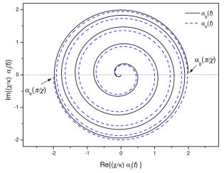
Figure 1: Typical path followed by the amplitudes $\alpha_{g}(t)$ and $\alpha_{e}(t)$ of the coherent states in the phase space for $\chi t\in\left[0,\pi\right]$.

Let us consider the projective space associated with the instantaneous eigenstates $\left|m,t\right\rangle_{\ell}$ of the invariant $I_{\ell}(t)$. From the coupled equations (8a) and (8b) we can see that the quantity $\beta_{\ell}(t)-\left|\alpha_{\ell}(t)\right|^{2}$ (apart from a constant which can be considered null without loss of generality) is conserved. Due to this conservation law we can represent the state $\left|\alpha_{\ell}(t)\right\rangle$ in a surface of a hyperboloid (i.e. the Poincaré hyperboloid Ben-Aryeh ). In Fig. 2 we show the trajectories of the state $\left|\alpha_{\ell}(t)\right\rangle$ associated with each fermionic level $\ell$ in the Poincaré hyperboloid. In this figure we can clearly see that there are two different projective maps $\Gamma_{\ell}$ associated with each ferminonic state $\left|\ell\right\rangle$, introducing the effect shown in Eq. (12).

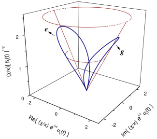
Figure 2: The path followed by the field states $\left|\alpha_{\ell}(t)\right\rangle$ associated with each fermionic level ($g$ and $e$) in the Poincaré hyperboloid during a complete cycle (considering a rotating frame with frequency $\nu$).

Now, we will discuss how to implement, in a physical context, the effect discussed above. To this end we consider the cavity QED domain. The experimental setup proposed consists in a two-level Rydberg atom which crosses a Ramsey-type arrangement (i.e., a high-Q microwave cavity $C$ placed between two Ramsey Zones $R_{1}$ and $R_{2}$) Haroche2 and is detected in the excited state ($\left|e\right\rangle$) or in the ground state ($\left|g\right\rangle$) by two ionization chambers $D_{e}$ or $D_{g}$. The linear amplification in this context is achieved by the coupling of a microwave generator to the cavity through a wave guide Haroche2 .

The geometric phase induced by a counterpart Stark shift can be verified in a typical Ramsey-type interferometric experiment Haroche2 . Let us consider the following scenario: first, the atom is prepared by a Ramsey zone $R_{1}$ in a superposition state such that $c_{g}=c_{e}=1/\sqrt{2}$. Subsequently, we assume that the microwave generator is turned on (off) suddenly at the instant the atom enters (leaves) the cavity region, so that $f(t)=0$ when the atom is outside the cavity. If the atom-field interaction time is adjusted such that $\chi t=2\pi$, the evolved state vector in the interaction picture assumes, apart from a global phase, the form $\left|\Psi_{I}(t)\right\rangle=\left(\left|g\right\rangle+\operatorname*{e}\nolimits^{i\left[\phi_{e}^{G}(t)-\phi_{g}^{G}(t)\right]}\left|e\right\rangle\right)\left|0\right\rangle/\sqrt{2}$. In the Ramsey zone $R_{2}$ a $\pi/2$ pulse [i.e. $\left|g\right\rangle\longrightarrow\left(\left|g\right\rangle+\left|e\right\rangle\right)/\sqrt{2}$ and $\left|e\right\rangle\longrightarrow\left(\left|e\right\rangle-\left|g\right\rangle\right)/\sqrt{2}$], is performed in the atomic states. Finally the experiment is repeated for different values of $\kappa$ to obtain the Ramsey fringes. In this way we can measure the atomic state in the ionization chambers $D_{e}$ and $D_{g}$, so that the atomic inversion (i.e. the difference between the detection probability of the states $\left|e\right\rangle$ and $\left|g\right\rangle$) becomes

$$W_{eg}\left(\kappa\right)=\cos\left(4\pi\frac{\kappa^{2}}{\chi^{2}}\right).$$ (14)

We note that in the present proposal the pattern of the Ramsey fringes depends on the intensity $\kappa$ of the linear amplification field (for a fixed coupling $\chi$) and not on the atom-field interaction time as usual Haroche2 . The phase factor measured here is only of geometric nature.

In cavity QED experiments we have typically $\chi\sim 10^{4}s^{-1}$ and $\nu\sim 10^{10}s^{-1}$ Haroche2 . Hence, it is possible to perform the entire cycle in Fig. 2 assuming the interaction time $t\sim 10^{-4}s$, which is much shorter than the photon decay time — of the order of $10^{-3}s$ Haroche1 ; Haroche2 for open and $10^{-1}s$ Walther for closed cavities — making the dissipative and decoherence mechanisms practically negligible. Therefore, our scheme provides a fast generation of geometric phases, in contrast with the adiabatic proposals. We observe that to obtain an argument of $2\pi$ in the cosine in Eq. (14), we need $\kappa=\chi/\sqrt{2}$ so that $\kappa\sim 10^{4}s^{-1}$ for the above parameters. In this situation the maximum amplitude of the coherent state generated in the cavity mode, occurring in the half cycle, is $\left|\alpha_{e}(t)\right|_{\max}=\left|\alpha_{g}(t)\right|_{\max}=\left|2\kappa/\chi\right|=\sqrt{2}$, so that the cavity mode has less than two photons during the whole atom-field interaction. Another error source is the imperfect synchronization between the switch on (off) of the driving field and the instant when the atom enters (leaves) the cavity, due to the spreading in the velocity of the atomic beam, which is typically (in cavity QED experiments) about $2\%$ Haroche2 . Such spreading induces a fluctuation in the time that the atom enters (leaves) the cavity about $\delta t\sim 10^{-6}s$, which leads to a small correction to the Eq. (14). When the atom enters the cavity early we have

$$W_{eg}^{early}\left(\kappa\right)\approx\cos\left[4\pi\frac{\kappa^{2}}{\chi^{2}}-2\kappa^{2}\left(\delta t\right)^{2}\right],$$ (15)

and when the atom enters the cavity late the Eq. (14) turns out to be

$$W_{eg}^{late}\left(\kappa\right)\approx\cos\left[4\pi\frac{\kappa^{2}}{\chi^{2}}-\kappa^{2}\chi\left(\delta t\right)^{3}\right].$$ (16)

From the experimental parameters above, follows that the corrections in Eqs. (15) and (16), due the imperfect synchronization, are negligible $2\kappa^{2}\left(\delta t\right)^{2}\sim 10^{-4}$ and $\kappa^{2}\chi\left(\delta t\right)^{3}\sim 10^{-6}$, respectively.

We stress that, the dispersive approximation, in the Hamiltonian (1), can safely be assumed without significant corrections to the computed geometric phase when considering the regime $\chi\geq\kappa\$and $\left(\frac{g}{\Delta}\right)^{2}\ll 1$ (where $\Delta=\nu-\omega_{0}$ is the atom-field detuning and $g$ is the dipole Rabi coupling between the levels $\left|e\right\rangle$ and $\left|g\right\rangle$). Such conclusion follows from the analysis of the motion equations for the transition operators $\left|e\right\rangle\left\langle g\right|$ and $\left|g\right\rangle\left\langle e\right|$ obtained without the dispersive approximation. Typically, in the cavity QED experiments Haroche2 ; Haroche3 , $\left(\frac{g}{\Delta}\right)^{2}\sim 10^{-3}$ and we have considered the parameter $\kappa$ satisfying the required regime.

The present interferometric device can also be employed to engineer a “Schrödinger cat”-like state whose parity depends on a geometric phase factor. If we adjust the interaction time such that $\chi t=\pi$, the evolved state vector (after the atom has crossed the Ramsey-type arrangement) turns out to be, apart from an irrelevant global phase,

$$\left|\Psi_{I}(t)\right\rangle =\frac{1}{2}\left[\left(\left|2\kappa/\chi\right\rangle+\operatorname*{e}\nolimits^{2\pi i\left(\kappa/\chi\right)^{2}}\left|-2\kappa/\chi\right\rangle\right)\left|g\right\rangle\right.$$

$$\left.+\left(\left|2\kappa/\chi\right\rangle-\operatorname*{e}\nolimits^{2\pi i\left(\kappa/\chi\right)^{2}}\left|-2\kappa/\chi\right\rangle\right)\left|e\right\rangle\right],$$ (17)

Therefore, the measurement of the atomic state projects the cavity mode into a “Schrödinger-cat”-like state with a relative phase of geometric nature.

It is worth mentioning, that the scheme presented here can be employed in other experimental contexts.

In summary, we have shown that there is a geometric phase induced by the a counterpart Stark shift and we have presented a scheme to control and measure nonadiabatic geometric phases in cavity QED which can be carried out with present-day technology. The dynamic phase in our scheme remains factorized during the whole evolution of the joint system state and, on the other hand, the geometric phases depend on the electronic states of the two-level atom. This phenomenon arises from the Stark shift induced in the field mode by a dispersive atom-field interaction. Finally, we note that this effect has a potential application in geometric quantum computation Vedral1 , an interesting topic for further investigation being the system composed by two non-resonant atoms interacting dispersively with the cavity field under linear amplification. In this case the shift in the field frequency will depend on the joint state of the atoms and, in principle, by a suitable adjustment of the parameters, a conditional operation could be obtained.

R. M. Serra acknowledge A. Carollo, D. K. L. Oi, F. L. Semião and V. Vedral for enlightening discussions. This research was supported by FAPESP, CNPq, and CAPES (Brazilian agencies).

References

- (1) M. V. Berry, Proc. Roy. Soc. London A 392, 45 (1984).
- (2) A. Shapere and F. Wilczek, Geometric phases in physics, World Scientific (Singapore, 1989).
- (3) Y. Ben-Aryeh, J. Opt. B: Quantum Semiclass. Opt. 6, R1 (2004).
- (4) J. Samuel and R. Bhandari, Phys. Rev. Lett. 60, 2339 (1988).
- (5) Y. Aharonov and J. Anandan, Phys. Rev. Lett. 58, 1593 (1987).
- (6) E. Sjöqvist, et al. Phys. Rev. Lett. 85, 2845 (2000); R. Bhandari, Phys. Rev. Lett. 89, 268901 (2002); J. Anandan, et al., Phys. Rev. Lett. 89, 268902 (2002).
- (7) A. Carollo, et al., Phys. Rev. Lett. 90, 160402 (2003); R. S. Whitney and Y. Gefen, Phys. Rev. Lett. 90, 190402 (2003); J. G. Peixoto de Faria, A. F. R. de Toledo Piza, and M. C. Nemes, Europhysics Letters 62, 782 (2003).
- (8) G. Falci, et al. Nature (London) 407, 355 (2000); A. Ekert, et al. J. Mod. Opt. 47, 2501 (2000); J. Pachos, P. Zanardi, and M. Rasetti, Phys. Rev. A 61, 010305 (2000).
- (9) H. R. Lewis Jr. and W. B. Riesenfeld, J. Math. Phys. 10, 1458 (1969).
- (10) S. S. Mizrahi, Phys. Lett. A 138, 465 (1989); X-C. Gao, J-B. Xu, and T-Z. Qian, Phys. Rev. A 44, 7016 (1991); O. Kwon, C. Ahn, and Y. Kim, Phys. Rev. A 46, 5354 (1992); D. B. Monteoliva, H. J. Korsch, and J. A. Nunez, J. Phys. A: Math. Gen. 27, 6897 (1994).
- (11) A. Mostafazadeh, J. Phys. A: Math. Gen. 32, 8157 (1999).
- (12) M. Brune, et al. Phys. Rev. Lett. 77, 4887 (1996); G. Nogues, et al. Nature (London) 400, 239 (1999); A. Rauschenbeutel, et al. Science 288, 2024 (2000).
- (13) J. M. Raimond, M. Brune, and S. Haroche, Rev. Mod. Phys. 73, 565 (2001).
- (14) M. Brune, J. M. Raimond, and S. Haroche, Phys. Rev. A 35, 154 (1987).
- (15) B. T. H. Varcoe, et al. Nature (London) 403, 743 (2000); S. Brattke, B. T. H. Varcoe, and H. Walther, Phys. Rev. Lett. 86, 3534 (2001).
- (16) A. Carollo, M. França Santos, and V. Vedral, Phys. Rev. A 67, 063804 (2003).
- (17) I. Fuentes-Guridi, et al. Phys. Rev. Lett. 89, 220404 (2002).
- (18) R. M. Serra, et al. Phys. Rev. A 70, 044102 (2004).
- (19) M. O. Scully and M. S. Zubairy, Quantum Optics, Cambridge University Press (Cambridge, UK, 1997).
- (20) C. J. Villas-Bôas, et al. Phys. Rev. A 68, 053808 (2003).
- (21) R. R. Puri and S. V. Lawande, Phys. Lett. A 70, 69 (1979).
- (22) It is important to note that, the expression (13) agree with the usual definition of the geometric phase for a noncyclic evolution, i.e. Ben-Aryeh ; Mostafazadeh , since the first term is null due to our choice of initial state (the vacuum state).