Highly Nonclassical Quantum States and Environment Induced Decoherence

Highly Nonclassical Quantum States
and Environment Induced Decoherence

Introduction

The discovery of the quantized nature of the electromagnetic radiation and atomic energies followed by the foundation of Quantum Mechanics is one of the greatest achievements in physics. Quantum theory is found to provide excellent description of fields and elementary particles as well, and it became a standard tool for investigating “microscopic” physical objects.

Dirac postulated the superposition principle to be a fundamental concept even before the canonical Hilbert-space formulation of the theory has been established. Although the predictive power of quantum mechanics is based on this principle, it is counter-intuitive for a human mind that experiences a world of classical mechanics since the beginning of consciousness. The most famous example showing the incompatibility of the superposition principle with the usual way of thinking was given by Schrödinger [1, 2], where the fate of a cat in a box is triggered by the decay of a radioactive atom. If the duration of this gedanken experiment equals to the half-life of the atom, it is obvious that the survival probability of the cat is $\frac{1}{2}$. More surprisingly, the result will be an entangled state, the superposition of a dead cat with a decayed atom and a cat alive with an undecayed atom. The two states that form the superposition – as a matter of life and death – are clearly distinct. Such a superposition of two classically distinguishable states, which is usually called a Schrödinger-cat state, is allowed in quantum systems, but never observed in everyday life. In fact, the term “classically distinguishable states” means states that can be interpreted in a classical world, where, due to the lack of the superposition principle, their superposition is not present. (Note that here and throughout this thesis the attribute “classical” stands for the opposite of “quantum”.)

In fact, most of the quantum mechanical states have properties that are unusual from the classical point of view, and therefore, in some sense, they are nonclassical. On the other hand, Schrödinger-cat states are in such a strong contradiction with the classical description of a physical system, that they can be called highly nonclassical quantum states without exaggeration. The Wigner function of these states is negative over some regions of its domain, which is the signature of (high) nonclassicality from our point of view.

An apparent implication of the quantum effects that are paradoxical from the classical point of view is that there exists a classical and a quantum realm in nature, with their respective laws. The quantum realm is usually identified with microscopic particles, but sometimes it is difficult to draw a non-flexible quantum-classical border. E.g., considering a fullerene $(\mathrm{C}_{\mathrm{60}})$ molecule, there are experimental situations, such as the scattering of highly charged ions on $\mathrm{C}_{\mathrm{60}}$, when a fully classical model provides agreement with the measured results [3]. On the other hand, this cage of $60$ carbon atoms surrounded by $360$ electrons produces interference fringes on a screen placed behind a grating [4], that is, the molecule as a whole exhibits genuinely quantum behavior.

Alternatively, we can assume that quantum mechanics is universal, and so is the superposition principle. In this case, however, the emergence of classical properties has to be explained in the framework of quantum theory. There is a name for this fundamental problem: decoherence. In other words, decoherence is the disappearance of the quantum superpositions that distinguishes a Schrödinger-cat state from the corresponding classical mixture describing a system that is either in one of the classical states or in the other. Models for decoherence usually describe it dynamically, that is, decoherence is considered as a process that is extremely fast on everyday timescales.

Besides its fundamental importance, exploring the mechanisms of decoherence can have practical applications as well. The recently born and rapidly developing field of quantum information technology relies on the quantum nature of the physical objects that store, carry and process information. This is the very origin of the classically unreachable computational power of quantum algorithms. From this point of view, decoherence is the most serious obstacle still hindering the practical use of quantum computation (QC) [5]. Knowing the way in which decoherence destroys quantum superpositions renders it possible to find promising decoherence-free states. These states are exceptionally robust, they keep their quantum properties for a time hopefully long enough for implementing quantum algorithms.

In this work we consider the decoherence model that is based on the interaction of the investigated quantum system with its unavoidably present (quantum) environment. In Chap. 1 we summarize the basic concepts of this model, which is called environment induced decoherence. Chap. 2 is devoted to the description of the methods that are useful in setting up and solving the relevant dynamical equations, which, besides realizing the conceptually important link between quantum and classical mechanics, provide a realistic description of open quantum systems.

In the second part of the thesis we use these methods in order to analyze nonclassicality and investigate the effects of decoherence in concrete quantum systems. The presented results are based on the publications [6, 7, 8, 9, 10, 11, 12, 13].

In Chap. 3 we investigate the time evolution of wave packets in the anharmonic Morse potential, which can provide a realistic model for a vibrating diatomic molecule. This chapter deals with the situation when no environmental effects are present. Using the Wigner function of the system, we show that for vibrations with amplitudes exceeding the limits of the harmonic approximation, spontaneous formation of Schrödinger-cat states occur. These highly nonclassical states are superpositions of two distinct states that are localized both in position and momentum.

As a result of the environmental influence, the Schrödinger-cat states are expected to disappear rapidly, and it is known that when the potential is is approximated by a harmonic one, the result of the decoherence will be the mixture of the constituent localized states. Our analysis in Chap. 4 shows that this is not the case for the Morse oscillator. We introduce a master equation for a general anharmonic system in interaction with a thermal bath of harmonic oscillators. Using this equation we find that decoherence drives the system into a density operator that can be interpreted as the mixture of localized states equally distributed along the phase space orbit of the corresponding classical particle. That is, the information related to the position along this orbit (“phase information”) is completely lost. On the contrary, after the process of decoherence, the energy distribution of the system is still quite sharp, in fact the expectation value of the Hamiltonian is very close to its initial value. Because of the separation of the time scales of decoherence and dissipation, these processes can be clearly distinguished. We define the characteristic time of the decoherence as the time instant when the transition between the decoherence dominated and dissipation dominated time evolution takes place.

In Chap. 5 the same definition is proven to be valid for a system of two-level atoms interacting with the free radiational field. This model offers the possibility of investigating the approach to the macroscopic limit by increasing the number of atoms. We found that the larger is this number, the more naturally ans sharply the time evolution splits into two regimes. In this physical system the atomic coherent states [14] can be given a clear classical interpretation, they correspond to certain directions of the Bloch vector [15]. Therefore superpositions of different atomic coherent states are rightly called atomic Schrödinger-cat states. We show by analytical short time calculations that the coherent constituents of these highly nonclassical states are robust against the effects of decoherence. Consequently, the decoherence of the atomic Schrödinger-cat states is expected to lead to the classical mixture of the constituent atomic coherent states. We obtain that this conjecture is true, unless decoherence is exceptionally slow. In Chap. 5 we give a scheme of decoherence that remains valid also for the so-called symmetric Schrödinger-cat states, which exhibit exceptionally slow decoherence.

The basic object which is manipulated in QC algorithms is a qubit, which is an abstract two-level quantum system. A system of two-level atoms can provide a physical realization of a sequence of qubits. The usefulness of this realization depends on the extent to which the difficulties related to the decoherence can be eliminated. In this context the the possible preparation of decoherence-free states is important, this issue is discussed in Chap. 6. We consider the atoms to be in a cavity, and propose a method that can prepare decoherence-free states. Besides the free time evolution in the cavity, our scheme requires the possibility of changing the state of one of the atoms on demand. The analysis of these requirement shows that our scheme can be implemented with present day cavity QED setups.

Chapter 1 Environment induced decoherence

The apparent lack of a superposition of macroscopically distinct quantum states (Schrödin-ger cats) has been an interesting and vivid problem since Schrödinger’s famous papers [1, 2]. A successful approach, initiated by Zeh [16] and developed by Zurek [17], obtains the loss of quantum coherence as the consequence of the inevitable interaction with the environment. Theoretical studies in this framework have investigated a variety of model systems usually coupled to a collection of harmonic oscillators as an environment. Fundamental work has been done on this subject in Refs. [18, 19, 20, 21, 22, 23, 24, 25], for reviews see [26, 27]. Important experiments have also been carried out during the last years [28, 29, 30].

We note that whatever successful is the approach of the environment induced decoherence, it is not the only possible mechanism that can explain the phenomenon of decoherence. Spontaneous collapse models are conceptually different, they are based on an appropriately modified Schrödinger equation, which automatically leads to classical behavior for large systems. We shall not consider these models here, a review can be found in Chap. 8 of Ref. [27]. The role of gravity is also often discussed in both of the two main approaches, see [31, 32, 24, 33].

1.1 Formation of system-environment entanglement

Apart from cosmology, we usually focus our interest on a specific part of the universe. This distinguished subsystem (our “system”, $S$) is, however, unavoidably coupled to the “rest of the world”, called environment ($E$) in this context. Although the way in which we single out our system can appear accidental or even artificial, it is clearly necessary to obtain a useful, solvable model. Additionally, measurements performed on $S$ are in most of the cases “local”, i.e., concern the degrees of freedom of the system only. (In fact, the definition of the “system” in a theoretical model is closely related to the possible measurements the outcomes of which are to be predicted.) Neglecting the $S$-$E$ interaction leads to results that are good approximations only for very well isolated systems and for short times. For a more realistic description of the necessarily open quantum system $S$, the effects of the environment have to be taken into account. The system-environment interaction builds up entanglement (Verschränkung) between the the two quantum systems $S$ and $E$. In order to obtain results for the system only, we have to average over the unobservable environmental degrees of freedom. This process of “tracing out the environment” (see the next chapter) provides a density operator of $S$ that usually describes a mixed state and contains all the information that can be extracted by local measurements.

In order to illustrate this concept, we consider a simple but expressive example [27, pp. 41-42] with the interaction term

$$V_{int}=\sum_{n}|n\rangle_{S}{}_{S}\langle n|\otimes B_{E}(n)=\sum_{n}|n\rangle_{S}{}_{S}\langle n|B_{E}(n)$$ (1.1)

connecting $S$ and $E$. The states $\{|n\rangle_{S}\}$ are assumed to form an orthogonal basis in the Hilbert space of the system, while $B_{E}(n)$ denote (Hermitian) environmental operators. The operators $|n\rangle_{S}{}_{S}\langle n|$ act in the Hilbert space of the system, and similarly $B_{E}(n)$ stands for the tensorial product of the identity $\mathrm{id}_{S}$ with the environmental operator $B_{E}(n)$. In what follows, when it is not necessary, the tensorial product sign will be omitted in the notation.

Note that $V_{int}$ is special in the sense that it does not contain cross terms like $|n\rangle_{S}{}_{S}\langle m|$, $n\neq m$, but it demonstrates the main effects well. Later on we shall consider more general interactions as well. As a further approximation, we neglect the self-Hamiltonians of $S$ and $E$ for the moment. Assuming an initially uncorrelated state

$$|\Psi(t=0)\rangle_{SE}=|\phi(0)\rangle_{S}|\Phi(0)\rangle_{E}=\sum_{n}c_{n}|n\rangle_{S}\ |\Phi(0)\rangle_{E},$$ (1.2)

the time evolution builds up $S$-$E$ correlations and leads to an entangled state:

$$|\Psi(t)\rangle_{SE}=\sum_{n}c_{n}|n\rangle_{S}\ e^{\frac{-iB_{E}(n)t}{\hbar}}|\Phi(0)\rangle_{E}=\sum_{n}c_{n}|n\rangle_{S}\ |\Phi\rangle_{E}^{n},$$ (1.3)

where $|\Phi\rangle_{E}^{n}=\exp(-iB_{E}(n)t/\hbar)|\Phi(0)\rangle_{E}$. This result can be verified by Taylor expanding the time evolution operator $\exp(-iV_{int}t/\hbar)$. The local or reduced density operator of the system is

$$\rho_{S}=\mathrm{Tr}_{E}(\rho_{SE})=\mathrm{Tr}_{E}\left[|\Psi\rangle_{SE}\ {}_{SE}\langle\Psi|\right],$$ (1.4)

where the operation $\mathrm{Tr}_{E}$ means trace over environmental degrees of freedom. Initially

$$\rho_{S}(0)=\sum_{nm}c^{*}_{m}c_{n}|n\rangle_{S}{}_{S}\langle m|,$$ (1.5)

and as Eq. (1.3) shows, it evolves according to

$$\rho_{S}(t)=\sum_{nm}c^{*}_{m}c_{n}\ |n\rangle_{S}{}_{S}\langle m|\ {}_{E}^{m}\langle\Phi|\Phi\rangle_{E}^{n}.$$ (1.6)

That is, in the basis defined by the interaction (1.1), the off-diagonal elements of $\rho_{S}$ are multiplied by the overlap of the corresponding (time dependent) environmental states, while the diagonal elements remain unchanged. Depending on the form of the operators $B_{E}(n)$, after a certain time the states $|\Phi\rangle_{E}^{n}$ can become orthogonal and hence the interaction diagonalizes the reduced density operator of the system

$$\rho_{S}(0)\rightarrow\sum_{n}\left|c_{n}\right|^{2}|n\rangle_{S}{}_{S}\langle n|.$$ (1.7)

This phenomenon, the decoherence, can be expressed as the apparent collapse of the state of the system: $\rho_{SE}$ at this time instant still represents a pure state, but the phase relations of the states $\{|n\rangle_{S}\}$ are inaccessible for a local observer. The RHS of Eq. (1.7) is formally identical with the density operator that would be the result of a von Neumann-type measurement [34] corresponding to the operator $\sum_{n}|n\rangle_{S}{}_{S}\langle n|$. The notion that the environment continuously measures, or monitors the system, is understood in this loose sense, without assuming the collapse of $|\Psi(t)\rangle_{SE}$.

The essential reason for the disappearance of the interference terms of $\rho_{S}(t)$ in the above example was the entanglement of the two systems $S$ and $E$. Similarly to the case of an EPR pair [35, 36], where it is impossible to assign a pure state to one of the constituents of the pair, $\rho_{S}$, which initially described a pure state, turns into a mixture. This feature of the system-environment interaction is present also in more sophisticated models where there is an interplay between the interaction and internal dynamics of $S$ and $E$ governed by the self-Hamiltonians, see the second part of this work. Also in these more general situations the (by assumption pure) system + environment state $\left|\Psi\right\rangle_{SE}$ can be written in the Schmidt representation [37, 38, 39, 27] at any time as

$$\left|\Psi(t)\right\rangle_{SE}=\sum_{k}\sqrt{p_{k}(t)}\left|\varphi_{k}(t)\right\rangle_{S}\left|\Phi_{k}(t)\right\rangle_{E},$$ (1.8)

where the positive numbers $p_{k}$ add up to unity and $\left|\varphi_{k}\right\rangle_{S}$ and $\left|\Phi_{k}\right\rangle_{E}$ are elements of certain orthonormal bases (Schmidt bases) of the system and the environment, respectively. A comparison shows that Eq. (1.3) is a special case of this generally valid representation, with $\left|\varphi_{k}\right\rangle_{S}=|k\rangle_{S}$ and $\left|\Phi_{k}(t)\right\rangle_{E}=|\Phi\rangle_{E}^{k}$, apart from a possible phase factor. Note that if the dimensionality of any of the involved Hilbert spaces is finite then the number of nonzero terms in the sum (1.8) is necessarily also finite. This holds even in the case when $E$ represents a continuum [37, 40].

The participation ratio

$$K=\frac{1}{\sum_{k}p_{k}^{2}},$$ (1.9)

which is a real number “counting” the nonzero terms in Eq. (1.8), can serve as a measure of entanglement [40]. For a summary of other approaches in quantifying entanglement, see Ref. [41]. The participation ratio is related to the so-called Schmidt number [42], which is the integer number of the nonzero coefficients $p_{k}$ in Eq. (1.8). However, $K$ is somewhat more practical, especially in numerical calculations when exact zeros are difficult to identify. A product state like the one given by Eq. (1.2), has a single term in its Schmidt sum, i.e., $p_{0}(0)=1$ and $p_{k}(0)=0$ for $k\neq 0$, and $K=1$ in this case. Any interaction is clearly nonlocal (as it couples $S$ and $E$) and thus has the capacity of creating entanglement and consequently increase the participation ratio.

Having a product state $|\varphi_{0}\rangle|\Phi_{0}\rangle$ at $t=0$, the short-time dynamics of entanglement formation can be characterized by the decrease of the coefficient $p_{0}$ in the Schmidt decomposition (1.8). According to [38], in leading order in time we can write

$$p_{0}(t)=1-At^{2},$$ (1.10)

with the rate of entanglement

$$A=\sum_{k\neq 0,l\neq 0}\left|{}_{S}\left\langle\varphi_{k}(0)\right|{}_{E}\left\langle\Phi_{l}(0)\right|V\left|\varphi_{0}\right\rangle_{S}\left|\Phi_{0}\right\rangle_{E}\right|^{2}.$$ (1.11)

This quantity can be used to test the stability of a quantum state in the presence of a given interaction Hamiltonian $V$: small value of $A$ means that the initial system state $|\varphi_{0}\rangle$ becomes entangled slowly with the environment.

We note that entanglement – although it is peculiar from the classical point of view – is rather common in quantum systems. The mere statistics of 2, 3, …partite random states shows that the relative number of non-entangled states is rapidly disappearing by increasing the number of the parties. More precisely, using an appropriate measure, numerical evidence shows that the volume of the separable states decreases exponentially as a function of the dimension of the composite system [43, 44].

1.2 Dynamical stability of quantum states and
the direction of the decoherence

According to the previous section, the interaction of the investigated quantum system $S$ and the environment $E$ builds up $S$-$E$ entanglement. If the reduced density operator of the system initially represented a pure state, it turns into a mixture as a consequence of the interaction. The direction of the decoherence is related to the question how it is possible to determine this mixture for a given initial system state.

Let start with a practical method that will be used in Chap. 5, where the dynamical equations are solved numerically. We consider a single two-level atom, which is clearly a microscopic quantum system. A general interaction with the environment has a twofold effect: It changes the energy of the atom, and transforms an initially pure atomic state into a mixture. A representative example can be the interaction of the atom with the electromagnetic vacuum. In this case the time scale of these processes, namely energy dissipation and decoherence, is roughly the same, see Chap. 5. However, if we add more two-level atoms and consider their ensemble as the investigated system, usually it is possible to distinguish decoherence and dissipation dynamically, because the characteristic time of the second process is much longer than that of the first. Then, soon after the fast decoherence, the reduced density operator of the system is the density operator into which the decoherence has driven the atomic system.

It generally holds, that in “macroscopic” quantum systems the ratio of the characteristic times related to dissipation and decoherence is much larger than in “microscopic” cases. (We note that depending on the initial state, this ratio $R$ can be larger than unity even for microscopic objects: For superpositions of microwave coherent states $R$ can be controlled between 1 and 10, see Ref. [28]. According to Ref. [29], in the case of a single ${}^{9}\mathrm{Be}^{+}$ ion in a Paul trap, the value of $R$ can be as much as 25.)

However, the characteristic time of the decoherence in a given model (that is, $S$, $E$, and the interaction are specified) depends on the initial state. The stable or robust states, for which this time is exceptionally long, are of special interest. These states are usually called pointer states, as they were introduced in the context of a measurement process, where they correspond to the possible “classical” states of a measurement apparatus [17]. Since the formulation of this concept, pointer states have gained more general meaning, as the most stable states of a quantum system, which does not need to be a measurement apparatus. In this work the term “pointer states” is used in this extended sense.

Recalling Eq. (1.7), it can be seen that in the example of the previous section decoherence does not change the states $\{|k\rangle_{S}\}$, therefore they are stable indeed. The reason for this fact is that every $|k\rangle_{S}$ is an eigenstate of the operator $\sum_{n}|n\rangle_{S}{}_{S}\langle n|$ that appears in the interaction Hamiltonian given by Eq. (1.1). More generally, when $H_{S}$, the self-Hamiltonian of the investigated system can not be neglected, but it has common eigenstates with the interaction term, like $aa^{\dagger}$ in the phase relaxation of the harmonic oscillator [45], the pointer states will be these common eigenstates (that is, energy eigenstates).

In more difficult situations, because of the interplay between the self-Hamiltonian and the interaction, it is not a trivial task to identify the stable pure states. One can even construct artificial models, where it is impossible to find pointer states. However, e.g. the so-called predictability sieve [46], which is method based on the relatively low entropy production of the pointer states, works well for most of the physically relevant models. This approach shows that the coherent states $|\alpha\rangle$ of a harmonic oscillator are pointer states in different models [45, 46, and see also [47]]. In Chap. 5 we shall use Eq. (1.11) to find states for which the entanglement with the environment builds up slowly.

Having determined the pointer states, an additional interesting question is the time evolution of their superpositions. We consider pointer states that can be labeled by a discrete index, but the possible answers are qualitatively the same in more general situations as well. Recalling again the example of the previous section, we can see that it is possible that the pointer states form an orthonormal basis, the elements of which are distinguished by the environment. (Formally, this means that we have different environmental operators $B_{E}(n)$ for each $n$ in the interaction term $V_{int}=\sum_{n}|n\rangle_{S}{}_{S}\langle n|B_{E}(n)$.) That is, if $\{|n\rangle_{S}\}$ denotes the pointer basis, then, according to the previous section, we can calculate the result of the decoherence for any initial system state $|\psi\rangle$ in a particularly simple way:

$$|\psi(t=0)\rangle=\sum_{k}c_{k}|k\rangle_{S}\rightarrow\rho=\sum_{k}|c_{k}|^{2}|k\rangle_{S}{}_{S}\langle k|.$$ (1.12)

Note that $|\psi\rangle$ could have been expanded in terms of any basis, but in this case the pointer states have the unique property of satisfying the scheme (1.12). Thus, if the environment distinguishes the pointer states, then their superposition rapidly transforms into a mixture.

The robustness of the pointer states implies that they can survive long enough to be observed. In fact, the known results show, that these states have a clear classical interpretation [45, 46]. Therefore the result (1.12) is in accordance with the observation that there are no superpositions of classical states in our macroscopic world.

However, it is also possible that the interaction with the environment does not draw a distinction between some robust system states $\{|n\rangle_{S}\}_{n=1}^{N}$, $N>1$. (This can be achieved by setting $B_{E}(1)=B_{E}(2)=\ldots=B_{E}(N)$ in the interaction term given by Eq. (1.1).) Now any superposition of these states are as stable as the pointer states themselves. In other words, the states $\{|n\rangle_{S}\}_{n=1}^{N}$ span a decoherence-free subspace (DFS). This possibility is of high importance when decoherence should be avoided, such as in a physical realization of quantum computational methods. Clearly, there are physical systems, where we do not need to find the pointer states in order to characterize a DFS, simply because we have additional information that leads directly to the wanted DFS, see Chap. 6.

The concept of the pointer states and methods that allow us to determine them, can provide explanations of emergence of classical properties in an open quantum system. We note that superselection rules – stating that certain quantum superpositions, such as superpositions of different electric charge states, are not present in nature even in the microscopic level – can also be investigated in the framework of environment induced decoherence [18]. In fact, the aim of the program of decoherence [16, 18] is to explain all superselection rules under the assumption of a universally valid quantum theory.

Chapter 2 Description of a quantum system interacting with its environment

In this chapter we give a brief overview of the usual mathematical tools capable to calculate the dynamics of open quantum systems. In these methods the basic object – the time evolution of which we are interested in – can be the reduced density operator, or the state vector of the system, but it is also possible that a quasiprobability distribution (QPD) [45] of the system is to be calculated directly.

In the first case the reduced density operator of the system obeys non-unitary dynamics that can turn an initially pure state into a mixture. Considering the system and its environment as a single, closed quantum system, the equation that governs the non-unitary time evolution can be derived. One obtains in this way an integro-differential equation, called pre-master equation that is nonlocal in time. In some cases it is possible to introduce approximations which remove this nonlocality and lead to a differential equation termed as master equation. In section 2.1 we illustrate this process and analyze the role of the Born and Markov approximations in a rather general example.

It is also possible to transfer a given master equation into stochastic processes that involve the state vector of the system. Spontaneous collapse decoherence models (for a review see [27, Chap. 8]) are often make use of the stochastic differential equations (SDE) [48] obtained in this way. If the reduced density operator of the system can be represented by a quasiprobability distribution (QPD), it can be possible to transform a given master equation into a partial differential equation involving the respective QPD. These methods will be discussed briefly in Sec. 2.2.

Note that sometimes not all the information contained by the state of the system is needed to answer a specific question, and it is possible to apply a technique that directly leads to the required answer. E.g., in the case of spontaneous emission [49, 50, 51] from a two-level atom, the quantity of interest is the population of the upper (or lower) atomic level and the off-diagonal elements of the $2\times 2$ reduced density matrix are in principle irrelevant (although in some models they can be necessary in order to compute the populations). However, in the context of decoherence, especially when our aim is to determine the pointer states (Sec. 1.2), the complete state of the system itself is to be calculated. Therefore we shall not consider methods that can be used to obtain the time evolution of a specific physical quantity and focus on more general approaches. Heisenberg picture methods, such as quantum Langevin equations [15], are not discussed here either.

2.1 Master equations

According to the general situation outlined in Chap. 1, we consider a quantum system ($S$) interacting with its environment ($E$), which can be considered as a heat bath or reservoir. This means that neither the energy, nor other macroscopic parameters of the environment can change appreciably as a consequence of the system-environment coupling. The environment as a reservoir is in most of the cases modeled by a large number of harmonic oscillators, standing for e.g. the modes of the free electromagnetic field or phonon modes in solids. A different, often used model describes the reservoir as a set of atomic energy levels. We note that the logical steps followed in this section are not depending on the chosen reservoir model.

Let the total (system plus environment) Hamiltonian be written in the form

$$H_{SE}=H_{S}+H_{E}+\epsilon\widehat{V},$$ (2.1)

where the parameter $\epsilon$ in the interaction Hamiltonian $V=\epsilon\widehat{V}$ expresses the strength of the $S$-$E$ coupling. The starting point here is the von Neumann equation for the total density operator:

$${{d}\over{dt}}\rho_{SE}=-{{i}\over{\hbar}}\left[H_{SE},\rho_{SE}\right],$$ (2.2)

and our aim is to clarify the role of the different approximations applied in deriving a master equation for the reduced density operator of the system,

$$\rho_{S}={\mathrm{Tr}}_{E}\ \rho_{SE}.$$ (2.3)

The rigorous way to proceed involves the projection techniques of Nakajima [52] and Zwanzig [53, 54], where one splits the information contained in $\rho_{SE}$ into a “relevant” and “irrelevant” part. In our case, if the system and the environment are initially uncorrelated, i.e., $\rho_{SE}(t=0)=\rho_{S}(0)\rho_{E}(0)$, the relevant part would be $\rho_{S}(t)\rho_{E}(0)$. (Note that while $\mathcal{P}\rho_{SE}(t)=\rho_{S}(t)\rho_{E}(0)$ defines a proper projection, the map $\rho_{SE}(t)\rightarrow\rho_{S}(t)$ does not. Besides $\rho_{S}(t)$ a “reference state”, that is, an environmental density operator is needed as a result of a projection. In the above mentioned initially uncorrelated case the reference state acquires physical significance as a part of $\rho_{SE}(t=0)$.)

However, the physical meaning of the master equation approach is seen more clearly by choosing a more transparent method. In the following we consider a rather general example in a way similar to the derivation in Ref. [55], but having performed the Born and Markov approximations the final equation will be the same as if it were calculated using the projection method. In the current chapter we concentrate on the generality of the discussion, we point out what the necessary approximations are when obtaining a master equation. Later on, in Chap. 4 this method will be used to treat the specific problem of decoherence of wave packets in the anharmonic Morse potential. It will be also shown that if we assume that $H_{S}$ has equidistant spectrum (which is clearly not the case in a general anharmonic system) a simpler master equation is obtained that can describe a system of two-level atoms interacting with the environment of a thermal photon bath, see Chap. 5.

The von Neumann equation (2.2) in an interaction picture reads

$${{d}\over{dt}}\rho_{SE}^{i}(t)=-{{i}\over{\hbar}}\left[V^{i}(t),\rho_{SE}^{i}(t)\right],$$ (2.4)

where the interaction picture operators are defined in the following way

$$\rho_{SE}^{i}(t)=U^{\dagger}(t)\rho_{SE}U(t),\ \ \ \ V^{i}(t)=U^{\dagger}(t)VU(t),$$ (2.5)

using the unitary operator

$$U(t)=e^{-{{i(H_{S}+H_{E})t}\over{\hbar}}}.$$ (2.6)

Integrating the equation of motion (2.4), we obtain

$$\rho_{SE}^{i}(t)=\rho_{SE}^{i}(0)-{{i}\over{\hbar}}\int_{0}^{t}dt_{1}\left[V^{i}(t_{1}),\rho_{SE}^{i}(t_{1})\right].$$ (2.7)

Iterating this solution and performing the trace over reservoir variables we find

$$\rho_{S}^{i}(t)=\rho_{S}^{i}(0)+\sum_{k=0}^{\infty}\left(-{{i}\over{\hbar}}\right)^{k}\int_{0}^{t}dt_{1}\int_{0}^{t_{1}}dt_{2}\cdots$$

$$\times\int_{0}^{t_{k-1}}dt_{k}{\mathrm{Tr}}_{E}\left[V^{i}(t_{1}),\left[V^{i}(t_{2}),\ldots\left[V^{i}(t_{k}),\rho_{SE}^{i}(0)\right]\right]\right].$$ (2.8)

Now the $k$-th term in the sum is proportional to $\epsilon^{k}$, see Eq. (2.1). If we consider a weak interaction, it is sufficient to take into account only the first two terms with $k=1$ and $2$. This is analogous to the usual approach of time dependent perturbation theory, and also to the Born expansion of the scattering amplitude [56]. Therefore the restriction of the interaction to at most second order is a kind of Born approximation. Sometimes a different approximation, which will be described later, is also called Born approximation, therefore the neglection of higher order terms in Eq. (2.8) can be termed as the first part of the Born approximation, yielding

$${{d}\over{dt}}\rho_{S}^{i}(t)=-{{i}\over{\hbar}}{\mathrm{Tr}}_{E}\left[V^{i}(t),\rho_{SE}^{i}(0)\right]-{{1}\over{\hbar^{2}}}\int_{0}^{t}dt_{1}{\mathrm{Tr}}_{E}\left[V^{i}(t),\left[V^{i}(t_{1}),\rho_{SE}^{i}(0)\right]\right].$$ (2.9)

Assuming that the system and the environment is initially uncorrelated $\rho_{SE}(t=0)=\rho_{S}(0)\rho_{E}(0)$, $\rho_{E}(0)$ corresponds to thermal equilibrium and $V$ has no diagonal matrix elements in the eigenbasis of $H_{E}$, the first term vanishes on the RHS of Eq. (2.9). With these realistic assumptions we have

$${{d}\over{dt}}\rho_{S}^{i}(t)=-{{1}\over{\hbar^{2}}}\int_{0}^{t}dt_{1}{\mathrm{Tr}}_{E}\left[V^{i}(t),\left[V^{i}(t_{1}),\rho_{SE}^{i}(0)\right]\right].$$ (2.10)

The only approximation made so far was the step from Eq. (2.8) to Eq. (2.9), which was justified by the weakness of the perturbation induced by the interaction Hamiltonian. Clearly, this approximation (as a perturbative result) introduces a limit of the applicability of Eq. (2.10), because for a time $t$ too long, the neglected terms in Eq. (2.8) could change the time evolution significantly. In principle this difficulty could be circumvented by dividing the time interval $[0,t]$ into $N$ smaller subintervals with sufficiently short duration of $\Delta t=t/N$ and applying Eq. (2.10) successively. Within one of these short time intervals $[(n-1)\Delta t,n\Delta t]$, the replacement of $\rho_{SE}^{i}((n-1)\Delta t)$ with $\rho_{SE}^{i}(n\Delta t)$ in the integrand does not affect that property of the equation of motion that it is correct up to second order in the interaction. In this way we introduced a natural coarse graining of the time evolution, so that ${{d}\over{dt}}\rho_{S}^{i}(n\Delta t)$ does not depend on the density operators $\rho_{SE}^{i}$ that belong to earlier times. That is, the equation

$${{d}\over{dt}}\rho_{S}^{i}(n\Delta t)=-{{1}\over{\hbar^{2}}}\int_{(n-1)\Delta t}^{n\Delta t}dt_{1}{\mathrm{Tr}}_{E}\left[V^{i}(n\Delta t),\left[V^{i}(t_{1}),\rho_{SE}^{i}(n\Delta t)\right]\right].$$ (2.11)

defines a Markovian sequence of density operators $\{\rho_{S}^{i}(n\Delta t)\}_{n=0}^{N}$. This step is the Markov approximation.

However, it is difficult to calculate the elements of this Markovian chain according to Eq. (2.11), because in order to be able to perform the trace over the reservoir, we have to know the total $\rho_{SE}$ at the starting point of each short time interval. The final approximation follows from the assumption that the state of the reservoir does not change appreciably due to the interaction. More precisely, we assume $\Delta t$ to be long compared to the relaxation time of the environment. Consequently, on the time scale defined by $\Delta t$, the system-environment correlation that builds up due to the interaction affects only the system. Formally, this second part of the Born approximation is performed by replacing $\rho_{SE}^{i}(n\Delta t)$ with $\rho_{S}^{i}(n\Delta t)\rho^{i}_{E}(0)$ in Eq. (2.11).

By setting $n\Delta t=0$ and $(n+1)\Delta t=\tau$ the equation of motion in the Born-Markov approximation reads:

$${{d}\over{dt}}\rho_{S}^{i}(\tau)=-{{1}\over{\hbar^{2}}}\int_{0}^{\tau}dt_{1}{\mathrm{Tr}}_{E}\left[V^{i}(\tau),\left[V^{i}(t_{1}),\rho_{S}^{i}(\tau)\rho^{i}_{E}(0)\right]\right].$$ (2.12)

In summary, the validity of the Born-Markov approximation is based on the possibility of the separation of the environmental and system time scales: If there are time intervals which are short enough to allow the cutoff of the interaction at the second order terms, and, simultaneously, long enough for the relaxation in the environment to take place, then the Born-Markov approximation can be used. We note that the considerations that led from Eq. (2.7) to Eq. (2.12) are rather general, the only assumption concerning the interaction Hamiltonian was that it has no diagonal matrix elements in the eigenbasis of $H_{E}$. In Chap. 4 the interaction Hamiltonian $V$ as well as $H_{S}$ will be specified and the integration in Eq. (2.12) will be performed to obtain a master equation that describes a vibrating diatomic molecule in interaction with the environment of thermal photon modes.

2.2 Other methods

As an alternative of the method summarized in the previous section, it is possible to “unravel” [57] the master equation into stochastic processes that involve the state vector of the system. Solving the stochastic differential equation (SDE) [48] several times, an ensemble of pure states, i.e., rank $1$ density operators is obtained. Properly renormalizing and summing up these projectors we arrive at a density operator that describes the ensemble. The notion unraveling means that in the limit of infinite number of ensemble elements the corresponding density operator will be identical to the solution of the master equation.

In this sense individual outcomes of the stochastic process have no physical interpretation, but this not the only possible point of view. Indeed, in spontaneous collapse models (for a short review see Ref. [27, Chap. 8]), the stochastic equation replaces the usual Schrödinger equation, i.e., the former one is postulated to be the fundamental equation describing the time evolution. This interpretation leads to spontaneous collapse of the wave function of the system of interest without referring to any disturbance due to the environment. The parameters in these models are chosen such as to permit the same dynamics to be valid for both microscopic and macroscopic systems but leading to different observable behavior in the two cases. However, the approach of this thesis is based on the universality of the Schrödinger equation and describes the appearance of classical properties in quantum systems as a consequence of inevitable interaction with the environment. Therefore we shall not adopt the idea that physical interpretation can be associated to individual outcomes of stochastic processes being the unraveling of a master equation. However, these stochastic equations undoubtedly must be considered as very useful tools to obtain approximate solutions of the underlying master equation.

Additionally, if the reduced density operator of the system can be represented by a quasiprobability distribution (QPD), it can be possible to transform a given master equation into a partial differential equation involving the respective QPD. The resulting partial differential equation is often turns out to have the form of a Fokker-Planck equation. After a brief overview of the quasiprobability distributions (Sec. 2.2.1), a typical example will be shown in Sec. 2.2.2.

2.2.1 Wigner functions

Quasiprobability distributions (QPDs) are used extensively in quantum physics for various problems, and are specially instructive in visualizing the process of decoherence. These distributions map the state of a quantum system on a continuous parameter space that can be identified with the phase space of the system. From a more mathematical point of view, this continuous parameter space can be considered as a coadjoint orbit of the underlying Lie group [58].

In the case of an oscillator, the phase space is a plane that is traditionally parametrized by two real numbers, $x$ and $p$. A system of $N$ two-level atoms (see Chap. 5), if they are invariant with respect to permutations, is identical to the subspace characterized by the $j=N/2$ eigenvalue of the usual angular momentum operator $J^{2}$. In this system the relevant symmetry group is $SU(2)$, and the phase space is the surface of a 2-sphere. The usual coordinates on this Bloch-sphere are the azimuthal and polar angles, $\theta$ and $\phi$.

In the following the construction of the Wigner functions $W(x,p)$ and $W(\theta,\phi)$ will be given in a way that points out the similarities. Note that Wigner functions are not the only possible QPDs in either systems, but as more general quasidistributions will not appear later in this work, it sufficient to concentrate on $W(x,p)$ and $W(\theta,\phi)$. The construction of additional QPDs in the above systems can be found in Refs. [59] and [60], and the relation of these methods is discussed in Ref. [6].

Given a density operator of the system, $\rho$, the corresponding Wigner functions are defined as the expectation value of the respective kernel operators

$$W(x,p)=\mathrm{Tr}\left[\rho\Delta(x,p)\right],$$ (2.13)

$$W(\theta,\phi)={\rm Tr}\left[\rho\Delta(\theta,\phi)\right],$$ (2.14)

where, according to [61, 60]

$$\Delta(x,p)=\frac{1}{\pi^{2}}\int_{-\infty}^{\infty}\int_{-\infty}^{\infty}\ \!\!\!\!du\ dv\ \ e^{i(vX-uP)}e^{i(up-vx)}$$ (2.15)

and

$$\Delta(\theta,\phi)=\sum_{K=0}^{N}\sum_{Q=-K}^{K}T^{\dagger}_{KQ}Y_{KQ}(\theta,\phi).$$ (2.16)

The operators $X$ and $P$ are the dimensionless position and momentum operators ($[X,P]=i$), while $Y_{KQ}$ denote the spherical harmonics [62] and $T_{KQ}$ stand for the spherical multipole operators [60]. Since the kernels given by Eqs. (2.15) and (2.16) are Hermitian, both the spherical (2.14) and the “planar” (2.13) Wigner functions are real. These functions are normalized with respect to the appropriate (invariant) measures

$$\int_{-\infty}^{\infty}\int_{-\infty}^{\infty}\!\!dx\ dp\ W(x,p)=1,\ \ \ \ \int_{0}^{\pi}\int_{0}^{2\pi}\!\!\sin{\theta}d\theta\ d\phi\ W(\theta,\phi)=1.$$ (2.17)

However, the value of these Wigner functions can be negative in certain domains of the phase space, that is why they are called quasidistributions. This is a manifestation of the fact that quantum mechanics is not equivalent to a classical statistical theory. Conversely, a state with non-negative Wigner function is rightly considered as classical. Thus, for a given density operator $\rho$, the degree of nonclassicality can be characterized by the aid of the corresponding Wigner function. The quantity [63]

$$M_{nc}(\rho)=1-{{I_{+}(\rho)-I_{-}(\rho)}\over{I_{+}(\rho)+I_{-}(\rho)}},$$ (2.18)

is found to be an appropriate measure of nonclassicality [63, 10]. Here $I_{+}(\rho)$ and $I_{-}(\rho)$ are the moduli of the integrals of the Wigner function over those domains of the phase space where it is positive and negative, respectively. On using Eqs. (2.17), we obtain that $0\leq M_{nc}<1$. The disappearance of nonclassicality is of course closely related to the decoherence: as we shall see later in several examples, decoherence drives the system into a state with positive Wigner function, implying $M_{nc}=0$.

2.2.2 Partial differential equations

In the case of a time dependent density operator $\rho(t)$, Eqs. (2.14) and (2.13) assign a Wigner function to $\rho(t)$ at any time instant. However, sometimes it is favorable (and more instructive) to calculate the time dependent Wigner function directly. In this section we consider the example of the amplitude damped harmonic oscillator (HO) which is the special case of the model described in Sec. 2.1, with $H_{S}$ representing a distinguished oscillator with angular frequency $\omega_{S}$ (our “system”) that is coupled to a set of environmental oscillators via its destruction operator, $a$. The environment is assumed to be in thermal equilibrium at a given temperature $T$. The calculations that will be performed later in Sec. 4.1 can be adapted to this case, yielding the interaction picture master equation

$$\frac{\partial\rho}{\partial t}=\frac{\gamma}{2}(\overline{n}+1)\left(2a\rho a^{\dagger}-a^{\dagger}a\rho-\rho a^{\dagger}a\right)+\frac{\gamma}{2}\overline{n}\left(2a^{\dagger}\rho a-aa^{\dagger}\rho-\rho aa^{\dagger}\right),$$ (2.19)

where $\overline{n}=1/(\exp(\frac{\hbar\omega_{S}}{kT})-1)$, $\rho$ is the interaction picture reduced density operator of the system and $\gamma$ denotes the damping rate [45].

Combining Eqs. (2.13) and (2.19) we can express $\partial W(x,p,t)/\partial t$ in terms of the operators $a$, $a^{\dagger}$, $\Delta(x,p)$ and $\rho$. At this point it worth introducing the complex variable $\alpha=(x+ip)/2$. Then the identities

$$a^{\dagger}\exp(\alpha a^{\dagger}-\alpha^{*}a) = \left(\frac{\partial}{\partial\alpha}+\frac{\alpha^{*}}{2}\right)\exp(\alpha a^{\dagger}-\alpha^{*}a),$$

$$a\exp(\alpha a^{\dagger}-\alpha^{*}a) = \left(\frac{\alpha}{2}-\frac{\partial}{\partial\alpha^{*}}\right)\exp(\alpha a^{\dagger}-\alpha^{*}a)$$ (2.20)

and their adjoints inserted into the definition (2.13) lead to

$$\frac{\partial W(\alpha,t)}{\partial t}=\frac{\gamma}{2}\left(\frac{\partial}{\partial\alpha}\alpha+\frac{\partial}{\partial\alpha^{*}}\alpha^{*}\right)W(\alpha,t)+\gamma\left(\overline{n}+\frac{1}{2}\right)\frac{\partial^{2}}{\partial\alpha\partial\alpha^{*}}W(\alpha,t).$$ (2.21)

This partial differential equation has the form of a Fokker-Plank equation [48]. (Note that this is not a general consequence of the procedure outlined above, there are situations when the resulting equation is not so well-behaved as Eq. 2.21.) Considering a Wigner function with a single peak, the qualitative behavior of $W(\alpha,t)$ can be seen even intuitively. There are regions on the complex plane $\alpha$, where the first term in Eq. (2.21), which contains only first derivatives, has opposite sign. This causes $W(\alpha,t)$ to increase (decrease) where the sign is positive (negative), resulting in the overall motion of the peak. Therefore this first term is called the drift term. On the other hand, the second (diffusion) term broadens the distribution and – due to the normalization – decreases the peak value.

As an important application from the viewpoint of decoherence, we consider the initial Wigner function that corresponds to the superposition of two oscillator coherent states [64, 65] $|\Phi\rangle=1/\sqrt{2}(|\alpha=2\rangle+|\alpha=-2\rangle)$, see Fig. 2.1 a).

\psfrag{x}[tl][bl]{$\mathrm{Re}\ \alpha$}\psfrag{p}[tl][bl]{$\mathrm{Im}\ \alpha$}\psfrag{W(x,p)}[tl][tl]{$W$}\includegraphics*[bb=80 70 1350 510,width=426.79134pt]{figm1.eps}

Figure 2.1: Schematic time evolution of a Wigner function according to Eq. (2.21). The most important consequence of the amplitude damping is the disappearance of the quantum interference between the positive hills that correspond to the initial oscillator coherent states $|\alpha=2\rangle$ and $|\alpha=-2\rangle$.

The positive hills represents the two coherent states, while the strong oscillations between the hills are signatures of the quantum coherence of $|\alpha=2\rangle$ and $|\alpha=-2\rangle$. These coherent states have clear classical interpretation, and therefore their superposition can be called a Schrödinger-cat state, see Ref. [66, 67, and references therein]. Fig. 2.1 a) is a typical Wigner function for these nonclassical states. The effect of the amplitude damping is shown in Fig. 2.1 b), it leads to the disappearance of the quantum interference represented by the oscillations. This is what we expect according to the Fokker-Planck equation (2.21), because $W(\alpha,t)$ changes rapidly in the regions where it oscillates, implying very fast diffusion that smears out the oscillations. On the level of the master equation (2.19), this result is the manifestation of the fact that coherent states of the HO are pointer states (see Sec. 1.2) to a very good approximation [45] in the case of the amplitude damping interaction.

A qualitatively different decoherence mechanism related to the HO is the so-called phase relaxation [45]. Since our results in the anharmonic Morse system has similarities with this process, it is worth summarizing here the phase relaxation as well. Now the relevant master equation is

$$\frac{\partial\rho}{\partial t}=\frac{\gamma}{2}\left(2a^{\dagger}a\rho a^{\dagger}a-a^{\dagger}aa^{\dagger}a\rho-\rho a^{\dagger}aa^{\dagger}a\right),$$ (2.22)

and, as it has been already mentioned (Sec. 1.2), the eigenstates of the HO Hamiltonian are pointer states in this case. This means that according to the general scheme given by Eq. (1.12), the result of the decoherence will be the a mixture of energy eigenstates with the weights defined by the initial state. That is, the energy of the system remains unchanged during the process of decoherence, but the phase information is completely destroyed: The distance between the origin and the highest values of the Wigner function shown in Fig. 2.2 b) is the same as it was initially (Fig. 2.2 a)), but $W(\alpha)$ is cylindrically symmetric now.

\psfrag{x}[tl][bl]{$\mathrm{Re}\ \alpha$}\psfrag{p}[tl][bl]{$\mathrm{Im}\ \alpha$}\psfrag{W(x,p)}[Bl][tl]{$W$}\includegraphics*[bb=80 70 1330 510,width=426.79134pt]{fig0.eps}

Figure 2.2: Wigner functions visualizing phase relaxation. The initial state shown in a) is a coherent state $|\alpha=-2\rangle$. Part b) of the figure corresponds to the result of the phase relaxation.

Chapter 3 Molecular wave packets in the Morse potential

Peculiar quantum effects of wave packet motion in anharmonic potentials have been predicted in several model systems [68, 69, 70]. We are going to investigate the role of anharmonicity in the case of the Morse potential. This model potential is often used to describe a vibrating diatomic molecule having a finite number of bound eigenstates together with a dissociation continuum. Our initial wave packets will be Morse coherent states [71], and in the current chapter we consider the case when the environment does not influence the dynamics of the system [10]. We show that the Wigner functions of the system exhibit spontaneous formation of Schrödinger-cat states at certain stages of the time evolution. These highly nonclassical states are coherent superpositions of two localized states corresponding to two different positions of the center of mass. The degree of nonclassicality is also analyzed as the function of time for different initial states. Our numerical calculations are based on a novel, essentially algebraic treatment of the Morse potential [72].

The same system in the case when the environmental effects are present will be analyzed in Chap. 4.

3.1 The Morse oscillator as a model of a vibrating diatomic molecule

Our description of molecular vibrations is based on the Morse Hamiltonian [73], that can be written in the following dimensionless form

$$H=P^{2}+(s+1/2)^{2}[\exp(-2X)-2\exp(-X)],$$ (3.1)

where the shape parameter, $s$, is related to the dissociation energy $D$, the reduced mass of the molecule $m$, and the range parameter of the potential $\alpha$ via $s={{\sqrt{2mD}}\over{\hbar\alpha}}-1/2.$ The dimensionless operator $X$ in Eq. (3.1) corresponds to the displacement of the center of mass of the diatomic system from the equilibrium position, and the canonical commutation relation $[X,P]=i$ also holds.

The Hamiltonian (3.1) has $[s]+1$ normalizable eigenstates (bound states), plus the continuous energy spectrum with positive energies. The wave functions of the bound eigenstates of $H$ are $\psi_{n}(y)=\sqrt{[n!(2s-2n)]/[(2s-n)!]}\ y^{s-n}e^{-y/2}L_{n}^{2s-2n}(y)$, where $y=(2s+1)e^{-x}$ is the rescaled position variable, and $L_{n}^{2s-1}(y)$ is a generalized Laguerre polynomial. The corresponding eigenvalues are $E_{m}(s)=-(s-m)^{2},$ $m=0,1,\ldots[s]$, where $[s]$ denotes the largest integer that is smaller than $s$.

In the following we solve the Schrödinger equation

$${{d}\over{dt}}|\phi\rangle=-i{{2\pi}\over{2s+1}}H|\phi\rangle,$$ (3.2)

where time is measured in units of $t_{0}=2\pi/\omega_{0}$, with $\omega_{0}=\alpha\sqrt{\frac{2D}{m}}$ being the circular frequency of the small oscillations in the potential.

The initial states of our analysis will be Morse coherent states [71, 74] associated with the wave functions

$$\langle y|\beta\rangle={\frac{\left(1-|\beta|^{2}\right)^{s}}{\sqrt{\Gamma(2s)}(1-\beta)^{2s}}}y^{s}\exp\left(-{{y}\over{2}}{{1+\beta}\over{1-\beta}}\right).$$ (3.3)

We expand these states in terms of a suitable finite basis:

$$|\beta\rangle = \sum_{n=0}^{N}c_{n}|\psi_{n}\rangle=\sum_{n=0}^{[s]}\Big{[}\sqrt{\frac{(2s-2n)\Gamma(2s-n+1)}{n!\Gamma(2s)}}\frac{\Gamma(2s-n)}{\Gamma(2s-2n+1)}\frac{(1-|\beta|^{2})^{s}}{(1-\beta)^{n}}$$ (3.4)

$$\times {}_{2}{\mathrm{F}}_{1}(-n,2s-n;2s-2n+1;1-\beta)\ |\psi_{n}\rangle\Big{]}+\sum_{n=[s]+1}^{N}c_{n}|\psi_{n}\rangle,$$

where ${}_{2}{\mathrm{F}}_{1}$ is the hypergeometric function of the variable $1-\beta$. The first $[s]+1$ elements of the basis $\{|\psi_{n}\rangle\}_{n=0}^{N}$ are the bound states, and the continuous part of the spectrum is represented by a set of orthonormal states which give zero overlap with the bound states. The energies of the states $|\psi_{n}\rangle$, $n>[s]$ follow densely each other, approximating satisfactorily the continuous energy spectrum [72].

We note that the states in Eq. (3.4) are “single mode” coherent states in contrast to those of [75], where the dynamics of two-mode coherent states were investigated for various symmetry groups, including SU$(1,1)$, which is in a close relation to the relevant symmetry group of the Morse potential [76].

The label $\beta$ in Eq. (3.4) is in one to one correspondence with the expectation values

$$\langle X\rangle_{\beta}=\ln\left({\mathrm{Re}}{{1+\beta}\over{1-\beta}}\right),\ \ \langle P\rangle_{\beta}=s{{{\mathrm{Im}}{[(1+\beta)/(1-\beta)]}}\over{\mathrm{Re}}{[(1+\beta)/(1-\beta)}]},$$ (3.5)

therefore we can use the notation $|x_{0},p_{0}\rangle$ for the state $|\beta\rangle$ that gives $\langle X\rangle=x_{0}$ and $\langle P\rangle=p_{0}$. The localized wave packet corresponding to $|x_{0},p_{0}\rangle$ is centered at $x_{0}$ ($p_{0}$) in the coordinate (momentum) representation.

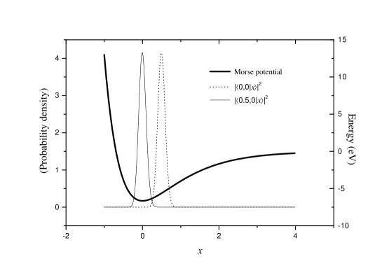
Figure 3.1: The absolute square of the wave functions corresponding to the Morse coherent states $|x_{0},p_{0}=0\rangle$, with $x_{0}=0.0$ (ground state) and $x_{0}=0.5$. These plots correspond to the case of the NO molecule, where $s=54.54$. (We have generated a movie file showing the time evolution of the wave function plotted with dotted line, it can be found in Ref. [10].)

In our calculation we have chosen the NO molecule as our model, where $m=7.46\ {\mathrm{a.u.}}$, $D=6.497\ {\mathrm{eV}}$ and $\alpha=27.68\ {\mathrm{nm^{-1}}}$ [73], yielding $s=54.54$. That is, this molecule has $55$ bound states, and we found that a basis of dimension $N+1=150$ is sufficiently large to handle the problem. The absolute square of the wave functions $|\langle x|0,0\rangle|^{2}$ and $|\langle x|0.5,0\rangle|^{2}$ is depicted in Fig. 3.1, where $V(x)$ is also shown. Fig. 3.1 indicates that initial displacements, $x_{0}$, having the order of magnitude of unity will not lead to “small oscillations”.

The Morse coherent states [71, 74] can be prepared by an appropriate electromagnetic pulse that drives the vibrational state of the molecule starting from the ground state into an approximate coherent state. An example can be found in [77], where the effect of an external sinusoidal field is considered.

3.2 Behavior of expectation values as a function of time

Starting from $|\phi(t=0)\rangle=|x_{0},p_{0}=0\rangle$ as initial states, first we consider the dependence of the $\langle X\rangle(t)$ curve on $x_{0}$.

\psfrag{taxis}{$t/t_{0}$}\psfrag{xlabel}{$\langle X\rangle$}\includegraphics*[bb=45 50 780 520,width=284.52756pt]{fig2.eps}

Figure 3.2: The expectation value of the dimensionless position operator as a function of time. The initial states were $|\phi(t=0)\rangle=|x_{0},p_{0}=0\rangle$, with $x_{0}=1.0$, $x_{0}=0.5$ and $x_{0}=0.06$.

It is not surprising that for small values of $x_{0}$ ($\leq 0.06$) these curves show similar oscillatory behavior as in the case of the harmonic oscillator, see Fig. 3.2. However, when anharmonic effects become important, a different phenomenon can be observed: the amplitude of the oscillations decreases almost to zero, then faster oscillations with small amplitude appear but later we re-obtain almost exactly $\langle X\rangle(0)$, and the whole process starts again. Fig. 3.2 is similar to the collapse and revival in the Jaynes-Cumings (JC) model [78, 79], but in our case the non-equidistant spectrum of the Morse Hamiltonian is responsible for the effect. There are important situations when revivals and fractional revivals [68, 80, 81, 82] of the wave packet can be described analytically [69], but in a realistic model for a diatomic molecule the difficulties introduced by the presence of the continuous spectrum implies choosing an appropriate numerical solution.

The expansion of the initial state in our finite basis $|x_{0},0\rangle=\sum_{n}c_{n}(x_{0})|\psi_{n}\rangle$ shows that for values of $x_{0}$ shown in Fig. 3.2 the maximal $|c_{n}(x_{0})|$ belongs to $n<[s]$. That is, the expectation value

$$\langle X\rangle(t)=\sum_{n,k=0}^{N}c_{n}(x)c_{k}^{*}(x)\langle\psi_{k}|X|\psi_{n}\rangle\exp\left[it{{2\pi}\over{2s+1}}(E_{k}(s)-E_{n}(s))\right]$$ (3.6)

is dominated by the bound part of the spectrum. Damping of the amplitude of the oscillations is due to the destructive interference between the various Bohr frequencies and we observe revival when the exponential terms rephase again.

Quantitatively, we have determined the dominant frequencies in Eq. (3.6) for $x_{0}=0.5$ and found that they fall into two families, see Fig. 3.3.

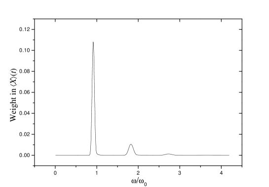
Figure 3.3: The weight of the dominant frequencies responsible for the collapse-revival phenomenon in the expectation value of the position operator. The first peak is related to the matrix elements $\langle\psi_{n}|X|\psi_{n+1}\rangle$, while the second family of nonzero weights corresponds to the matrix elements $\langle\psi_{n}|X|\psi_{n+2}\rangle$.

The first family is related to the matrix elements $\langle\psi_{n}|X|\psi_{n+1}\rangle$ and a has a sharp distribution around $\omega_{1}=0.9\omega_{0}$. The contribution of the second family to the sum in Eq. (3.2) is much weaker, these frequencies around $\omega_{1}=1.81\omega_{0}$ correspond to the matrix elements $\langle\psi_{n}|X|\psi_{n+2}\rangle$. The width the first distribution $\Delta\omega_{1}=0.1\omega_{0}$ allows us to estimate the revival time as $2\pi/\Delta\omega_{1}=62.8t_{0}$, while $\Delta\omega_{2}=0.17\omega_{0}$ is responsible for the partial revival at $t/t_{0}\approx 30$, see Fig 3.2. Following Refs. [68, 80], we denote by $t_{rev}$ the time when the anharmonic terms in the spectrum induce no phase shifts, that is, the initial wave packet is reconstructed. At $t_{rev}/2\approx 60t_{0}$ all these phase factors are $-1$, while $t/t_{0}=30$ corresponds to a quarter-revival, i.e., to time $t_{rev}/4$.

3.3 Time evolution of the Wigner function of the system

In order to gain more insight concerning the physical process leading to the collapse-revival phenomenon seen in Fig. 3.2, one can look at the coordinate representation of the wave function $\phi(x,t)=\langle x|\phi(t)\rangle$. In the representative case of $|\phi(t=0)\rangle=|x_{0},0\rangle$, the wave function is an initially well localized wave packet that gradually falls apart into several packets and then conglomerates again, see Ref. [10].

Starting from the same initial state it is more instructive to visualize the time evolution by the aid of the Wigner function $W(x,p,t)$ that reflects the state of the system in the phase space, see Sec. 2.2.1. The definition given by Eq. (2.13) can be reformulated for a pure state that is represented by its wave function $\phi(x,t)$, yielding

$$W(x,p,t)={{1}\over{2\pi}}\int_{-\infty}^{\infty}\phi^{*}(x+u/2,t)\phi(x-u/2,t)e^{iup}du.$$ (3.7)

Fig. 3.4 a) shows the initial stage of the time evolution, while Fig. 3.4 b) corresponds to $t/t_{0}=30.$ This second Wigner function is typical for Schrödinger-cat states, compare with Fig. 2.1. $W(x,p)$ in Fig. 3.4 b) corresponds to a superposition of two states that are well-localized in both momentum and coordinate, and represented by the two positive hills centered at $x_{1}=-0.1$, $p_{1}=-18.0$ and $x_{2}=0.3$, $p_{2}=12.0$. The strong oscillations between them shows the quantum interference of these states.

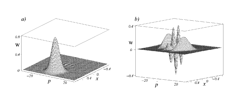
Figure 3.4: Wigner functions of the Morse system at the initial stage of the time evolution and the formation of a Schrödinger-cat state. The plots a) and b) correspond to $t/t_{0}=0$ and $t/t_{0}=30$, respectively. The initial state was $|\phi(t=0)\rangle=|x_{0},p_{0}=0\rangle$, with $x_{0}=0.5$. (The movie file showing the time evolution of $W$ can be found in Ref. [10].)

According to the our calculations, there are a few periods around $t/t_{0}=30$, while the state of the system can be considered to be a phase space Schrödinger-cat state. During this time the Wigner function is similar to the one shown in Fig. 3.4 b), and it rotates around the equilibrium position. Similar behavior of the Wigner function was found in [83] for the JC model. This effect is responsible for the partial revival around $t/t_{0}=30$ shown in Fig. 3.2, where the frequency of the oscillations is twice that of the oscillations around $t=0$: in the neighborhood of $t/t_{0}=30$ there are two wave packets moving approximately the same way as the coherent state soon after $t=0$.

3.4 Measuring nonclassicality

According to Sec. 2.2.1, the Wigner function of a state $|\phi\rangle$ can be used to determine the nonclassicality of $|\phi\rangle$. Having calculated $W(x,p)$, it is straightforward to obtain the quantity $0\leq M_{nc}<1$ (defined by Eq. (2.18)), which is an appropriate measure of the nonclassicality [63].

\psfrag{tlabel}{$t/t_{0}$}\psfrag{mlabel}{$M_{nc}$}\includegraphics*[bb=50 50 780 520,width=284.52756pt]{fig5.eps}

Figure 3.5: Nonclassicality as a function of time. The initial state was $|\phi(t=0)\rangle=|x_{0},p_{0}=0\rangle$, with $x_{0}=1.0$, $x_{0}=0.5$ and $x_{0}=0.06$.

Fig. 3.5 shows $M_{nc}$ as a function of time for the same initial states as in Fig. 3.2. For the small initial displacement of $x_{0}=0.06$, we see that the Wigner function is positive almost everywhere, the state can be considered as a classical one during the whole time evolution.

For larger initial displacements we can easily identify two time scales. The shorter one is the period of the wave packet in the potential, while the second time scale can be identified with the revival time. Looking at the initial part of the curve $M_{nc}(t)$, we observe that the state of the system is the most classical at those turning points where $\langle X\rangle>0$, see Fig. 3.1. On the other time scale, the collapse of the oscillations in $\langle X\rangle$ presents itself as the increase of $M_{nc}$, and the revival turns the state into a more classical one. When the state of the system can be considered as a Schrödinger-cat state, $M_{nc}(t)$ has a small local minimum, but it still has significant values indicating strong nonclassicality.

3.5 Conclusions

We have found that in the potential of the NO molecule, when anharmonic effects are important, the time evolution naturally leads to the formation of Schrödinger-cat states at certain stages of the time evolution. These highly nonclassical states correspond to the superposition of two molecular states which are well localized in the phase space.

Chapter 4 Decoherence of molecular wave packets

The correspondence between classical and quantum dynamics of anharmonic systems has gained significant attention in the past few years [68, 80, 70, 69]. A short laser pulse impinging on an atom or a molecule excites a superposition of several stationary states, and the resulting wave packet follows the orbit of the corresponding classical particle in the initial stage of the time evolution. However, the nonequidistant nature of the involved energy spectra causes peculiar quantum effects, broadening of the initially well localized wave packets, revivals and partial revivals [80, 68, 70, 69, 81, 82]. As we saw in the previous chapter, partial revivals are in close connection with the formation of Schrödinger-cat states, which, in this context, are coherent superpositions of two spatially separated, well localized wave packets [84]. Phase space description of vibrational Schrödinger-cat state formation using animated Wigner functions can be found in [10]. According to Chap. 1, these highly nonclassical states are expected to be particularly sensitive to decoherence. The aim of this chapter is to analyze the process of decoherence for the spontaneously formed Schrödinger-cat states in the anharmonic Morse potential.

In the following we introduce a master equation that takes into account the fact that in a general anharmonic system the relaxation rate of each energy eigenstate is different. This master equation is applied to the case of wave packet motion in the Morse potential that is often used to describe a vibrating diatomic molecule. Considering the phase space description of decoherence, we show how the phase portrait of the system reflects the damping of revivals in the expectation values of the position and momentum operators due to the effect of the environment. We also calculate and plot the time evolution of the Wigner function corresponding to the reduced density operator of the Morse system. The Wigner function picture visualizes the fact that although our master equation reduces to the amplitude damping equation (2.19) in the harmonic limit, the anharmonic effects lead to a decoherence scheme which is similar to the phase relaxation (see Sec. 2.2.2 and also Ref. [45]) of the harmonic oscillator (HO). It is found that the time scale of decoherence is much shorter than that of dissipation, and gives rise to density operators which are mixtures of localized states along the phase space orbit of the corresponding classical particle. We illustrate the generality of this decoherence scheme by presenting the time evolution of an energy eigenstate as well. We also calculate the decoherence time for various initial wave packets. We show that decoherence is faster for wave packets that correspond to a classical particle with a phase space orbit of larger diameter.

4.1 A master equation describing decoherence in the Morse system

We consider a vibrating diatomic molecule and recall the Morse Hamiltonian

$$H_{S}=P^{2}+(s+1/2)^{2}[\exp(-2X)-2\exp(-X)],$$ (4.1)

which is often used to describe this system, see Sec. 3.1. The initial wave packets of our analysis – similarly to the previous chapter – will be Morse coherent states [71], $|x_{0},p_{0}\rangle$, which are localized on the phase space around the point $(x_{0},p_{0})$, see Fig. 3.4. Although the construction given in [72] would allow us to use arbitrary initial states, for our current purpose it suffices to consider states $|x_{0},p_{0}\rangle$ with negligible dissociation probability, i.e., coherent states that practically can be expanded in terms of the bound states $|\phi_{n}\rangle$, $n=0,1,\ldots[s]$. This means that the relevant part of the spectrum of $H_{S}$ is nondegenerate and discrete.

The environment is assumed to consist of the modes of the free electromagnetic field

$$H_{E}=\sum_{k}\hbar\omega_{k}(a^{\dagger}_{k}a_{k}+1/2).$$ (4.2)

We assume the following interaction Hamiltonian

$$V=\hbar\mathcal{X}^{\dagger}\sum_{k}g_{k}a_{k}+\hbar\mathcal{X}\sum_{k}g_{k}a^{\dagger}_{k},$$ (4.3)

where, for the sake of simplicity, the coupling constants $g_{k}$ were taken to be real. Wishing to keep the derivation as general as it is possible, the only necessary restriction on the operator $\mathcal{X}$ is that it must have a strictly upper triangular matrix in the eigenbasis $\{|\phi_{n}\rangle\}$, i.e., $\mathcal{X}$ transforms each eigenstate of $H_{S}$ into a superposition of different eigenstates corresponding to lower energy values. $\mathcal{X}^{\dagger}$ is the Hermitian conjugate of $\mathcal{X}$. This is the application of the rotating wave approximation (RWA) to an anharmonic, multilevel system. Well-known examples imply that from the viewpoint of decoherence RWA is a permissible approximation. According to Ref. [51], in the case of spontaneous emission, RWA on the initial Hamiltonian modifies the level shifts induced by the environment. This could be expected, because the total Hamiltonian with and without RWA has usually different spectra. However, the damping term that provides the time scale of the spontaneous emission is practically unaffected by keeping the counter rotating terms in the interaction Hamiltonian. A similar result was found for the case of a spin-${{1}\over{2}}$ system in external magnetic field [85] and also for a single two-level atom in electric field [86].

Note that in the particular case of a vibrating diatomic molecule, the operators $\mathcal{X}$ and $\mathcal{X}^{\dagger}$ gain a clear interpretation: in the eigenbasis of Morse Hamiltonian $H_{S}$, they are the upper and lower triangular parts of the molecular dipole moment operator, $\hat{\mu}$. We will assume that $\hat{\mu}$ is linear [87], that is, proportional to the displacement $X$ of the center of mass of the diatomic system from the equilibrium position. Although in this chapter the resulting master equation will be applied to describe the decoherence of a vibrating diatomic molecule, we do not perform the $X\rightarrow$ $\mathcal{X}$ substitution during the derivation in order to indicate the generality of our approach.

Using the specific operators above, we can return to Eq. (2.12)

$${{d}\over{dt}}\rho_{S}^{i}(\tau)=-{{1}\over{\hbar^{2}}}\int_{0}^{\tau}dt_{1}{\mathrm{Tr}}_{E}\left[V^{i}(\tau),\left[V^{i}(t_{1}),\rho_{S}^{i}(\tau)\rho^{i}_{E}(0)\right]\right],$$ (4.4)

and perform the integration in order to obtain a differential equation that describes the time evolution of the reduced density matrix of our system, $\rho_{S}$. The interaction picture operator $V^{i}$ is defined by Eq. (2.5), and its expansion in the eigenbasis $\{|\phi_{n}\rangle\}$ of the system Hamiltonian has the form

$$V^{i}(t)=\sum_{m>n}e^{{{i(E_{m}-E_{n})t}\over{\hbar}}}\mathcal{X}^{\dagger}_{mn}|\phi_{m}\rangle\langle\phi_{n}|\ \sum_{k}e^{{-i\omega_{k}t}}g_{k}a_{k}+h.c.,$$ (4.5)

where we invoked that $\mathcal{X}_{mn}^{\dagger}=0$ if $m\leq n$. $E_{0}$ denotes the ground state energy, and the eigenvalues of $H_{S}$ follow each other in increasing order: $E_{m}>E_{n}$, whenever $m>n$. Therefore the integrand in Eq. (4.4) contains $16$ terms. However, by assuming that the environment is in thermal equilibrium at a given temperature $T$, we can deduce that the terms containing $\sum_{k,l}g_{k}g_{l}\ a^{\dagger}_{k}a^{\dagger}_{l}$ and its adjoint give no contribution, because ${\mathrm{Tr}}_{E}[a^{\dagger}_{k}a^{\dagger}_{l}\rho_{E}]=0$. (We note that for some specially prepared reservoirs, such as squeezed reservoirs, this quantity need not be zero, see [55].) Moreover, since

$${\mathrm{Tr}}_{E}\left(a^{\dagger}_{k}a_{l}\ \rho_{E}\right)=\delta_{kl}\langle a^{\dagger}_{k}a_{k}\rangle_{\rho_{E}}\ \ \ {\textnormal{and}}\ \ \ \ {\mathrm{Tr}}_{E}\left(a_{k}a^{\dagger}_{l}\ \rho_{E}\right)=\delta_{kl}\langle a_{k}a_{k}^{\dagger}\rangle_{\rho_{E}},$$ (4.6)

we have

$${\mathrm{Tr}}_{E}\sum_{k,l}g_{k}g_{l}\ a^{\dagger}_{k}a_{l}\ \rho_{E}=\sum_{k}(g_{k})^{2}\overline{n}_{k},\ \ \ \ \ \textrm{and}\ \ \ \ \ {\mathrm{Tr}}_{E}\sum_{k,l}g_{k}g_{l}\ a_{k}a_{l}^{\dagger}\ \rho_{E}=\sum_{k}(g_{k})^{2}\left(\overline{n}_{k}+1\right),$$ (4.7)

where $\overline{n}_{m}=\langle a^{\dagger}_{m}a_{m}\rangle_{\rho_{E}}=1/(\exp(\frac{\hbar\omega_{m}}{kT})-1)$ is the average number of quanta in the $m$-th mode of the environment. According to the assumption that the environment consists of a large number of harmonic oscillators, we can convert the sum over modes to frequency-space integral $\int_{0}^{\infty}d\omega D(\omega)\ldots$, where $D(\omega)$ denotes the density of states which is proportional to $\omega^{2}$ in our case. The continuous version of Eq. (4.7) combined with Eq. (4.4) yields to

$${{d}\over{dt}}\rho_{S}(\tau)=-\int_{0}^{\tau}dt_{1}\int_{0}^{\infty}d\omega D(\omega)g^{2}(\omega)$$

$$\times \Big{[}\mathcal{X}(\tau)\mathcal{X}^{\dagger}(t_{1})\rho_{S}(\tau)\overline{n}(\omega)e^{{-i(t_{1}-\tau)\omega}}+\mathcal{X}^{\dagger}(\tau)\mathcal{X}(t_{1})\rho_{S}(\tau)\left(\overline{n}(\omega)+1\right)e^{{i(t_{1}-\tau)\omega}}$$

$$- \mathcal{X}^{\dagger}(\tau)\rho_{S}(\tau)\mathcal{X}(t_{1})\left(\overline{n}(\omega)+1\right)e^{{i(t_{1}-\tau)\omega}}-\mathcal{X}(\tau)\rho_{S}(\tau)\mathcal{X}^{\dagger}(t_{1})\overline{n}(\omega)e^{{-i(t_{1}-\tau)\omega}}+\mathrm{h.c.}\Big{]},$$

where the superscript $i$ referring to the interaction picture was omitted. Choosing the first term as a representative example, the application of Eq. (4.5) leads to

$$I_{1}=\int_{0}^{\tau}\!\!dt_{1}\!\!\int_{0}^{\infty}\!\!d\omega D(\omega)g^{2}(\omega)\mathcal{X}(\tau)\mathcal{X}^{\dagger}(t_{1})\rho_{S}(\tau)\overline{n}(\omega)e^{{-i(t_{1}-\tau)\omega}}$$

$$= \!\!\!\!\!\!\sum_{l,m<l,n<l}\!\!\!\!\mathcal{X}_{ml}\mathcal{X}^{\dagger}_{ln}e^{{{i(E_{m}-E_{n})\tau}\over{\hbar}}}|\phi_{m}\rangle\langle\phi_{n}|\ \rho_{S}(\tau)\int_{0}^{\tau}\!\!\!\!dt_{1}\!\!\int_{0}^{\infty}\!\!d\omega D(\omega)g^{2}(\omega)\overline{n}(\omega)e^{{-i(t_{1}-\tau)(\omega-\omega_{l}+\omega_{n})}},$$

(4.9)

where $\omega_{m}=E_{m}/\hbar$ and $\omega_{l}=E_{l}/\hbar$. Interchanging the order of the time and frequency integral and introducing the variables $t_{2}=\tau-t_{1}$, $\omega_{ln}=\omega_{l}-\omega_{n}>0$ we obtain

$$I_{1}=\sum_{l,m<l,n<l}\mathcal{X}_{ml}\mathcal{X}^{\dagger}_{ln}e^{{{i(E_{m}-E_{n})\tau}\over{\hbar}}}|\phi_{m}\rangle\langle\phi_{n}|\ \rho(\tau)\int_{0}^{\infty}d\omega\int^{\tau}_{0}dt_{2}D(\omega)g^{2}(\omega)\overline{n}(\omega)e^{{it_{2}(\omega-\omega_{ln})}}.$$ (4.10)

At this point it is worth recalling that $\tau$ is the duration of a time interval which is short from the system’s point of view, i.e., the interaction picture reduced density operator changes a little during $\tau$. However, since the interaction is assumed to be weak, the relation $\tau\gg 1/\omega_{ln}$ also holds. This allows us to extend the upper limit of the time integration to infinity in Eq. (4.10). Then the identity

$$\int_{0}^{\infty}du\ e^{\pm iwu}=\pi\delta(w)\pm i{\mathrm{Pv}}\left({{1}\over{w}}\right),$$ (4.11)

where the Dirac-$\delta$ and Cauchy principal value distributions appear on the RHS, allows us to evaluate the integral in $I_{1}$. Eq. (4.11) shows that the effect of the environment is twofold: first it slightly modifies the energy spectrum of the system. This effect is related to the imaginary term in Eq. (4.11). If our aim is not the calculation of the level shifts themselves, then they can be neglected, provided the interaction is not too strong [51]. The second effect of the environment (related to the first term in Eq. (4.11)) is to induce transitions between the (shifted) system energy levels, and this kind of environmental influence is responsible for the decoherence. Therefore we can use the approximation

$$I_{1} \approx \sum_{l,m<l,n<l}\mathcal{X}_{ml}\mathcal{X}^{\dagger}_{ln}e^{{{i(E_{m}-E_{n})\tau}\over{\hbar}}}|\phi_{m}\rangle\langle\phi_{n}|\ \rho(\tau)\int_{0}^{\infty}D(\omega)g^{2}(\omega)\overline{n}(\omega)\pi\delta(\omega-\omega_{ln})$$ (4.12)

$$= U^{\dagger}(\tau)\mathcal{X}\mathcal{X}^{\dagger}_{a}\rho_{S}U(\tau),$$

where we returned to the explicit notation of the interaction picture, and the matrix elements of the operator $\mathcal{X}^{\dagger}_{a}$ are defined by

$$\langle\phi_{m}|\mathcal{X}^{\dagger}_{a}|\phi_{n}\rangle=\langle\phi_{m}|\mathcal{X}^{\dagger}|\phi_{n}\rangle\ \ \pi D(\omega_{nm})g^{2}(\omega_{nm})\overline{n}(\omega_{nm}).$$ (4.13)

The master equation in the Schrödinger picture, neglecting the terms inducing level shifts, reads:

$${{d}\over{dt}}\rho_{S}(\tau) = -{{i}\over{\hbar}}\left[H_{S},\rho_{S}(\tau)\right]-\mathcal{X}^{\dagger}\mathcal{X}_{e}\rho_{S}(\tau)-\mathcal{X}\mathcal{X}_{a}^{\dagger}\rho_{S}(\tau)-\rho_{S}(\tau)\mathcal{X}_{e}^{\dagger}\mathcal{X}-\rho_{S}(\tau)\mathcal{X}_{a}\mathcal{X}^{\dagger}$$ (4.14)

$$+ \mathcal{X}_{a}^{\dagger}\rho_{S}(\tau)\mathcal{X}+\mathcal{X}_{e}\rho_{S}(\tau)\mathcal{X}^{\dagger}+\mathcal{X}^{\dagger}\rho_{S}(\tau)\mathcal{X}_{a}+\mathcal{X}\rho_{S}(\tau)\mathcal{X}^{\dagger}_{e},$$

where each term following the unitary one (the commutator with $H_{S}$) is calculated similarly to $I_{1}$, and

$$\langle\phi_{m}|\mathcal{X}_{e}|\phi_{n}\rangle=\langle\phi_{m}|\mathcal{X}|\phi_{n}\rangle\ \ \pi D(\omega_{nm})g^{2}(\omega_{nm})\left(\overline{n}(\omega_{nm})+1\right).$$ (4.15)

The subscript $e$ here and and $a$ in Eq. (4.13) refers to emission and absorption, respectively. As we can see, the matrix elements (4.13) and (4.15) of the operators that induce the transitions depend on the Bohr frequency of the involved transition, which is a genuine anharmonic feature. In the special case of the HO, when $H_{S}$ has equidistant spectrum, and $\mathcal{X}$ is identified with the usual annihilation operator $a$, both $\mathcal{X}_{a}$ and $\mathcal{X}_{e}$ are proportional to $\mathcal{X}\equiv a$, and Eq. (4.14) reduces to the amplitude damping master equation (2.19) at a finite temperature.

In certain cases one can further simplify Eq. (4.14). When the environment induced relaxation rates are much lower than the relevant Bohr frequencies, the system Hamiltonian induces oscillations that are very fast even on the time scale of decoherence and vanish on the average. Ignoring these fast oscillations we arrive at the interaction picture master equation

$$\frac{d}{dt}\langle\phi_{i}|\rho_{S}|\phi_{j}\rangle=\delta_{i,j}\sum_{k\neq i}\gamma_{ik}\langle\phi_{k}|\rho_{S}|\phi_{k}\rangle-\Gamma_{ji}^{c}\langle\phi_{i}|\rho_{S}|\phi_{j}\rangle,$$ (4.16)

that has already been obtained in Refs. [88, 89] in order to treat the spontaneous emission of a multilevel atom. In Eq. (4.16), $\gamma_{ik}$ denotes a relaxation rate, that is the probability of the $|\phi_{k}\rangle\rightarrow|\phi_{i}\rangle$ transition per unit time, while $\Gamma_{ji}^{c}=1/2\sum_{k}(\gamma_{ik}+\gamma_{jk})$, where

$$\gamma_{ik}=\left\{\begin{aligned} &2\ \langle\phi_{i}|\mathcal{X}_{e}|\phi_{k}\rangle\langle\phi_{i}|\mathcal{X}|\phi_{k}\rangle&&{\textnormal{if}}\ i<k,\\ &0&&{\textnormal{if}}\ i=k,\\ &2\ \langle\phi_{i}|\mathcal{X}_{a}|\phi_{k}\rangle\langle\phi_{i}|\mathcal{X}|\phi_{k}\rangle&&{\textnormal{if}}\ i>k.\end{aligned}\right.$$ (4.17)

However, due to the elimination of the fast oscillations related to $H_{S}$, Eq. (4.16) is not suitable for investigating the wave packet motion and decoherence simultaneously, therefore we propose to use Eq. (4.14). On the other hand we note that Eq. (4.16) radically reduces the computational costs of calculating the time evolution for long times, which might be necessary when the system-environment coupling is very weak.

Supposing that our knowledge is limited to the populations $P_{n}=\langle\phi_{n}|\rho_{s}|\phi_{n}\rangle$, both Eq. (4.14) and Eq. (4.16) leads to the Pauli type equation

$$\frac{d}{dt}P_{n}=\sum_{k}\left(\gamma_{nk}P_{k}-\gamma_{kn}P_{n}\right).$$ (4.18)

Requiring the condition of detailed balance [90] in Eq. (4.18) leads to the steady-state thermal distribution at the temperature of the environment.

In the case of a diatomic molecule in the free electromagnetic field, $g^{2}(\omega)D(\omega)\propto\omega^{3}$, and we assume that $\mathcal{X}=X$, thus the nonzero matrix elements in Eqs. (4.13) and (4.15) are

$$\langle\phi_{m}|\mathcal{X}_{a}|\phi_{n}\rangle =\lambda\ \langle\phi_{m}|X|\phi_{n}\rangle\ {\omega_{nm}}^{3}\ \overline{n}(\omega_{nm}), \ n<m$$ (4.19)

$$\langle\phi_{m}|\mathcal{X}_{e}|\phi_{n}\rangle =\lambda\ \langle\phi_{m}|X|\phi_{n}\rangle\ {\omega_{nm}}^{3}\left(\overline{n}(\omega_{nm})+1\right), \ n>m$$

where the matrix elements of $X$ can be calculated using the algebraic method summarized in [71], and $\lambda=\pi g^{2}(\omega)D(\omega)/\omega^{3}$ is an overall, frequency independent coupling constant. For the sake of definiteness we have chosen the NO molecule as our model.

In order to get insight into the interplay between wave packet motion and decoherence, it is worth considering a stronger molecule-environment interaction than the electromagnetic field modes can provide. Keeping the structure of Eqs. (4.19), this can be done by increasing the value of $\lambda$. Here we present calculations with two different coupling constants, $\lambda_{1}$ and $\lambda_{2}$ which are chosen so that at zero temperature $\omega_{01}/\gamma_{01}\approx 10^{5}$ and $4\times 10^{3}$ for $\lambda=\lambda_{1}$ and $\lambda_{2}$, respectively. This model allows for the numerical integration of the master equation (4.14) (that provides more details of the dynamics than Eq. (4.16)) in a time interval that is long enough to identify the effects of decoherence. These effects can be summarized in a decoherence scheme (see Sec. 4.4) that has a clear physical interpretation, and which is valid also in the weak molecule-environment interaction, when (4.16) is more efficient to calculate the time evolution.

4.2 Time evolution of the expectation values

Starting from $|x_{0},p_{0}=0\rangle$ as initial states, we saw in Chap. 3 that the qualitative behavior of the expectation value $\langle X\rangle(t)=\langle\psi(t)|X|\psi(t)\rangle$ draws the limit of small oscillations. In the absence of environmental coupling (i.e., $\lambda=0$), for $x_{0}\leq 0.06$, $\langle X\rangle(t)$ (as well as $\langle P\rangle(t)$) exhibits sinusoidal oscillations.

\psfrag{plabel}[tl][tl]{$\langle P\rangle$}\psfrag{xlabel}{$\langle X\rangle$}\psfrag{tlabel}{$t/t_{0}$}\includegraphics*[bb=80 50 670 470,width=284.52756pt]{fig6.eps}

Figure 4.1: Phase portrait corresponding to the time evolution of the initial state $|\psi(t=0)\rangle=|x_{0},p_{0}=0\rangle$, with $x_{0}=0.5$. The parameters are $\lambda=\lambda_{1}$, $T=5\ \hbar\omega_{01}/k$, and $t_{0}$ is the period of the small oscillations in the potential. The initial point $\langle X\rangle=0.5$, $\langle P\rangle=0$ together with the starting direction is also indicated.

For larger initial displacements from the equilibrium position, the anharmonic effects become apparent. The collapse and revival in $\langle X\rangle(t)$ and $\langle P\rangle(t)$ can be explained by referring to the various Bohr frequencies that determine their time dependence: dephasing of these frequencies leads to the collapse of the expectation value, and we observe revival when they rephase again.

For the initial state of $|x_{0},0\rangle$, with $x_{0}=0.5$, the original phase of the eigenstates is restored [68, 80] around the full revival time $t_{rev}=110\ t_{0}$, where $t_{0}$ is the period of the small oscillations in the potential. At $t/t_{0}=55$ and $t/t_{0}=27.5$ half and quarter revivals [68, 80] can be observed. Fig. 4.1 shows the damping of the revivals both in $\langle X\rangle(t)$ and $\langle P\rangle(t)$ when interaction with the environment is turned on. Note that the phase portrait of the corresponding classical particle would be a helix with monotonically decreasing diameter, revivals are of quantum nature. However, Fig. 4.1 does not provide a complete description of the time evolution in the phase space, this can be given by using Wigner functions, see Sec. 4.4.

4.3 Decoherence times

Our master equation (4.14) describes decoherence as well as dissipation. However, the time scale of these processes is generally very different, providing a useful tool to distinguish the stages of the time evolution that are dominated either by decoherence or dissipation [8].

\psfrag{elabel}[tl][tl][0.8]{$S(t)$}\psfrag{trlabel}[bl][bl][0.8]{$\mathrm{Tr}\left[\rho_{S}^{2}(t)\right]$}\psfrag{eaxis}{$S$}\psfrag{traxis}[br][bl]{$\mathrm{Tr}\rho_{S}^{2}$}\psfrag{taxis}{$t/t_{0}$}\includegraphics*[bb=65 45 775 515,width=284.52756pt]{fig7.eps}

Figure 4.2: The entropy and the purity of the reduced density matrix of the Morse system as a function of time, calculated using Eq. (4.14). The coupling parameter (see Sec. 4.1) is $\lambda=\lambda_{1}$ and $T=10\ \hbar\omega_{01}/k$. The initial state was $|\psi(t=0)\rangle=|x_{0},0\rangle$, with $x_{0}=2.0$.

In Fig. 4.2 an example is depicted showing how the method of time scale separation works. We have calculated the entropy

$$S=-\mathrm{Tr}\left[\rho_{S}\ln(\rho_{S})\right],$$ (4.20)

as well as the quantity $\mathrm{Tr}[\rho_{S}^{2}]$, which measures the purity of the reduced density operator. Note that the $\mathrm{Tr}$ operation without subscript refers to the trace in the system’s Hilbert space. Decoherence time $t_{d}$ is defined as the time instant that divides the time axis into two parts where the character of the physical process is clearly different. Initially both $S(t)$ and $\mathrm{Tr}[\rho_{S}^{2}(t)]$ change rapidly but having passed $t_{d}$ (emphasized by a vertical line in Fig. 4.2), the moduli of their derivative significantly decrease. After $t_{d}$ the entropy and the purity change on the time scale which is characteristic of the dissipation of the system’s energy during the whole process. The time dependence of the participation ratio $K$ given by Eq. (1.9) is found to be similar to that of the entropy and purity. We note that the typical value of $K$ at the decoherence time was around $5$, that is, just a few modes of the environment were active. The same surprising result was found in Ref. [40], in the context of spontaneous emission from a two-level atom.

In summary, decoherence dominated time evolution turns into dissipation dominated dynamics around $t_{d}$. In the next section we shall determine the density operators into which the process of decoherence drives the system. In connection with these results we have verified that the states around the decoherence time do not change appreciably in a time interval that covers the possible errors in determining $t_{d}$.

An interesting question is the dependence of the decoherence time on the initial state of the time evolution. We calculated $t_{d}$ as a function of the initial displacement for the case of displaced ground states (that is, coherent states with zero momentum, $|x_{0},0\rangle$) as initial states. It was found that for all values of $\lambda$ and $T$, the decoherence time is longer for smaller initial displacements. Additionally, for fixed $\lambda$ and $T$ the function $t_{d}(x_{0})$ can be well approximated by an exponential curve $t_{d}(x_{0})=t_{d}(0)\exp(-\kappa x_{0})$. E. g., for $\lambda=\lambda_{1}$, $T=10\ \hbar\omega_{01}/k$ and $0<x_{0}\leq 2$ the parameters take the values $t_{d}(0)=93\ t_{0}$ and $\kappa=0.97$.

It is known (see Chap. 3 and Ref. [80]) that quarter revivals in an anharmonic potential lead to the formation of Schrödinger-cat states, i.e., states that are superpositions of two distinct states localized in space [80] as well as in momentum [10, 91]. On the other hand, smaller initial displacements correspond to classical phase space orbits with smaller diameter. Consequently the quantum interference related to nonclassical states that are formed during the course of time cover a smaller area in the phase space in this case. This means that our result is a manifestation of the general feature of decoherence that increasing the “parameter of nonclassicality”, which is the diameter of the corresponding classical orbit in our case, causes faster decoherence [27]. A similar result was found in [8] for the case of decoherence in a system of two-level atoms [63, 92].

4.4 Wigner function description of the decoherence

In order to visualize the time evolution of the reduced density matrix of the Morse system we have chosen the Wigner function picture, which has been summarized in Sec. 2.2.1. This description allows us to investigate the correspondence between classical and quantum dynamics.

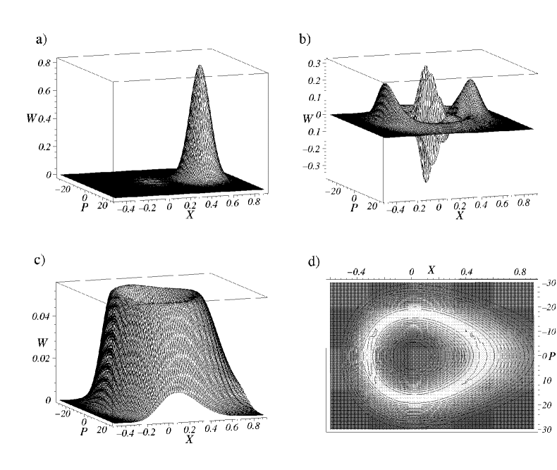
Figure 4.3: Time evolution of the Wigner function corresponding to the initial state $|\psi(t=0)\rangle=|x_{0},0\rangle$, with $x_{0}=0.5$. The coupling parameter is (see Sec. 4.1) $\lambda=\lambda_{2}$ and $T=0.3\ \hbar\omega_{01}/k$. The plots a) and b) correspond to time instants $t/t_{0}=0\ \text{and}\ 27.5$, while both c) and the contour plot d) are snapshots taken at $t/t_{0}=137.5$.

First we recall the ideal case without environment. Then, in the initial stage of the time evolution, the positive hill corresponding to the wave packet $|x_{0},p_{0}\rangle$ follows the orbit of the classical particle that has started from $(x_{0},p_{0})$ at $t=0$. However, due to the uncertainty relation, the Wigner function as a quasiprobability distribution has a finite width, and this fact combined with the form of the Morse potential implies the stretching of the Wigner function along the classical orbit in the course of time. (See Ref. [91] for similar results with the Husimi $Q$ function.) After a certain time the increasingly broadened wave packet becomes able to interfere with itself, and around the quarter revival time one can observe two positive hills chasing each other at the opposite sides of the classical orbit. The strong oscillations of $W$ between the hills represent the quantum correlation of the constituents of this molecular Schrödinger-cat state [84]. Later on the initial Wigner function is restored almost exactly and Schrödinger-cat state formation starts again. Detailed Wigner function description of these processes that are related to the free time evolution can be found in [10].

In the case when environmental effects are present, we found that decoherence follows a general scheme. A representative series of Wigner functions is shown in Fig. 4.3. The snapshots correspond to the initial state and time instants when the first and third Schrödinger-cat state formation would occur in the absence of the environment. Consequently, the Wigner function in Fig. 4.3 b) corresponds almost to a Schrödinger-cat state, but this state is already a mixture. However, there are still negative parts of the function in between the positive hills centered at $x_{1}=0.51,\ p_{1}=0$ and $x_{2}=-0.34,\ p_{2}=0$. The “ridge” that connects these hills along the classical orbit is absent in a pure Schrödinger-cat state, see Fig. 3.4 b). Later on this ridge becomes more and more pronounced and at the decoherence time we arrive at the positive (that is, classical in the sense of Sec. 2.2.1) Wigner function of Fig. 4.3 c) and d). According to the contour plot Fig. 4.3 d), the highest values of this function trace out the phase space orbit of the corresponding classical particle. That is, $\rho_{S}^{dec}$, the reduced density matrix that arises as a result of decoherence, can be interpreted as a mixture of localized states that are equally distributed along the orbit of the corresponding classical phase space orbit.

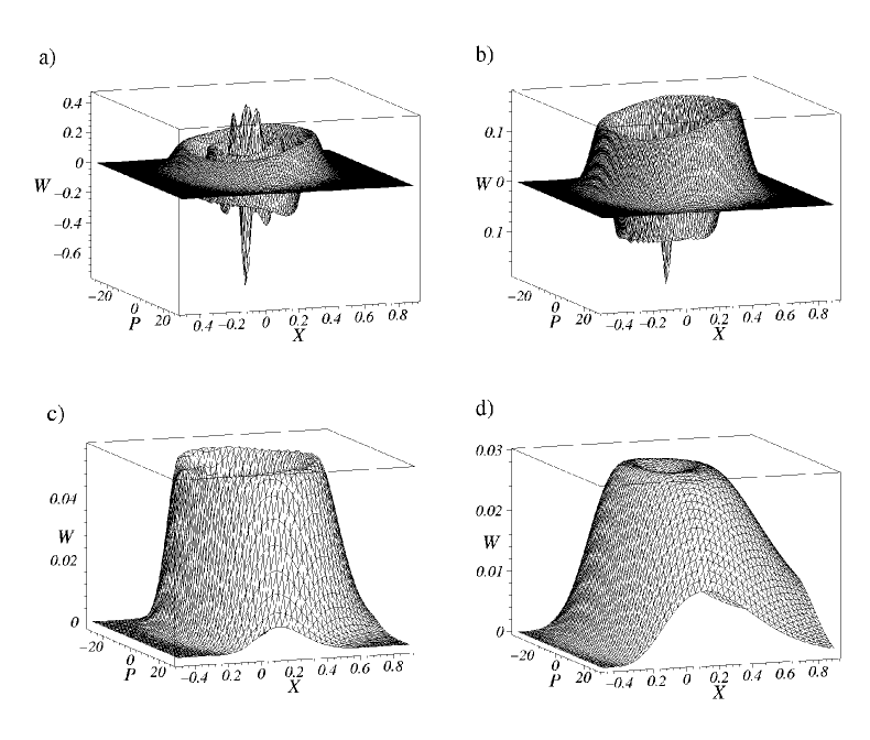
Figure 4.4: Time evolution of the Wigner function corresponding to the fifth bound state as initial state. The coupling parameter (see Sec. 4.1) is $\lambda=\lambda_{1}$ and $T=10\ \hbar\omega_{01}/k$. The plots a), b), c) and d) correspond to time instants $t/t_{0}=0,\ 27.5,\ 330$ and $1000$, respectively.

It is worth comparing this result with the case of the HO, when the master equation (4.14) reduces to the amplitude damping equation (2.19), see Sec. 2.2.2. It is known that harmonic oscillator coherent states are robust against the decoherence described by the amplitude damping master equation (as well as against the Caldeira-Leggett [19] master equation [46]), the initial superposition of coherent states turns into the statistical mixture of essentially the same states. This is a consequence of the facts that these states are eigenstates of the destruction operator $a$, and the operators in the nonunitary terms of Eq. (4.14) are proportional to $a$ and $a^{\dagger}$ in the harmonic case. None of these statements can be transferred to the anharmonic system, where the Morse coherent states do not remain localized during the course of time, even without environment. Therefore the scheme of the decoherence is qualitatively different for the harmonic and anharmonic oscillators: Our results in the anharmonic system are similar to the phase relaxation in the harmonic case [45], where the energy of the system remains unchanged, but the phase information is completely destroyed, see Sec. 2.2.2. We note that a similar result was obtained in Ref. [93], where the rotational degrees of freedom were considered as a reservoir for the harmonic vibration of hot alkaline dimers.

Our decoherence scheme is universal to a large extent. In the investigated domain of the coupling constants $\lambda_{1}\leq\lambda\leq\lambda_{2}$ and temperatures ranging from $T=0$ to $T=15\ \hbar\omega_{01}/k$, it is found to be valid for all initial states, not only for coherent states. Fig. 4.4 shows an example when the initial state is not a wave packet, it is the fifth bound state, corresponding to $E_{5}$, which is very close to $\langle 0.5,0|H_{S}|0.5,0\rangle$, so direct comparison with Fig. 4.3 is possible. As we can see, although the two Wigner functions are initially obviously very different, they follow different routes (that takes different times) to the same state: Fig. 4.3 c) and Fig. 4.4 c) are practically identical. The final plot in Fig. 4.4 indicates how the Wigner function represents the long way to thermal equilibrium with the environment: the distribution becomes wider and the hole in the middle disappears.

It is expected that the loss of phase information has observable consequences. According to the Franck-Condon principle, the absorption spectrum of a molecule around the frequency corresponding to an electronic transition between two electronic surfaces depends on the vibrational state. The time dependence of the spectrum should exhibit the differences between the pure state of an oscillating wave packet and the state $\rho_{S}^{dec}$ and the thermal state. More sophisticated experimental methods based on the detection of fluorescence [94] or fluorescence intensity fluctuations [95], surely have the capacity of observing the dephasing phenomenon considered in this chapter.

4.5 Conclusions

We investigated the decoherence of wave packets in the Morse potential. The decoherence time for various initial states was calculated and it was found that the larger is the diameter of the phase space orbit described by a wave packet, the faster is the decoherence. We obtained a general decoherence scheme, which has a clear physical interpretation: The reduced density operator that is the result of the decoherence is a mixture of states localized along the corresponding classical phase space orbit.

Chapter 5 A system of two-level atoms in interaction with the environment

Two-level atoms are essential objects in quantum optics, several important models rely on this notion [78, 79, 51, 49, 50]. Clearly, most atoms have much more than two energy levels, i.e., considering only two of them is a simplification. However, in usual (experimental) situations the initial conditions and the frequency of the external electromagnetic field or the long lifetime of the lower level supports the two-level view of the atomic system. Additionally, a two-level atom provides a physical realization of a qubit, which is the basic entity in quantum computation (QC)[5, 96, 97].

In the present chapter we investigate a system which is a candidate for the experimental study of decoherence and possibly also for practical applications. The model consists of several identical two-level atoms (the system) interacting with a large number of photon modes in a thermal state (the environment). It has the advantage that it is simple to make the correct transition from a microscopic system to a macroscopic one by increasing the number of atoms. We point out how the master equation (4.14) reduces to the equation appropriate in this case [98, 51, 99], and use it to analyze the evolution of the reduced density matrix of the atomic system.

By analytical short-time calculations we show that the atomic coherent states [14] of our system are robust against decoherence caused by the realistic interaction we consider. The possibility of classical interpretation and this behavior justifies that the superpositions of atomic coherent states are relevant with respect to the original problem of Schrödinger, and such a highly nonclassical superposition is rightly called an atomic Schrödinger-cat state [100, 63, 101]. We also note that there are several proposals for the experimental preparation of these type of states [102, 103, 104].

We present the decoherence and dissipation properties of atomic Schrödinger-cat states based on numerical computations of their time evolution. It will be seen that similarly to the case of the Morse system (see Chap. 4), although the one and the same solution of the master equation describes both decoherence and dissipation, the time scales of these processes differ by orders of magnitude. Using this fact, we show how one can make a clear distinction between these two processes despite of the interplay between them, and define the decoherence time. This decoherence time strongly depends on the initial conditions, notably, it is particularly large for a special set of initial cat states [63, 92]. This will be termed as slow decoherence in contrast with the general case which will be referred to as rapid decoherence.

The interplay between decoherence and energy dissipation is the most appreciable in connection with the concept of pointer states that has been summarized in Sec. 1.2. It will be shown that when the decoherence is rapid, then the constituent coherent states of the initial state are pointer states to a very good approximation. However, when there is enough time for dissipation, i.e., when decoherence is slow, then the initial atomic coherent states themselves evolve into mixtures, and therefore a refined scheme of decoherence holds.

In order to underline the contrast between rapid and slow decoherence we superpose four atomic coherent states corresponding to the vertices of a suitably oriented tetrahedron. The time evolution of this four component cat state will be studied by the aid of the spherical Wigner function (Sec. 2.2.1). As it is expected, the interaction with the environment selects that pair from the initial superposition which constitutes a long-lived cat state.

5.1 Description of the model

We consider a system of identical two-level atoms interacting with the environment of macroscopic number of photon modes. With dipole interaction and in the rotating wave approximation the total system is described by the following model Hamiltonian:

$$H=H_{S}+H_{E}+V=\hbar\omega_{\mathrm{a}}J_{z}+\sum_{k}\hbar\omega_{k}a_{k}^{\dagger}a_{k}+\sum_{k}\hbar g_{k}\left(a_{k}^{\dagger}J_{-}+a_{k}J_{+}\right),$$ (5.1)

where $\omega_{\mathrm{a}}$ is the transition frequency between the two atomic energy levels, $\omega_{k}$ denote the frequencies of the modes of the environment and $g_{k}$ are coupling constants. The operators $J_{+}$, $J_{-}$ and $J_{z}$ in the interaction term are dimensionless collective atomic operators obeying the usual angular momentum commutation relations [105]. On replacing $\mathcal{X}^{\dagger}$ and $\mathcal{X}$ by $J_{+}$ and $J_{-}$ respectively, the process we followed in Sec. 4.1 leads to the interaction picture master equation [98, 51]

$$\frac{\rm{d}\rho(t)}{\rm{d}t} = -\frac{\gamma}{2}\ (\overline{n}+1)\ \left(J_{+}J_{-}\rho(t)+\rho(t)J_{+}J_{-}-2J_{-}\rho(t)J_{+}\right)$$ (5.2)

$$-\frac{\gamma}{2}\ \overline{n}\ \left(J_{-}J_{+}\rho(t)+\rho(t)J_{-}J_{+}-2J_{+}\rho(t)J_{-}\right).$$

Here $\overline{n}$ is the mean number of photons in the environment, $\gamma=\pi D(\omega_{a})g^{2}(\omega_{a})$ denotes the damping rate, and for the sake of simplicity the subscript $S$ of the reduced density operator of atomic system has been dropped. Note that the same master equation can be obtained by considering a low-Q cavity containing Rydberg atoms [99].

If the state of the atomic system was initially invariant with respect to the permutations of the atoms, i.e., it was a superposition of the totally symmetric Dicke states [105], the dipole interaction described by $V=\sum_{k}\hbar g_{k}\left(a_{k}^{\dagger}J_{-}+a_{k}J_{+}\right)$ in (5.1) would not destroy this symmetry. Therefore we may restrict our investigation to the totally symmetric $N+1$ dimensional subspace of the whole Hilbert-space of the atomic system. This subspace corresponds to the first column in Fig. 6.1 and it is isomorphic to an angular momentum eigensubspace labeled by $j=N/2$. This model has been proven to be valid in cavity QED experiments with many atoms, as reviewed in [99].

The environment as a static reservoir (represented by the thermal photon modes) continuously interacts with the atomic system influencing its dynamics. As it is obvious, the dissipation of the energy leads to thermal equilibrium in the system, corresponding to the stationary solution of the master equation (5.2). However, as it will be shown here, the same master equation describes also a much more interesting process. The continuous ”monitoring” [17] of the atomic system by the environment results in the total loss of the coherence of the quantum superpositions in the system. This decoherence process is generally extremely fast compared to the dissipation, except for special initial conditions which will be discussed in section 5.3.

5.2 The initial stage of the time evolution

In this section we apply the general concepts introduced in Sec. 1 to our system in order to find the initial states for the master equation (5.2) which are relevant to the original problem of Schrödinger [1, 2] concerning the unobservability of macroscopic superpositions.

First we consider the short-time behavior of the total system. At zero temperature the photon field of the present model is in its pure vacuum state $\left|0\right\rangle$, therefore the initial state factorizes as

$$\left|\Psi(0)\right\rangle=\left|\varphi_{0}(0)\right\rangle\left|0\right\rangle,$$ (5.3)

i.e., there is a single term in the Schmidt decomposition (see Sec. 1) of the compound state. Due to the interaction, this product state evolves into a more general Schmidt sum like Eq. (1.8), or in other words it turns into an entangled state. According to the summary in Sec. 1, the rate of entanglement can be obtained as

$$A=\sum_{k\neq 0,l\neq 0}\left|\left\langle\varphi_{k}(0)\right|\left\langle\Phi_{l}(0)\right|V\left|\varphi_{0}(0)\right\rangle\left|0\right\rangle\right|^{2}.$$ (5.4)

Using the explicit form of the interaction Hamiltonian $V$ in Eq. (5.1), a straightforward calculation leads to

$$A={\cal C}\left(J_{+},J_{-}\right):=\left\langle J_{+}J_{-}\right\rangle-\left\langle J_{+}\right\rangle\left\langle J_{-}\right\rangle,$$ (5.5)

i.e., in our system the rate of entanglement is the normally ordered correlation function of the operators $J_{+}$ and $J_{-}$.

Let us turn to the case of finite temperatures, when the total system has to be represented by a mixed state even at $t=0$. The linear entropy, defined as

$$S_{\mathrm{lin}}={\rm Tr}(\rho-\rho^{2}),$$ (5.6)

can be regarded as a relevant measure of decoherence [27, 26]. Restricting ourselves again to the initial regime of the time evolution, we can make use of the master equation (5.2) and calculate the time derivative of the linear entropy at $t=0$

$$\left(\frac{\partial S_{\mathrm{lin}}}{\partial t}\right)_{t=0}=\gamma\left(\left\langle n\right\rangle{\cal C}\left(J_{-},J_{+}\right)+\left(\left\langle n\right\rangle+1\right){\cal C}\left(J_{+},J_{-}\right)\right).$$ (5.7)

The normally (antinormally) ordered correlation function ${\cal C}\left(J_{+},J_{-}\right)$ (${\cal C}\left(J_{-},J_{+}\right)$), disappears in the eigenstate $\left|j,m=-j\right\rangle$ ($\left|j,m=j\right\rangle$) of $J_{-}$ ($J_{+}$). However, the collective atomic operators $J_{-}$ and $J_{+}$ have no simultaneous eigenstates which would annullate the right hand side of Eq. (5.7). Nevertheless, we are going to show that if the number of atoms $N=j/2$ is large enough, then the correlation functions in Eq. (5.7) are negligible in a class of states called atomic coherent states [14]. These states are labeled by a complex parameter $\tau=\tan(\beta/2)\exp(-i\phi)$ (for the angles $\beta$ and $\phi$ see Fig. 5.1) and can be expanded in terms of the eigenstates of the operator $J_{z}$ (Dicke states) as

$$|\tau\rangle=\sum^{j}_{m=-j}\left(\begin{array}[]{cc}2j\\ j+m\end{array}\right)^{1\over 2}{\tau^{j+m}\over{(1+|\tau|^{2})^{j}}}|j,m\rangle.$$ (5.8)

For large $j$, the atomic coherent states are approximate eigenstates of the operators $J_{-}$ and $J_{+}$ [14, 92]. This statement is understood in the sense that the square of the cosine of the angle $\alpha$ between $\left|\tau\right\rangle$ and $J_{-}\left|\tau\right\rangle$

$$\cos^{2}\alpha={{\left|\left\langle\tau\left|J_{-}\right|\tau\right\rangle\right|^{2}}\over{\left\langle\tau\left|\right.\tau\right\rangle\left\langle\tau\left|J_{+}J_{-}\right|\tau\right\rangle}}$$ (5.9)

differs from unity by a factor which scales as $(j\tau^{2})^{-1}$. Thus $\alpha$ becomes negligible in the $j\to\infty$ limit for finite $\tau$ [92]. The same statement holds for the operator $J_{+}$, therefore both correlation functions in Eq. (5.7) are indeed negligible in the atomic coherent states (5.8).

This suggests that the atomic coherent states are rather stable against the decoherence induced by the photon modes, i.e., they can serve as a model of classical-like macroscopic quantum states. This result is in analogy with the stability of the oscillator coherent states obtained in [26].

Two such states, $\left|\tau_{1}\right\rangle$ and $\left|\tau_{2}\right\rangle$ can be considered as macroscopically distinct, whenever the distance between the parameters $\tau_{1}$ and $\tau_{2}$ is sufficiently large on the complex plane. This implies that the coherent superposition of these states yields an appropriate model of the original paradox of Schrödinger.

Based on these results, the superpositions

$$|\Psi_{12}\rangle={\frac{{|\tau_{1}\rangle+|\tau_{2}\rangle}}{\sqrt{2(1+{\rm{Re}}\;\langle\tau_{1}|\tau_{2}\rangle)}}}$$ (5.10)

will be called atomic Schrödinger cat states [100, 63, 7], see Fig. 5.1. Now we are going to present our results on the decoherence and dissipation dynamics of these type of states.

Figure 5.1: Scheme of an atomic Schrödinger cat state defined by Eq. (5.10). The points labeled by $\tau_{1}$ and $\tau_{2}$ represent the corresponding atomic coherent states on the surface of the Bloch-sphere. The angles defining the parameters $\tau_{1}$ and $\tau_{2}$ are also shown.

5.3 Time scales

A typical result of the numerical integration of Eq. (5.2) is that the time evolution of the states given by Eq. (5.10) can be characterized by two different time scales, as illustrated by Fig. 5.2, where the linear entropy and the energy of the atomic system is plotted versus time.

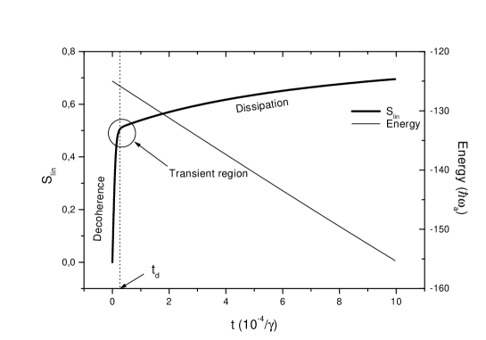
Figure 5.2: The two regimes of the time evolution. (Initially: $\tau_{1}=\tan\pi/4$, $\tau_{2}=0$.) The number of atoms is $N=500$ and the average number of photons is $\overline{n}=1$, $t_{\mathrm{d}}\approx 6\times 10^{-5}/\gamma$

.

As we can see, there exists a time instant $t_{\mathrm{d}}$ (marked with an arrow in Fig. 5.2) when the character of the physical process changes radically. (It is worth comparing this figure with Fig. 4.2, which was obtained in the case of the Morse system.) Initially $S_{\mathrm{lin}}(t)$ increases rapidly while the dissipated energy of the atoms is just a small fraction of that part of the energy which will eventually be transferred to the environment. On the other hand, for longer times $t\gg t_{\mathrm{d}}$ both curves change on the same time scale. The energy of the atomic system decays exponentially as a function of time allowing for identifying the characteristic time of the dissipation, $t_{\mathrm{diss}}$, with the inverse of the exponent. (We note that in Fig. 5.2 the plotted time interval is much shorter than $t_{\mathrm{diss}}$, thus the exponential behavior is not seen.) More detailed calculations have shown that for high temperatures the energy and the linear entropy exhibit similar exponential behavior in the second regime of the time evolution. Their exponents coincide with 2-3% relative error. This implies that the initial stage of the time evolution is dominated by decoherence while after $t_{\mathrm{d}}$ the dissipation determines the dynamics. Accordingly, we define the characteristic time of the decoherence – by the same token as we did in Sec. 4.3 – as the instant when the slope of the curve $S_{\mathrm{lin}}(t)$ decreases appreciably. We note that $t_{\mathrm{d}}$ defined in this way is in accordance with the decoherence time defined previously in [63] for a specific initial state.

It is remarkable that although a few hundred atoms do not really constitute a macroscopic system, the difference of the time scales is obviously seen in Fig. 5.2. It is generally true that the larger $N$ is, the more naturally and sharply the time evolution splits into two regimes.

Now we turn to the investigation of the dependence of the decoherence time $t_{\mathrm{d}}$ on the initial conditions.

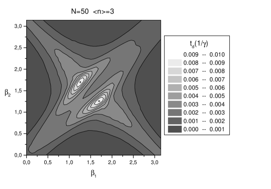
Figure 5.3: The dependence of the characteristic time of the decoherence on the parameters of the initial Schrödinger cat state: $\tau_{1}=\tan\beta_{1}/2$, $\tau_{2}=\tan\beta_{2}/2$. The number of atoms is $N=50$ and the average number of photons is $\overline{n}=3$.

Fig. 5.3 shows the contour plot of the decoherence time versus the parameters $\beta_{1}$ and $\beta_{2}$ (see Fig. 5.1) of the initial atomic Schrödinger cat state (5.10). We have set $\phi_{1}=\phi_{2}=0$ for simplicity. As we can see, the effect of decoherence is remarkably slower when $\beta_{1}\approx\beta_{2}$ which was expected since in this case the overlap of the two initial coherent states is not negligible, so these states can not be considered as “macroscopically distinct”. Much more surprising is the fact that cat states which were initially symmetric with respect to the $(x,y)$ plane (i. e. $\beta_{1}\approx\pi-\beta_{2}$ ) also decohere slower [63, 7], but it is in accordance with the analytical estimations of Braun et.al. [92]. In the following sections we shall refer to these states as symmetric ones.

5.4 The direction of the decoherence

We saw in the previous section that the interplay between decoherence and dissipation is reflected in the time evolution of the superpositions given by Eq. (5.10). In this section we shall focus on the direction of the process resulting from the dynamics governed by the master equation (5.2).

According to Sec. 1, the interaction with a large number of degrees of freedom selects naturally the so-called pointer basis [17] in the Hilbert-space of the system subject to decoherence. This process favors the constituent states of the pointer basis in the sense that the system is driven towards a classical statistical mixture of these states. Thus, from the present point of view $\rho(t_{\mathrm{d}})$ is the relevant quantity to be examined.

Recalling the analytical results of sec. 5.2, it seems plausible to expect that the atomic coherent states (5.8) will be pointer states.

By introducing the density matrix which corresponds to the classical statistical mixture of the initial coherent states:

$$\rho_{\mathrm{cl}}(\tau_{1},\tau_{2})={1\over 2}\left(|\tau_{1}\rangle\langle\tau_{1}|+|\tau_{2}\rangle\langle\tau_{2}|\right),$$ (5.11)

the expected scheme of the decoherence reads:

$$|\Psi_{12}\rangle\langle\Psi_{12}|\rightarrow\rho_{\mathrm{cl}}(\tau_{1},\tau_{2}).$$ (5.12)

We shall refer to $\rho_{\mathrm{cl}}$ as the classical density matrix.

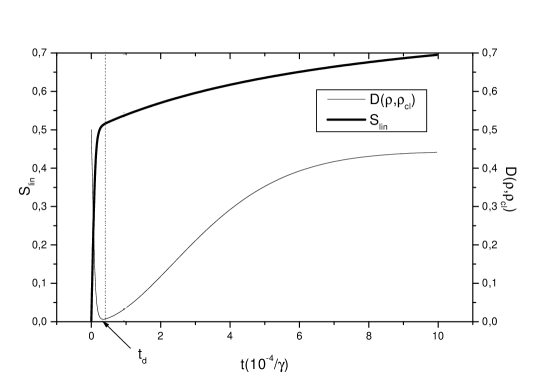
Figure 5.4: The linear entropy $S_{{\mathrm{lin}}}$ and the distance $D$ between $\rho$ and $\rho_{\mathrm{cl}}$ (defined by Eq. (5.13)) in the case of a rapidly decohering Schrödinger cat state ($\tau_{1}=\tan\pi/4$, $\tau_{2}=0$). The number of atoms is $N=500$ and the average number of photons is $\overline{n}=1$.

The distance between the actual density matrix $\rho(t)$ and $\rho_{\mathrm{cl}}$, defined with

$$D\left(\rho(t),\rho_{\mathrm{cl}}\right)={\rm Tr}\left[\left(\rho(t)-\rho_{\mathrm{cl}}\right)^{2}\right],$$ (5.13)

is always decreasing fast. Except for the case of slowly decohering cat states which will be discussed below, $D\left(\rho(t),\rho_{\mathrm{cl}}\right)$ reaches its minimal value at the decoherence time, see Fig. 5.4. This minimal value is very close to zero implying that the density matrix of the system at this instant is nearly the same as the classical density matrix (5.11). This fact justifies the definition of the characteristic time of the decoherence in section 5.3, and it is in excellent agreement with the decoherence scheme (5.12).

Due to the exceptionally slow decoherence, we have to modify this picture if the initial state is a symmetric superposition. In this case the decoherence time is so long that the atomic coherent constituents of the initial state are also appreciably affected by the time evolution until the decoherence time, $t_{d}$. The state of the atomic system at $t_{d}$ will be a mixture, which is the same as if the system had started from $\rho_{\mathrm{cl}}$ at t=0. In other words the evolution follows the modified scheme:

$$|\Psi_{12}\rangle\langle\Psi_{12}|\rightarrow\tilde{\rho}_{\mathrm{cl}}(\tau_{1},\tau_{2},t)$$ (5.14)

where the time dependent classical density matrix $\tilde{\rho}_{\mathrm{cl}}(\tau_{1},\tau_{2},t)$ is the one which would evolve from the statistical mixture (5.11) $\rho_{\mathrm{cl}}(\tau_{1},\tau_{2})=\tilde{\rho}_{\mathrm{cl}}(\tau_{1},\tau_{2},t=0)$ according to the same master equation (5.2) as the actual atomic density matrix. The distance between the time dependent classical density matrix, $\tilde{\rho}_{\mathrm{cl}}$ and $\rho(t)$ becomes negligible at $t_{\mathrm{d}}$, and asymptotically reaches zero for long times in the case of all the initial conditions.

5.5 Wigner functions of four component Schrödinger cat states

The results of the previous section have shown that both the characteristic time and the direction of the decoherence strongly depend on the initial conditions. Now we illustrate this fact by tracking the decoherence of the superposition of four atomic coherent states

$$\left|\Psi_{1234}\right\rangle={\frac{{|\tau_{1}\rangle+|\tau_{2}\rangle+|\tau_{3}\rangle+|\tau_{4}\rangle}}{\sqrt{2(2+{\rm{Re}}\;\sum_{i>k}\langle\tau_{i}|\tau_{k}\rangle)}}}.$$ (5.15)

Since four points on the surface of a sphere are not distinguished with respect to each other if and only if they are the vertices of a regular tetrahedron inscribed in the sphere, we set the components of $\left|\Psi_{1234}\right\rangle$ according to this pattern. On the other hand, the $z$ axis is distinguished in the present model because of the form of the Hamilton operator (5.1), therefore we orient the tetrahedron with one edge parallel to the $z$ axis and the opposite edge parallel to the $y$ axis, see Fig. 5.5. Although we have in principle two substantially different ways of considering the state represented by Fig. 5.5 as the superposition of two atomic Schrödinger-cat states, according to the results of the previous section one expects that the environment naturally selects one of these possibilities via the different time evolutions: the quantum coherence between the components of the symmetric pair $\left|\Psi_{12}\right\rangle\propto\left|\tau_{1}\right\rangle+\left|\tau_{2}\right\rangle$ disappears slowly, while all the other pairs are rapidly decohering superpositions.

Figure 5.5: Phase space scheme of the 4 component cat state. The atomic coherent states constituting the superposition (5.15) are represented by the points labeled by $\tau_{1},\ \ldots,\ \tau_{4}$. They are arranged to form the vertices of a tetrahedron as shown.

We are going to visualize the decoherence process of $\left|\Psi_{1234}\right\rangle$ by the aid of the spherical Wigner function. It is a real function over the unit sphere (which is the appropriate phase space in the present case) being in a linear one-to-one correspondence with the density matrix of the atomic system, see Sec. 2.2.1. For previous applications of this function see [100, 63, 106, 107, 108, 109].

The Wigner function given by Eq. (2.14) suggestively maps the time evolution of the state (5.15) onto the unit sphere, as shown in Fig. 5.6. We plot the Wigner functions of the atomic system at three time instants, both as a polar plot and as a contour plot. Dark shades mean negative, light shades mean positive function values. The four positive lobes, pointing from the center to the vertices of the tetrahedron shown in Fig. 5.5, correspond to the four atomic coherent states in (5.15). Due to the dissipation all these lobes will move slowly downwards. The initial interference pattern (Figs. 5.6 a) and b)) has the regularity of the tetrahedron, there are equally pronounced oscillations along all the edges, representing the quantum coherence between the coherent states.

Figs. 5.6 c) and d) depict the situation after a time which is short in the sense that the the shapes of the lobes of the coherent states are not appreciably affected (no dissipation), but the interference is already negligible between them, except for the single pair along the vertical edge of the tetrahedron. As it is seen from Fig. 5.5 this is the pair which represented initially the symmetric atomic Schrödinger-cat state $\propto\left|\tau_{1}\right\rangle+\left|\tau_{2}\right\rangle$ in (5.15). The coherence between the components of this pair of states is nearly unaffected as shown by the strong oscillations.

A qualitatively different stage of the time evolution is shown in Figs. 5.6 e) and f) at a later time. The coherent constituents are already affected by the dissipation, the uppermost one rather strongly, but the quantum coherence between the components of the symmetric pair is still present. On the contrary, the interference between all the other components has already disappeared.

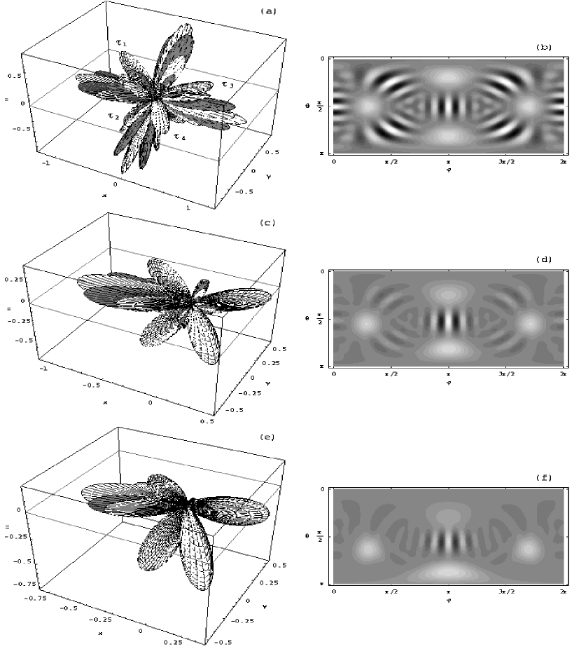
Figure 5.6: Wigner view of the decoherence of the 4 component cat state (5.15). We plot the spherical Wigner function (2.14) both as a polar plot [a), c), e)] and as a contour plot [b), d), f)]. A polar plot is obtained by measuring the absolute value of the function in the corresponding direction, and the resulting surface is shown in light where the values of the Wigner function are positive, and in dark where they are negative. Similarly, light shades of the contour plot correspond to positive function values. Plots a) and b) show the initial state and in a) the lobes corresponding to the initial coherent constituents are also labeled according to Fig. 5.5. Plots c), d) and e), f) show the spherical Wigner function at $t=0.015/\gamma$ and $t=0.04/\gamma$, respectively.

In view of the present results, if the initial state of the atomic system is a superposition of coherent states so that there are symmetric pairs of coherent states in the expansion, then the coherence between the components of these symmetric pairs will survive much longer than between any other terms.

5.6 Conclusions

We have investigated the decoherence of superpositions of macroscopically distinct quantum states in a system of two-level atoms embedded in the environment of thermal photon modes. Utilizing the Schmidt decomposition and the linear entropy, we have shown that atomic coherent states are robust against decoherence, both at zero and non-zero temperatures. This result is in analogy with the harmonic oscillator case and justifies the definition of atomic Schrödinger cat states as superpositions of atomic coherent states.

By solving the master equation (5.2) we have identified two different regimes of the time evolution with the help of the linear entropy. The first one is dominated by decoherence while the second one is governed by dissipation. Based on several computational runs focusing on the characteristic times it was found that $t_{\mathrm{d}}$ decreases much faster than $t_{\mathrm{diss}}$ as the function of the number of atoms, $N$. Consequently $t_{\mathrm{d}}$ becomes many orders of magnitude smaller than the characteristic time of dissipation for macroscopic samples, and even for e.g. $N=500$ atoms and an average photon number of $\overline{n}=1$ the ratio $t_{\mathrm{diss}}/t_{\mathrm{d}}$ is around a few hundred depending on the initial conditions. However, there are very important exceptional cases, called slow decoherence, when the atomic coherent states constituting the initial atomic Schrödinger cat state are symmetric with respect to the equator of the Bloch sphere.

Using a new measure $D$, we have shown that at the characteristic time of decoherence the system is always very close to the state described by the time dependent classical density matrix. Apart from the exceptional case of slow decoherence, the coherent states appearing in (5.10) are approximate pointer states. When due to its symmetry the initial cat state is a long-lived superposition, also its constituent coherent states have time to transform into mixtures until $t_{\mathrm{d}}$. We have given a modified scheme of decoherence which is valid also for slow decoherence.

We have demonstrated the important difference between rapid and slow decoherence by tracking the time evolution of a four component superposition with the help of the spherical Wigner function. The initial interference pattern having the symmetry of a tetrahedron rapidly disappears except for the single slowly decohering pair.

Chapter 6 Preparation of decoherence-free,
subradiant states in a cavity

Decoherence is a difficulty to overcome in the context of QC. Quantum error correction codes [110] offer a possibility for this purpose. A somewhat different approach relies on a specific decoherence-free subspace (DFS) [96, 111, 112]. This idea is essentially a passive error correction scheme: quantum operations are restricted to the DFS in which all the quantum superpositions are much less fragile than in subspaces strongly coupled to the unavoidably present environment.

Subradiant states of a system of two-level atoms [105, 113, 114, 115, 116] has recently gained wide attention because of their exceptionally slow decoherence. This stability of quantum superpositions inside the subradiant subspaces originates from the low probability of photon emission, which means very weak interaction between the atoms and their environment. Hence the subradiant states span a DFS in the atomic Hilbert-space. We note that there are proposals that intend to perform QC within this DFS [112].

Here we propose a scheme that can be used to prepare subradiant states in a cavity. Our method is based on second order perturbation theory but the exact results verify the validity of the perturbative approach [11]. We also investigate to what extent our scheme is independent of the state of the cavity field. The analysis of the conditions shows that this scheme is feasible with present day techniques achieved in atom cavity interaction experiments [117, 28, 118, 119].

6.1 Description of the system

We investigate a system of $N$ identical two-level atoms in a single mode cavity. Each individual atom is equivalent to a spin-$1/2$ system, and the whole atomic ensemble can be described by the aid of collective atomic operators $J_{+}$, $J_{-}$ and $J_{z}$ obeying the same algebra as the usual angular momentum operators[105]. We consider the following model Hamiltonian:

$$H=H_{0}+V=\hbar\omega_{\mathrm{a}}J_{z}+\hbar\omega_{c}a^{\dagger}a+\hbar g\left(a^{\dagger}J_{-}+aJ_{+}\right),$$ (6.1)

where $a$ and $a^{\dagger}$ are the annihilation and creation operators of the cavity mode, $\omega_{\mathrm{a}}$ is the transition frequency between the two atomic energy levels, $\omega_{c}$ denotes the frequency of the cavity mode, different from $\omega_{\mathrm{a}}$, and $g$ is the coupling constant. We note that the Hamiltonian (6.1) is written in the framework of Dicke’s theory, i.e., with the assumption that all the atoms are subjected to the same field, which is a good approximation when the size of the atomic sample is small compared to the wavelength of the cavity mode. As discussed later in detail, there are experimental situations where this requirement is fulfilled. Our proposed scheme for preparing subradiant states involves a detuned cavity. We shall assume that the detuning is much larger than the resonant Rabi frequency:

$$\omega_{c}-\omega_{a}=\Delta\gg g.$$ (6.2)

Now any state of the atomic system and the cavity field can be expanded as a linear combination of the eigenstates of $H_{0}$. These are tensorial products of collective atomic states and number states of the field: $|j,m,\lambda\rangle\otimes|n\rangle$, where the indices $j,m$ and $\lambda$ label the atomic state (also called Dicke state [14]), while $n$ refers to the $n$-th Fock state of the mode.

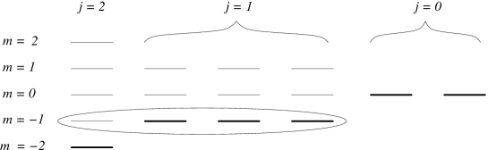
Figure 6.1: Dicke ladders for $N=4$ atoms. Each line corresponds to a collective atomic state, the subradiant states are emphasized by thick lines. The circle denotes the 4-fold degenerate first excited level. The first column corresponds to the completely symmetric subspace.

The quantum number $j$ corresponds to the eigenvalues of the operator $J^{2}=J_{z}^{2}+(J_{+}J_{-}+J_{-}J_{+})/2$. This index is in one-to-one correspondence with the Young diagram [120] that describes the permutation symmetry of the state. The possible values of $j$ are $N/2,N/2-1,\dots$, the smallest value being $0$ if $N$ is even and $1/2$ if $N$ is odd. The index $m$ of the $|j,m,\lambda\rangle$ Dicke state labels the eigenstates of the collective atomic operator $J_{z}$, that is essentially proportional to the energy of the atomic subsystem. This is the index that is decreased (increased) by one under the action of the operator $J_{-}$ ($J_{+}$):

$$J_{-}|j,m,\lambda\rangle=\sqrt{j(j+1)-m(m-1)}|j,m-1,\lambda\rangle,$$ (6.3)

including the case when $m=-j$, when the result is the zero vector. The states with $m=-j$ are the lowest ones of the Dicke ladders [105], they are called subradiant, because they have no dipole coupling to other lower lying states, see Fig. 6.1 for the case of $N=4$. Finally the index $\lambda$ distinguishes states with the same $j$ and $m$. For more details see Refs. [105, 8, 120, 14, 121, 122, 63].

Besides the collective atomic states $|j,m,\lambda\rangle$, we shall also use the natural basis that assigns a well defined state to each individual atom. These vectors will be labeled by a string of $0$-s and $1$-s corresponding to the ground and excited sates, respectively. E. g., the ground state of the atomic subsystem is written in this basis as $|\stackrel{{\scriptstyle 1}}{{0}}\stackrel{{\scriptstyle 2}}{{0}}\ldots\stackrel{{\scriptstyle N}}{{0}}\rangle$; this state (as well as the fully excited one) is also an element of the Dicke basis, $|00\ldots 0\rangle=|j=N/2,m=-N/2,\lambda=1\rangle$.

6.2 Preparation of subradiant states

The form of the Hamiltonian (6.1) implies that the time evolution of the system shall exhibit two time scales: The first characteristic time is due to the self-Hamiltonian $H_{0}$ and is approximately $2\pi/\omega_{a}$ (or $2\pi/\omega_{c}$) and the second is proportional to $2\pi/g$. Generally $g\ll\omega_{a}\approx\omega_{c}$ and the faster process induced by $H_{0}$ can be eliminated by going into an interaction picture. However, if the frequency difference $\Delta$ is large enough, then the energy transfer between two adjacent eigenstates of $H_{0}$, differing in only one photon number, becomes negligible. This means that the amplitude of the corresponding collective Rabi oscillations will be very small, that is, the process on the second time scale will be unnoticeable and even slower mechanisms will become apparent. In this section we are going to show that this situation, which is similar to the one considered in Refs. [123] and [124], gives rise to the preparation of subradiant states.

Hereafter we shall focus on the solution of the Schrödinger equation in the case when just a single atom is excited at $t=0$. This initial state can be prepared by starting from the state $|00\ldots 0\rangle$, and exciting one well defined control atom. This excitation can be achieved via a third much higher lying level, so that the wavelength of the addressing pulse allows to focus it on the desired target atom [125]. For the sake of simplicity we always consider the control atom as being the first, hence the initial state will be written as

$$|\phi(0)\rangle=|100\ldots 0\rangle\otimes|n-1\rangle.$$ (6.4)

In order to find the complete analytical solution of the Schrödinger equation induced by the Hamiltonian (6.1), in principle one should calculate all the eigenvalues and the corresponding eigenstates of $H$. Although this problem can be solved analytically [126], more insight is given by a simple perturbative approach. The exact nonperturbative numerical solution of the Schrödinger equation verifies that results obtained via perturbation theory yield excellent approximations, see section 6.3.

The state

$$|1\rangle\equiv\left({{1}\over{\sqrt{N}}}\sum_{k=1}^{N}|0\ldots 0\stackrel{{\scriptstyle k}}{{1}}0\ldots 0\rangle\right)\otimes|n-1\rangle=$$

$$=|j=N/2,m=-N/2+1,\lambda=1\rangle\otimes|n-1\rangle,$$ (6.5)

which is in the completely symmetric subspace, and the subradiant states:

$$|i\rangle\equiv|j=N/2-1,m=-N/2+1,\lambda=i-1\rangle\otimes|n-1\rangle$$ (6.6)

with $i=2,3...N$, have the same unperturbed energy, they span the $N$-fold degenerate eigensubspace of $H_{0}$ corresponding to the eigenvalue $E^{0}(n)=\hbar(n\omega_{c}-N\omega_{a}/2)-\hbar\Delta$. For the case of $N=4$, the atomic part of the states $|i\rangle$ is denoted by a circle in Fig. 6.1.

It can be seen that first order degenerate perturbation theory is not giving any correction to the energy, because all the matrix elements of $V$ between the states above vanish: The action of $V$ on vectors $|j,m,\lambda\rangle\otimes|n-1\rangle$ gives a linear combination of $|j,m-1,\lambda\rangle\otimes|n\rangle$ and $|j,m+1,\lambda\rangle\otimes|n-2\rangle$ that are orthogonal to the states (6.5) and (6.6). In order to obtain nonzero energy corrections we have to perform a second order degenerate perturbation calculation[127], and find the eigenvalues of the matrix:

$$\sum_{m}{{\langle i|V|m\rangle\langle m|V|k\rangle}\over{E^{0}(n)-E_{m}^{0}}},$$ (6.7)

where the sum runs over all eigenstates of $H_{0}$ with eigenvalue $E_{m}^{0}\neq E^{0}(n)$. The only nonvanishing energy corrections in second order are the following:

$$\delta E_{1} = \hbar{{g^{2}}\over{\Delta}}(Nn-2N-2n+2),$$

$$\delta E_{i} = \delta E_{1}+\hbar N{{g^{2}}\over{\Delta}},\ \ i=2,3\ldots N.$$ (6.8)

At this point we can formulate the requirements that assure the validity of the perturbation theory: the magnitude of $\delta E_{1}$ and $\delta E_{i}$ must be much smaller than $\hbar|\Delta|$, the minimum of the difference between $E^{0}(n)$ and all other unperturbed energy levels.

The most important consequence of Eqs. (6.8) is that the Bohr frequencies that determine the time dependences of the subradiant and non-subradiant states are different.

Now we expand the initial state (6.4) as the linear combination of the fully symmetric (non-subradiant) state $|1\rangle$, and an appropriate subradiant state:

$$|2\rangle={{1}\over{\sqrt{N(N-1)}}}\Big{[}(N-1)|100\ldots 0\rangle-$$

$$\sum_{k=2}^{N}|0\ldots 0\stackrel{{\scriptstyle k}}{{1}}0\ldots 0\rangle\Big{]}\otimes|n-1\rangle.$$ (6.9)

By assigning the symbol $|2\rangle$ to the state in Eq. (6.9), we have utilized the freedom of choosing a basis in the subradiant subspace. Now the initial state reads

$$|\phi(0)\rangle={{1}\over{\sqrt{N}}}|1\rangle+\sqrt{{N-1}\over{N}}|2\rangle.$$ (6.10)

By the aid of this expansion and using the Bohr frequencies resulting from (6.8), it is easy to calculate the time evolution of the state (6.10). Discarding an overall phase factor, this time dependent state has the form

$$|\phi(t)\rangle={{1}\over{\sqrt{N}}}\exp\left(iN{{g^{2}}\over{\Delta}}t\right)|1\rangle+\sqrt{{N-1}\over{N}}|2\rangle,$$ (6.11)

or, on using Eqs. (6.5) and (6.9):

$$|\phi(t)\rangle=\Big{[}\left(N\cos(\alpha t)-i(N-2)\sin(\alpha t)\right)|100\ldots 0\rangle$$

$$+2i\sin(\alpha t)\sum_{k=2}|0\ldots 010\ldots 0\rangle\Big{]}\otimes|n-1\rangle/N.$$ (6.12)

Here we introduced the parameter

$$\alpha={{Ng^{2}}\over{2\Delta}},$$ (6.13)

which is independent of $n$. Because of this latter fact, from now on the state of the cavity field will be omitted in the notation. We also note that the characteristic time of the time evolution, ${{2\pi}/{\alpha}}$, is much longer than that of the free evolution due to $H_{0}$, being the consequence of the fact that the evolution described in Eq. (6.11) is induced by a weak, nonresonant interaction.

Eq. (6.12) reveals that in $|\phi(t)\rangle$ the weight of the state $|100\ldots 0\rangle$ and those of the states with the first atom unexcited changes during the course of time. As we can see, the moduli of the corresponding coefficients in Eq. (6.12) are

$${{\sqrt{N^{2}\cos^{2}(\alpha t)+(N-2)^{2}\sin^{2}(\alpha t)}}\over{N}}\ \ {\rm and}\ \ {{2|\sin(\alpha t)|}\over{N}},$$

respectively. Comparing these values to Eq (6.9), it can be shown that for arbitrary $N$, there exists a time instant $t_{m}$ when

$$|\phi(t)\rangle={{1}\over{\sqrt{N(N-1)}}}\Big{[}(N-1)e^{i\varphi}|100\ldots 0\rangle-$$

$$\sum_{k=2}^{N}|0\ldots 0\stackrel{{\scriptstyle k}}{{1}}0\ldots 0\rangle\Big{]},$$ (6.14)

which differs from the subradiant state $|2\rangle$ only in the phase factor $e^{i\varphi}$ of the first term. Combination of the previous two equations and Eq. (6.9) yields the following requirement for $t_{m}$:

$${{\sqrt{N^{2}\cos^{2}(\alpha t_{m})+(N-2)^{2}\sin^{2}(\alpha t_{m})}}\over{\left|2\sin(\alpha t_{m})\right|}}=N-1.$$ (6.15)

We can find a solution of this equation for all $N>1$:

$$\sin\alpha t_{m}=\sqrt{N/(4N-4)},$$ (6.16)

and also obtain $\cos\varphi={{N-2}\over{2N-2}}$ in Eq. (6.14).

Now it is clear that at the time instant given by Eq (6.16), an appropriate rapid change in the phase of the state $|100\ldots 0\rangle$ relatively to all other states $|0\ldots 0\stackrel{{\scriptstyle k}}{{1}}0\ldots 0\rangle$ leads to the subradiant state $|2\rangle$.

On the other hand, Eq. (6.14) also shows that the required phase transformation is equivalent to the elimination of the phase difference $\varphi$ between the $|1\rangle_{c}$ excited and $|0\rangle_{c}$ ground state of the control atom. Therefore we consider the action of a strong laser pulse on the control atom. In order to obtain precise addressing [125], the laser is to be tuned in resonance with an allowed transition $|1\rangle_{c}\rightarrow|e\rangle_{c}$, where $|e\rangle_{c}$ denotes a state of the control atom with much higher energy than $|1\rangle_{c}$. E. g., by the appropriate choice of the phase of the complex Rabi frequencies of two $\pi$ pulses leads to the phase transformation required to prepare the subradiant state $|2\rangle$. Additionally, the duration of a Rabi period due to the strong, resonant laser pulse is much shorter than the characteristic time that governs the time evolution (6.11). We note that the idea of introducing phase transformation in a multilevel system by the aid of short laser pulses has appeared in a somewhat different context in [128].

Now we show that our scheme is independent of the state of the cavity field, and write more generally the initial state as:

$$|\phi(0)\rangle=|100\ldots 0\rangle\otimes|\psi(t)\rangle=|100\ldots 0\rangle\otimes\sum_{n}c_{n}(t)|n\rangle.$$ (6.17)

We use the fact that the interaction Hamiltonian $V$ does not mix states with different number of excitation (essentially $n+m$):

$$\langle j,m,\lambda|\otimes\langle n|V|n^{\prime}\rangle\otimes|j,m\pm 1,\lambda\rangle=0,$$ (6.18)

unless $n^{\prime}=n\mp 1$. This implies that the calculations based on second order perturbation theory can be performed for each $N$-fold degenerate energy level of $H_{0}$ corresponding to different values of $n$. After replacing the state $|n-1\rangle$ with $|\psi(t)\rangle$ in Eqs. (6.5) and (6.6), we obtain the following result:

$$\delta E_{i}-\delta E_{1}={{g^{2}}\over{\Delta}}N\sum_{n}|c_{n}|^{2}=2\alpha,$$ (6.19)

which is therefore also valid in this general case. Thus we have proven that our scheme does not require special preparation of the cavity field.

6.3 Comparison with experiments

Although the results above can be checked analytically, the scheme is based on second order perturbation theory. Clearly, there are well defined conditions limiting the validity of the perturbative approach and the applicability of this scheme. Now we are going to analyze these conditions in comparison with recent experimental results. As we shall see, present day experimental techniques allow for the preparation of decoherence-free, subradiant states in the proposed way.

The time instants $t_{m}$ (and the whole time evolution) is found to be independent from the cavity field within the framework of our perturbative approach. However, we must require the energy corrections given by Eqs. (6.8) to be much less than $\hbar|\Delta|$, which is the minimal difference between the eigenvalues of $H_{0}$. According to Eqs. (6.8), this can be achieved if the condition

$${\frac{{g}}{{\Delta}}}\sqrt{N}\ll 1$$ (6.20)

holds, and the average number of photons in the cavity field, $\overline{n}$, is not too large. By cooling the apparatus and sending a train of absorbing atoms through the cavity before the experiment takes place [129], average photon numbers $\overline{n}\ll 1$ can be achieved. Therefore until the relation (6.20) holds, the perturbative approach is valid.

In the following we shall compare the requirements of our proposal with the parameters of the atom-cavity experiments of Haroche and co-workers. First of all, as discussed in the review paper [99], the interaction of a number of Rydberg atoms with a single mode cavity is truly described in the framework of the Dicke model. In more recent experiments the time evolution of an entangled state of the cavity field and an atom [28] and also the entangled state of two atoms [129] has been found to be in agreement with theoretical predictions. From our point of view, Ref. [129] is of special interest, because our proposal is essentially the generalization (with an additional phase transformation) of the two-atom experiment described in that paper to $N$ atoms. In the experiment the atoms emitted by two single atom sources propagate with different velocities and collide inside the cavity. It is possible to apply classical RF pulses on the outgoing atoms independently in order to analyze the final state of the collision process. In our scheme such RF pulses can perform the desired single qubit phase operation and consequently prepare a subradiant state.

In order to investigate the effect of the increasing number of atoms on the applicability of our method we solve numerically the Schrödinger equation induced by the Hamiltonian (6.1) and compare this exact time evolution with the perturbative one. The realistic parameters [28] $g/2\pi\approx 24kHz$ and maximal detunings $\Delta/2\pi\approx 800kHz$ show that the relation (6.20) holds as much as for about hundred atoms. However, it is easy to see that the smallest value of $t_{m}$ increases as the left hand side of Eq. (6.20) decreases, and $t_{m}$ must clearly be shorter than the interaction time which has the order of magnitude of $10\mu s$ [28]. To elucidate the trade-off between this requirement and the validity of the perturbative method, we calculate the minimal $t_{m}$ value for different number of atoms. We use the above realistic value of the coupling constant and choose $\Delta/2\pi=720kHz$, thus $\Delta/g=30$. The resulting graph is shown in Fig. 6.2, where the shortest $t_{m}$ is plotted versus the number of atoms, $N$. In the numerical calculation $t_{m}$ is defined as the time instant when the distance (in the sense of the norm naturally connected to the usual inner product) between the current state and the state given by Eq. (6.14) is minimal.

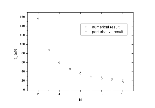
Figure 6.2: The shortest $t_{m}$ values (introduced by Eq. (6.14)) as a function of the number of atoms. Open circles denote the values calculated numerically while crosses correspond to the perturbative approximation, see Eq. (6.16).

With the parameters above the agreement between the numerical and the perturbative results is convincing, this minimal distance is small, less than $0.04$. The validity of the perturbative approach can also be seen by comparing the values of $t_{m}$ obtained in the two different ways.

The most interesting property of Fig. 6.2 is that $t_{m}(N)$ is a decreasing function. This means that once our scheme is implemented with two atoms, the interaction time stipulates no additional conditions on the case of more atoms. Concerning the numerical values appearing in the figure, the conclusion is that the condition $\Delta/g=30$ is too strict in the sense that $t_{m}(2)$ is longer than the interaction time reported in [129]. The effects predicted by perturbation theory can also be observed in the case of a weaker condition. Indeed, based on the agreement of theoretical and experimental results, Ref. [129] draws the limit of the perturbative regime at $\Delta/g>3$.

6.4 Conclusions

We have proposed a method to prepare decoherence-free, subradiant states of a multiatomic system. We also compared the theoretical requirements with the parameters of existing experimental setups and found that the proposed scheme is feasible with presently available experimental techniques.

Summary

The phenomenon that is called decoherence and the correspondence with classical mechanics is a fundamental question in the quantum theory since the 1930s. Nowadays, due to the rapid development of experimental techniques, it is possible to investigate the mechanisms of decoherence also in laboratories. Controlled number of ions in a trap [29, 125], single Rydberg atoms traversing a cavity [129] or EPR pairs of polarized photons [130] can shed new light on long-lived theoretical questions. Besides this principal importance, state of the art experiments in this field offer possibilities for practical applications as well. Quantum cryptography protocols have already been implemented, and there is a hope also for quantum computation to turn into reality. All these facts underline the importance of understanding the role of highly nonclassical quantum states and the process of decoherence in the field of quantum optics.

In this work the focus was on concrete quantum systems, and the related theoretical models were based on the approach of the environment induced decoherence. That is, we assumed that the reason for the emergence of classical properties in a quantum system is the interaction with the environment. An overview of this concept was given in Chap. 1, and Chap. 2 dealt with the mathematical methods that are used to treat open quantum systems. The most important properties of the Wigner functions that are relevant from our point of view have also been given, because these functions are found to visualize decoherence in an instructive way. In Part II of the thesis we presented our own results that are summarized as follows:

Molecular wave packets in an anharmonic potential

The realistic vibrational potential energy of a diatomic molecule in a given electronic state can be approximated by the Morse potential. First we investigated the time evolution of wave packets in this anharmonic potential without the influence of the environment. For small oscillations, the behavior of the wave packets are similar to the harmonic case, but when anharmonicity plays an important role, peculiar quantum effects can be observed. The Wigner function of the system shows that in this case there are certain stages of the time evolution when the vibrational state of the molecule can be considered as a highly nonclassical Schrödinger-cat state: it is the superposition of two other states that are well localized in the phase space.

Decoherence of molecular wave packets

The highly nonclassical Schrödinger-cat states that spontaneously form in the Morse potential provide the motivation for the study of the decoherence in a diatomic molecule. We introduced a model where the environment is represented by a set of harmonic oscillators and took into account that the rate of an environment induced transition depends on the involved Bohr frequencies, which are different for different transitions. This model led to a master equation, the final, steady-state solution of which represents thermal equilibrium with the environment. On the time scale of dissipation decoherence is a very fast process, and the time instant when decoherence dominated time evolution turns into dissipation dominated dynamics, naturally defines the characteristic time of the decoherence. The behavior of the entropy of the molecular system reflects the separation of the two time scales and allows us to determine the decoherence time for different initial wave packets. We found that keeping all other parameters fixed, decoherence becomes faster by increasing the diameter of the a phase space orbit corresponding to the wave packet. It has also been demonstrated that decoherence follows a general scheme in this case, it drives the molecule into the classical mixture of states that are localized along the corresponding classical phase space orbit. This scheme is valid not only for the case of wave packets as initial states, but also for energy eigenstates.

Two-level atoms and decoherence

A system of two-level atoms provides a model in which the microscopic $\rightarrow$ macroscopic (mesoscopic) transition is straightforward: it means the simple increase of the number of the atoms in the ensemble. In this system, starting from superposition of atomic coherent states as initial states, we have shown that the decoherence time can be determined in a way similar to the case of a diatomic molecule: The behavior of the linear entropy changes its character around the decoherence time. The uncertainty of this operational definition decreases when we increase the number of the atoms. We have found that certain superpositions of atomic coherent states, the so-called symmetric Schrödinger-cat states, exhibit exceptionally slow decoherence. We introduced a decoherence scheme that is able to describe the time evolution of these symmetric states as well.

Preparing decoherence-free states

The presence of a cavity around two-level atoms modifies the mode structure of the electromagnetic field surrounding the atoms, and the spontaneous emission rate can be different from that of in free space. The system consisting of the cavity field and the atoms is coupled to the environment also in this case. In order to avoid the decoherence of the atomic state, we introduced a method that can prepare subradiant states in a cavity. These states have recently gained wide attention, because the interaction of the cavity field and the atoms in a subradiant state is negligible, therefore cavity losses do not lead to the decoherence of the atomic state. Therefore the subradiant states span a decoherence-free subspace, which can be important from the viewpoint of quantum computation. Our method for preparing decoherence-free atomic states is based on the natural time evolution of the atomic system in the cavity, and requires the individual manipulation of an initially chosen control atom. The analysis of the experimental requirements of our scheme shows that it can be implemented with present day cavity QED setups.

Bibliography

- [1] E. Schrödinger, Naturwissenschaften 23, 807 (1935).
- [2] E. Schrödinger, Naturwissenschaften 23, 823 (1935).
- [3] O. Hadjar, P. Földi, R. Hoekstra et al., Phys. Rev. Lett. 84, 4076 (2000).
- [4] M. Arndt, O. Nairz, J. Voss-Andreae et al., Nature 401, 680 (1999).
- [5] M. A. Nielsen and I. L. Chuang, Quantum computation and quantum information (Cambridge Univ. Press, Cambridge, 2000).
- [6] P. Földi, M. G. Benedict and A. Czirják, Acta. Phys. Slov. 48, 335 (1998).
- [7] P. Földi, A. Czirják and M. G. Benedict, Acta. Phys. Slov. 50, 285 (2000).
- [8] P. Földi, A. Czirják and M. G. Benedict, Phys. Rev. A 63, 033807 (2001).
- [9] P. Földi, M. G. Benedict and A. Czirják, Fortschr. Phys. 49, 961 (2001).
- [10] P. Földi, A. Czirják, B. Molnár et al., Opt. Express 10, 376 (2002).
- [11] P. Földi, M. G. Benedict and A. Czirják, J. Mod. Opt. 49, 1263 (2002).
- [12] P. Földi, M. G. Benedict and A. Czirják, Phys. Rev. A 65, 021802 (2002).
- [13] P. Földi, M. G. Benedict, A. Czirják et al., Phys. Rev. A 67, Art. No. 032104 (2003), URL quant-ph/0208141.
- [14] F. Arecchi, E. Courtens, R. Gilmore et al., Phys. Rev. A 6, 2221 (1972).
- [15] P. Meystre and M. Sargent, Elements of Quantum Optics (Springer-Verlag, Berlin, Heidelberg, New York, 1991), 2 edn.
- [16] H. D. Zeh, Found. Phys 1, 69 (1970).
- [17] W. H. Zurek, Phys. Rev. D 24, 1516 (1981).
- [18] W. H. Zurek, Phys. Rev. D 26, 1862 (1982).
- [19] A. O. Caldeira and A. J. Leggett, Physica A 121, 587 (1983).
- [20] W. G. Unruh and W. H. Zurek, Phys. Rev. D 40, 1071 (1989).
- [21] B. L. Hu, J. P. Paz and Y. Zhang, Phys. Rev. D 45, 2843 (1992).
- [22] H. Dekker, Phys. Rep. 80, 1 (1981).
- [23] C. M. Savage and D. F. Walls, Phys. Rev. A 32, 2316 (1985).
- [24] L. Diósi, Phys. Rev. A 40, 1165 (1989).
- [25] S. Bose, K. Jacobs and P. L. Knight, Phys. Rev. A 59, 3204 (1999).
- [26] W. H. Zurek, Progr. Theor. Phys 89, 281 (1993).
- [27] D. Giulini, E. Joos, C. Kiefer et al., Decoherence and the Appearance of a Classical World in Quantum Theory (Springer-Verlag, Berlin, Heidelberg, New York, 1996).
- [28] M. Brune, E. Hagley, J. Dreyer et al., Phys. Rev. Lett. 77, 4887 (1996).
- [29] C. J. Myatt, B. King, Q. A. Turchette et al., Nature 403, 269 (2000).
- [30] J. R. Friedman, V. Patel, W. Chen et al., Nature 406, 43 (2000).
- [31] F. Károlyházy, A. Frenkel and B. Lukács, Quantum concepts of space and time, pp. 109–128 (Clarendon Press, 1986).
- [32] R. Penrose, Quantum concepts of space and time, pp. 129–146 (Clarendon Press, 1986).
- [33] J. Ellis, S. Mohanty and D. V. Nanopoulos, Phys. Lett. B 221, 113 (1989).
- [34] J. Neumann, Mathematische Grundlagen der Quantenmechanik (Springer, Berlin, 1932).
- [35] A. Einstein, B. Podolsky and N. Rosen, Phys. Rev. 47, 777 (1935).
- [36] J. S. Bell, Speakable and unspeakable in quantum mechanics (Cambridge University Press, Cambridge, 1987).
- [37] E.Schmidt, Math. Annalen 63, 433 (1907).
- [38] O. Kübler and H. Zeh, Ann. Phys. 76, 405 (1973).
- [39] A. Ekert and P. L. Knight, Am. J. Phys. 63, 415 (1995).
- [40] K. W. Chan, C. K. Law and J. H. Eberly, Phys. Rev. Lett. 88, 100402 (2002).
- [41] M. J. Donald, M. Horodecki and O. Rudolph, The uniqueness theorem for entanglement measures (2001), URL quant-ph/0105017.
- [42] J. Preskill, Quantum information and computation (1998), URL A little effort leads to the correct url ….
- [43] K. Życzkowski, P. Horodecki, A. Sanpera et al., Phys. Rev. A 58, 883 (1998).
- [44] K. Życzkowski, Phys. Rev. A 60, 3496 (1999).
- [45] D. F. Walls and G. J. Milburn, Phys. Rev. A 31, 2403 (1985).
- [46] W. H. Zurek, S. Habib and J. P. Paz, Phys. Rev. Lett. 70, 1187 (1993).
- [47] L. Diósi, Europhys. Lett. 22, 1 (1993).
- [48] C. W. Gardiner, Handbook of Stochastic Methods (Springer-Verlag, Berlin, 1990), 2 edn.
- [49] V. Weisskopf and E. P. Wigner, Z. Physik 63, 54 (1930).
- [50] V. Weisskopf and E. P. Wigner, Z. Physik 65, 18 (1931).
- [51] G. S. Agarwal, Quantum Statistical Theories of Spontaneous Emission and their Relation to Other Approaches, vol. 70 of Springer tracts in modern physics, pp. 1–129 (Springer-Verlag, Berlin, Heidelberg, New York, 1974).
- [52] S. Nakajima, Prog. Theor. Phys. 20, 948 (1958).
- [53] R. Zwanzig, J. Chem. Phys. 33, 1338 (1960).
- [54] R. Zwanzig, Statistical mechanics of irreversibility, vol. 3 of Boulder Lectures in Theoretical Physics, pp. 106–141 (Interscience, 1960).
- [55] D. F. Walls and G. J. Milburn, Quantum Optics (Springer-Verlag, Berlin, 1994).
- [56] C. Cohen-Tannoudji, B. Diu and F. Laloë, Méchanique Quantique, vol. 2 (Hermann, Paris, 1977), 2 edn.
- [57] R. Schack and T. A. Brun, A C++ Library Using Quantum Trajectories to Solve Quantum Master Equations (1996), URL quant-ph/9608004.
- [58] O. Arratia, M. A. Martn and M. A. del Olmo, Deformation in Phase Space (1998), URL math-ph/9805016.
- [59] K. E. Cahill and R. J. Glauber, Phys. Rev. 177, 1882 (1969), ibid. 1882.
- [60] G. S. Agarwal, Phys. Rev. A 24, 2889 (1981).
- [61] R. L. Stratonovich, Sov. Phys. JETP 4, 891 (1957).
- [62] L. C. Biederharn and J. D. Louck, Angular Momentum in Quantum Physics (Addison-Wesley, Reading MA, 1981).
- [63] M. G. Benedict and A. Czirják, Phys. Rev. A 60, 4034 (1999).
- [64] R. J. Glauber, Phys. Rev. 130, 2529 (1963).
- [65] R. J. Glauber, Phys. Rev. 131, 2766 (1963).
- [66] J. Janszky, P. Domokos and P. Adam, Phys. Rev. A 48, 2213 (1993).
- [67] M. Brune, S. Haroche, V. Lefevre et al., Phys. Rev. Lett. 65, 976 (1990).
- [68] J. Parker and C. R. Stroud, Phys. Rev. Lett. 56, 716 (1986).
- [69] D. L. Aronstein and J. C. R. Stroud, Phys. Rev. A 62, 022102/1 (2000).
- [70] S. I. Vetchinkin and V. V. Eryomin, Chem. Phys. Lett. 222, 394 (1994).
- [71] M. G. Benedict and B. Molnár, Phys. Rev. A 60, R1737 (1999).
- [72] B. Molnár, P. Földi, M. G. Benedict et al., Europh. Lett. 61, 445 (2003), URL quant-ph/0202069.
- [73] K. P. Huber and G. Herzberg, Molecular spectra and molecular structure IV. Constants of diatomic molecules (van Nostrand Reinhold, 1979).
- [74] B. Molnár, M. G. Benedict and J. Bertrand, J. Phys. A: Math. Gen. 34, 3139 (2001).
- [75] J. Banerji and G. S. Agarwal, Opt. Exp. 5, 220 (1999).
- [76] J. Bertrand and M. Irac-Astaud, Czech J. Phys. 51, 1272 (2001).
- [77] B. Molnár, M. G. Benedict and P. Földi, Fortschr. Phys. 49, 1053 (2001).
- [78] E. T. Jaynes and F. W. Cummings, Proc. Inst. Elect. Eng. 51, 89 (1963).
- [79] J. H. Eberly, N. B. Narozhny and J. J. Sanchez-Mondragon, Phys. Rev. Lett. 44, 1323 (1980).
- [80] I. S. Averbukh and N. F. Perelman, Phys. Lett. A139, 449 (1989).
- [81] C. Leichtle, I. S. Averbukh and W. P. Schleich, Phys. Rev. A 54, 5299 (1996).
- [82] P. Domokos, T. Kiss, J. Janszky et al., Chem. Phys. Lett. 322, 255 (2000).
- [83] J. Eiselt and H. Risken, Phys. Rev. A 43, 346 (1991).
- [84] J. Janszky, A. V. Vinogradov, T. Kobayashi et al., Phys. Rev. A 50, 1777 (1994).
- [85] F. Bloch and A. Siegert, Phys. Rev. 57, 522 (1940).
- [86] S. H. Autler and C. H. Townes, Phys. Rev. 100, 703 (1955).
- [87] Y.-M. Yuan and W.-K. Liu, Phys. Rev. A 57, 1992 (1998).
- [88] M. Lax, Phys. Rev. 145, 110 (1966).
- [89] G. S. Agarwal, Master Equation methods in quantum optics, vol. XI of Progress in Optics, pp. 3–73 (North Holland, 1973).
- [90] F. Reif, Fundamentals of Statistical and Thermal Physics (McGraw-Hill, Singapore, 1965).
- [91] P. Kasperkovitz and M. Peev, Phys. Rev. Lett. 75, 990 (1995).
- [92] D. Braun, P. A. Braun and F. Haake, Opt. Comm. 179, 411 (2000).
- [93] C. Brif, H. Rabitz, S. Wallentowitz et al., Phys. Rev. A 63, 063404 (2001).
- [94] L. Khundkar and A. H. Zewail, Annu. Rev. Phys. Chem. 41, 15 (1990), and see also references therein.
- [95] C. Warmuth, A. Tortschanoff, F. Milota et al., J. Chem. Phys. 112, 5060 (2000).
- [96] M. B. Plenio, S. F. Huelga, A. Beige et al., Phys. Rev. A 59, 2468 (1999).
- [97] C. H. Bennett and D. DiVincenzo, Nature 404, 247 (2000).
- [98] R. Bonifacio, P. Schwendimann and F. Haake, Phys. Rev. A 4, 302 (1971).
- [99] S. Haroche and J. M. Raimond, vol. 20 of Advances in atomic and molecular physics, pp. 347–411 (1985).
- [100] M. G. Benedict, A. Czirják and C. Benedek, Acta. Phys. Slov. 47, 259 (1997).
- [101] J. Janszky and A. V. Vinogradov, Phys. Rev. Lett. 64, 2771 (1990).
- [102] G. S. Agarwal, R. R. Puri and R. P. Singh, Phys. Rev. A 56, 2249 (1997).
- [103] C. C. Gerry and R. Grobe, Phys. Rev. A 56, 2390 (1997).
- [104] C. C. Gerry and R. Grobe, Phys. Rev. A 57, 2247 (1998).
- [105] R. M. Dicke, Phys. Rev. 93, 439 (1954).
- [106] J. Dowling, G. S. Agarwal and W. P. Schleich, Phys. Rev. A 49, 4101 (1994).
- [107] A. Czirják and M. G. Benedict, Quantum Semiclass. Opt. 8, 975 (1996).
- [108] C. Brif and A. Mann, J. Phys. A: Math. Gen. 31, L9 (1998).
- [109] S. M. Chumakov, A. Frank and K. B. Wolf, Phys. Rev. A 60, 1817 (1999).
- [110] P. W. Shor, Phys. Rev. A 52, 2493 (1995).
- [111] D. A. Lidar, I. L. Chuang and K. B. Whaley, Phys. Rev. Lett. 81, 2494 (1998).
- [112] A. Beige, D. Braun, B. Tregenna et al., Phys. Rev. Lett. 85, 1762 (2000).
- [113] M. G. Benedict, A. M. Ermolaev, V. A. Malyshev et al., Superradiance (IOP, Bristol, 1996).
- [114] M. Gross and S. Haroche, Phys. Rep. 93, 301 (1982).
- [115] D. Pavolini, A. Crubellier, P. Pillet et al., Phys. Rev. Lett. 54, 1917 (1985).
- [116] R. G. DeVoe and R. G. Brewer, Phys. Rev. Lett. 76, 2049 (1996).
- [117] M. Weidinger, B. T. H., Varcoe et al., Phys. Rev. Lett. 82, 3795 (1999).
- [118] E. Hagley, X. Mâitre, G. Nogues et al., Phys. Rev. Lett. 79, 1 (1997).
- [119] A. Rauschenbeutel, G. Nogues, S. Osnaghi et al., Phys. Rev. Lett. 83, 5166 (1999).
- [120] M. Hamermesh, Group Theory and its Applications to Physical Problems (Dover Publications, New York, 1962).
- [121] A. Crubellier and D. Pavolini, J. Phys. B 20, 1451 (1987).
- [122] C. H. Keitel, M. O. Scully and G. Süssmann, Phys. Rev. A 45, 3242 (1992).
- [123] A. Sørensen and K. Mølmer, Phys. Rev. Lett. 82, 1971 (1999).
- [124] S. B. Zheng and G. C. Guo, Phys. Rev. Lett. 85, 2392 (2000).
- [125] H. C. Nägerl, D. Leibfried, H. Rohde et al., Phys. Rev. A 60, 145 (1999).
- [126] M. Tavis and F. W. Cummings, Phys. Rev. 170, 379 (1968).
- [127] L. D. Landau and E. M. Lifshitz, Quantum Mechanics, Nonrelativistic Theory (Pergamon Press, Oxford, 1965).
- [128] G. S. Agarwal, M. O. Scully and H. Walther, Phys. Rev. Lett. 86, 4271 (2001).
- [129] S. Osnaghi, P. Bertet, A. Auffeves et al., Phys. Rev. Lett. 87, 037902 (2001).
- [130] P. G. Kwiat, E. Waks, A. G. White et al., Phys. Rev. A 60, R773 (1999).