Nonlinear interaction of light with Bose-Einstein condensate: new methods to generate subpoissonian light

Abstract

We consider $\Lambda$-type model of the Bose-Einstein condensate of sodium atoms interacting with the light. Coefficients of the Kerr-nonlinearity in the condensate can achieve large and negative values providing the possibility for effective control of group velocity and dispersion of the probe pulse. We find a regime when the observation of the ”slow” and ”fast” light propagating without absorption becomes achievable due to strong nonlinearity. An effective two-level quantum model of the system is derived and studied based on the su(2) polynomial deformation approach. We propose an efficient way for generation of subpoissonian fields in the Bose-Einstein condensate at time-scales much shorter than the characteristic decay time in the system. We show that the quantum properties of the probe pulse can be controlled in BEC by the classical coupling field.

I Introduction

The problem of atom-field interaction represent one of the major areas in the modern physics and quantum optics, particularly Scully and Zubairy (1997); Wolf (2002). A special interest is regarded to effects of propagation of light inside highly nonlinear atomic media where a large nonlinearity is achieved with appropriate choice of the form of the atom-field interaction Imamoglu et al. (1997); Wang et al. (2002). Some early works Basov et al. (1966); Basov and Letokhov (1966) on interaction of a resonance atomic system and laser field demonstrated a possibility to achieve significant difference between phase and group velocity of the light pulses. In the experiments, Letokhov and Basov showed that while the front-edge of the pulse generated the inversion in the system of two-level particles resulted in the sloping of the front-edge, the back process of re-emission of the absorbed energy gave rise to some steeping of the back-edge of the pulse. Hence, the pulse shape deformation resulted in significant delay of its registration on exit from the resonance media that was observed experimentally. The works motivated intensive study of so-called the ”slow” and ”fast” light.

An important step in the development of the theory was the theoretical prediction Garrett and McCumber (1970) and experimental observation Chu and Wong (1982) of positive and negative delays of picosecond pulses propagating without pulse shape deformation inside a crystal. But, very high level of optical losses was limiting the effect to a relatively small magnitude. Basically, there are several different ways to overcome the difficulty. The first idea exploits the shortening of the pulse duration to lengths, which would be much smaller than the relaxation times in the medium that provides necessary conditions for a generation of optical solitons Allen and Ebebley (1978). Another approach is based on a three-level $\Lambda$-scheme. In that case one of two laser beams is a strong coupling field developing a transparency window in the medium and the second probe field propagates through the resonant system without absorption and with unchanged pulse shape Harris et al. (1990).

A sketch of the energy levels in the $\Lambda$-scheme for a single sodium atom is shown in Fig. 1. A classical beam with the central frequency $\omega_{c}$ couples the levels $|1\rangle$ and $|3\rangle$, and the probe pulse with central frequency $\omega_{p}$ couples $|3\rangle$ and $|2\rangle$ levels such that the three levels form a $\Lambda$-type configuration. If the intensities of the classical and probe fields are comparable and the relaxation rates of the levels $|1\rangle$ and $|2\rangle$ are negligible then a state of an atom may be considered as quantum superposition of two lower levels $|1\rangle$ and $|2\rangle$. It corresponds to the effect of so-called coherent trapping of lower states Alzetta et al. (1976); Gray et al. (1978). Another type of dynamics may be realized if the intensity of the probe pulse is much smaller than the intensity of the classical field and the atoms initially populate the lower level $|2\rangle$. The regime is called electromagnetically induced transparency (EIT). In the paper we concentrate on the later.

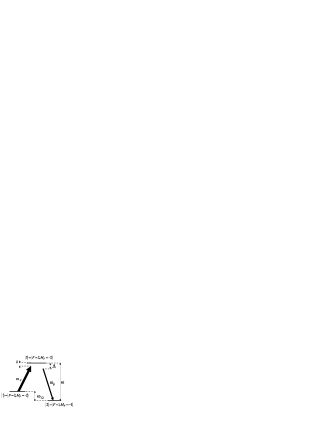
Figure 1: The energy level $\Lambda$-scheme of ${}^{23}Na$ atoms.

Systems in the EIT regime are extensively studied in the literature. Some interesting results are referred to: the studies of the dispersion of the atomic medium in a linear response regime Tewari and Agarwal (1986), semiclassical estimates of the time delay of the probe field inside atomic cells in a thermal equilibrium Harris et al. (1992), EIT in doped crystals Turukhin et al. (2002), nonlinear optical parametric processes in resonant double-$\Lambda$ system Lukin et al. (1998). Wang and colleagues carried out an important experimental measurements of the Kerr nonlinear index of refraction in a three-level Rb atomic $\Lambda$-system using an optical ring-cavity Wang et al. (2001). They found that the Kerr nonlinearity can reach very large and negative values.

One of the dominating problems in EIT was the spectrum broadening regarded to thermal effects. To overcome the difficulty, a highly coherent atomic Bose-Einstein condensate (BEC) is used Ketterle (2002); Cornell and Wieman (2002). Hau and co-workers calculated linear dispersive properties of the system and demonstrated a possibility to observe the ”slow” light effect in the ultra-cold vapor of sodium atoms loaded into a magnetic trap at the temperature of transition to the condensed state Hau et al. (1999). Based on their results we consider EIT effects in the Bose-Einstein condensate of sodium atoms. Two hyperfine sub-levels of sodium state $3^{2}S_{1/2}$ with $F=1,F=2$ are associated with levels $|2\rangle$ and $|1\rangle$ of the $\Lambda$-scheme, correspondingly. An excited state $|3\rangle$ corresponds to the hyperfine sub-level of the term $3^{2}P_{3/2}$ with $F=2$ (see Fig. 1) McClelland and Kelley (1985). The energy splitting between the levels $|1\rangle$ and $|2\rangle$ is denoted by $\omega_{12}/(2\pi)=1772\mathrm{MHz}$, the transition $|3\rangle\rightarrow|2\rangle$ corresponds to the optical frequency $\omega/(2\pi)=5.1\cdot 10^{14}\mathrm{Hz}$ ($\lambda=589\mathrm{nm}$) Mitsunaga et al. (2000).

The condensate is considered being placed inside a confocal resonator. A strong coupling beam propagates along the optical axis of the resonator maintaining the transparency window in the condensate due to the transitions $|1\rangle\rightarrow|3\rangle$. According to the conventional EIT regime the atoms mainly populate the lowest level $|2\rangle$. We assume that the resonator mode has an eigenfrequency $\omega_{c}$. The coupling laser beam develops large polarization in the condensate resulting in significant nonlinear susceptibility of the medium on the frequency $\omega_{p}$. A probe pulse with the appropriately chosen polarization direction propagates transversely to the resonator optical axis. It obeys high nonlinear interaction with the condensate. In order to study a competition between linear and nonlinear processes regarded to the transition $|3\rangle\rightarrow|2\rangle$ induced by the probe pulse, the linear and third order Kerr-like terms in the expansion of atomic susceptibility are considered. An effective control on the absorption of the probe pulse and its group velocity is realized by detuning $\delta$ of the coupling field frequency from the resonance.

In the following section we find conditions when the group velocity of the probe pulse becomes very small or very large. We also note a region where the absorption in the condensate is almost zero what we have called as nonlinear compensation of optical losses. In the third section, the interaction between sodium BEC and the probe pulse is described by an effective quantum Hamiltonian. We explain the way to reformulate linear three level $\Lambda$-scheme in terms of nonlinear quantum model of a two-level particle interacting with quantized field and to solve the model. We apply the su(2) polynomial deformation formalism in order to develop the perturbation theory. In the next section the perturbation theory is considered up to second order. The last fifth section concerns with some nonclassical effects in quantum statistics of the photons in the probe pulse described by the effective Hamiltonian. In the conclusion we discuss some experimental perspectives of our results.

II Nonlinear compensation in sodium BEC.

Applying the formalism of slowly varying field amplitudes Leontovich (1944) in the rotating wave approximation we write the Hamiltonian describing the interaction of three-level atoms with two laser fields in the following form Patnaik et al. (2002):

$$H^{\Lambda}=\omega_{12}|1\rangle\langle 1|+\omega|3\rangle\langle 3|$$

$$-g_{1}|3\rangle\langle 1|e^{-i\omega_{c}(t-\frac{z}{c})}-g_{1}^{*}|1\rangle\langle 3|e^{i\omega_{c}(t-\frac{z}{c})}$$

$$-g_{2}|3\rangle\langle 2|e^{-i\omega_{p}(t-\frac{z}{c})}-g_{2}^{*}|2\rangle\langle 3|e^{i\omega_{p}(t-\frac{z}{c})}.$$ (1)

For simplicity, we let $\hbar=1$ in the paper. In Eq. (II) the coefficients $g_{1,2}$ determine single-photon Rabi frequencies and are defined as follows

$$g_{1}=|\mu_{31}|A_{c},\;g_{2}=|\mu_{32}|A_{p}.$$ (2)

Here, $\mu_{ij}$ is the atomic dipole momentum, $A_{c(p)}$ are the slowly varying coupling and probe field amplitudes, correspondingly.

We denote single-atom density matrix by $\rho=\sum_{\{i,j\}=1}^{3}{\rho_{ij}|i\rangle\langle j|}$. The time evolution of the density matrix is described by the Liouville equation of motion R.Shen (1984)

$$\frac{\partial\rho}{\partial t}=-i\left[{H^{\Lambda},\rho}\right]$$

$$-\gamma_{12}(|1\rangle\langle 1|\rho-2\,|2\rangle\langle 1|\rho|1\rangle\langle 2|+\rho|1\rangle\langle 1|)$$

$$-\gamma_{32}(|3\rangle\langle 3|\rho-2\,|2\rangle\langle 3|\rho|3\rangle\langle 2|+\rho|3\rangle\langle 3|)$$

$$-\gamma_{31}(|3\rangle\langle 3|\rho-2\,|1\rangle\langle 3|\rho|3\rangle\langle 1|+\rho|3\rangle\langle 3|).$$ (3)

Here, the constants $\gamma_{ij}$ determine the rate of spontaneous decay from the levels $|i\rangle$ to $|j\rangle$ in the $\Lambda$-scheme. In general, to consider the space-time dynamics of the system of fields and atoms interacting in the resonator we have to add to Eq. (II) the Maxwell equations

$$\bigtriangledown\times\bigtriangledown\times\vec{\mathbf{E}}=-\frac{1}{c^{2}}\frac{\partial^{2}\vec{\mathbf{E}}}{\partial t^{2}}-\frac{1}{\varepsilon_{0}c^{2}}\frac{\partial^{2}\vec{\mathbf{P}}}{\partial t^{2}}.$$ (IIa)

Here, $c$ is the velocity of light in the vacuum, $\vec{\mathbf{E}}$ is the total amplitude of corresponding fields. The vector $\vec{\mathbf{P}}$ is the polarization of the condensate induced by the coupling or probe field, correspondingly.

In the adiabatic limit, when the variation of the Rabi frequency $g_{1}$ is very small Lukin and Imamog?lu (2000) a self-consistent problem of Eqs. (II) and (a) may be reduced to a less complicated one. In that case the system of equationscan be solved separately for the medium and the fields. Averaged the density matrix elements over the rapidly oscillating phase of the fields we represent $\rho$ in the following form

$$\rho_{ii}=\bar{\rho}_{ii},\;\rho_{31}=\bar{\rho}_{31}e^{-i\omega_{c}(t-\frac{z}{c})},\;\rho_{32}=\bar{\rho}_{32}e^{-i\omega_{p}(t-\frac{z}{c})},$$

$$\rho_{12}=\bar{\rho}_{12}e^{-i(\omega_{p}-\omega_{c})(t-\frac{z}{c})},$$ (4)

together with the relation $\bar{\rho}_{ij}=\bar{\rho}_{ji}^{*}$. A bar in the matrix elements $\bar{\rho}$ denotes the averaged quantities. Substituting definitions Eq. (II) into Eq. (II) one obtains equations of motion for $\bar{\rho}$ matrix elements

$$\dot{\bar{\rho}}_{11}=-ig_{1}\bar{\rho}_{13}+ig_{1}^{*}\bar{\rho}_{31}-2\gamma_{12}\bar{\rho}_{11}+2\gamma_{31}\bar{\rho}_{33},$$

$$\dot{\bar{\rho}}_{22}=-ig_{2}\bar{\rho}_{23}+ig_{2}^{*}\bar{\rho}_{32}+2\gamma_{12}\bar{\rho}_{11}+2\gamma_{32}\bar{\rho}_{33},$$

$$\dot{\bar{\rho}}_{33}=ig_{1}\bar{\rho}_{13}-ig_{1}^{*}\bar{\rho}_{31}+ig_{2}\bar{\rho}_{23}-ig_{2}^{*}\bar{\rho}_{32}-2(\gamma_{32}+\gamma_{31})\bar{\rho}_{33},$$

$$\dot{\bar{\rho}}_{21}=-i(\delta-\Delta)\bar{\rho}_{21}-ig_{1}\bar{\rho}_{23}+ig_{2}^{*}\bar{\rho}_{31}-\gamma_{12}\bar{\rho}_{21},$$ (5)

$$\dot{\bar{\rho}}_{31}=-i\delta\bar{\rho}_{31}+ig_{1}(\bar{\rho}_{11}-\bar{\rho}_{33})+ig_{2}\bar{\rho}_{21}$$

$$-(\gamma_{12}+\gamma_{32}+\gamma_{31})\bar{\rho}_{31},$$

$$\dot{\bar{\rho}}_{32}=-i\Delta\bar{\rho}_{32}+ig_{2}(\bar{\rho}_{22}-\bar{\rho}_{33})+ig_{1}\bar{\rho}_{12}-(\gamma_{32}+\gamma_{31})\bar{\rho}_{32}.$$

Here, $\Delta=\omega-\omega_{p}$ and $\delta=\omega-\omega_{12}-\omega_{c}$.

Since we are interested in nonlinear interaction of the BEC with the probe pulse in the dipole approximation we only consider the explicit dependence of $\bar{\rho}_{32}$ on the Rabi frequency $g_{2}$ of the probe field,

$$\bar{\rho}_{32}=\bar{\rho}_{32}^{(0)}+\bar{\rho}_{32}^{(1)}g_{2}+\bar{\rho}_{32}^{(2)}|g_{2}|^{2}+\bar{\rho}_{32}^{(3)}|g_{2}|^{2}g_{2},$$ (6)

where $\bar{\rho}_{32}^{(0)}=0$ denotes initial polarization in the condensate, which is zero for the sodium. The coefficient $\bar{\rho}_{32}^{(1)}$ corresponds to the stationary solution of the system Eq. (II) in the linear approximation and it is responsible for the linear susceptibility of the medium. The nonlinear corrections $\bar{\rho}_{32}^{(2)}$ and $\bar{\rho}_{32}^{(3)}$ determine resonant nonlinear atomic susceptibility. The calculation shows that $\bar{\rho}_{32}^{(2)}$ it is negligible comparing with the Kerr type nonlinearity $\bar{\rho}_{32}^{(3)}$, Hence, we neglect the second order correction $\bar{\rho}_{32}^{(2)}$ in the paper.

We study the dynamics of $|2\rangle$ and $|3\rangle$ levels of sodium atoms interacting with the probe field. We characterize the transition $|2\rangle\rightarrow|3\rangle$ in terms of the effective coupling constant associated with the dipole matrix element $\bar{\rho}_{32}$. Considering all atoms being initially in the state $|2\rangle$, i.e. $\bar{\rho}_{22}=1,\bar{\rho}_{11}=\bar{\rho}_{33}=0$ we find from Eq. (II)

$$\bar{\rho}_{32}^{(1)}=\frac{1}{\Gamma},\;\bar{\rho}_{32}^{(3)}=\frac{i}{\Gamma}\frac{\Gamma^{*}-\Gamma}{2|\Gamma|^{2}}\left({\frac{1}{2\gamma_{opt}}+\frac{1}{\gamma_{mag}}}\right),\;$$ (7)

where

$$\Gamma=\Delta-i2\gamma_{opt}+\frac{|g_{1}|^{2}}{i\gamma_{mag}-\Delta},$$ (8)

$$\gamma_{opt}=\frac{\gamma_{32}+\gamma_{31}}{2},\;\gamma_{mag}=\gamma_{12}.$$ (9)

A total polarization vector of the BEC coupled to the probe electromagnetic field is given in the form $\vec{\mathbf{P}}=\vec{\mathbf{P}}^{(l)}+\vec{\mathbf{P}}^{(nl)}$ Agrawal (2001). Here $\vec{\mathbf{P}}^{(l)}=\epsilon_{0}\hat{\chi}^{(1)}\cdot\vec{\mathbf{E}}$ describes the linear contribution, and

$$\vec{\mathbf{P}}^{(nl)}=\epsilon_{0}\left({\hat{\chi}^{(2)}:\vec{\mathbf{E}}\vec{\mathbf{E}}+\hat{\chi}^{(3)}:\vec{\mathbf{E}}\vec{\mathbf{E}}\vec{\mathbf{E}}+\ldots}\right)$$ (10)

is the nonlinear response on the external fields. The hat denotes tensors. Using well-known relation for the polarization induced in a resonance medium $\vec{\mathbf{P}}=\frac{\cal N}{V}\mu_{32}\bar{\rho}_{32}$ Wolf (2002) and Eq. (7) we find first and third order nonlinear susceptibilities of the Bose-Einstein condensate:

$$\chi^{(1)}=\frac{\cal N}{V}\frac{|\mu_{32}|^{2}}{\epsilon_{0}\Gamma},$$

$$\chi^{(3)}=i\frac{2{\cal N}}{3V}\frac{|\mu_{32}|^{4}}{\epsilon_{0}}\frac{\Gamma^{*}-\Gamma}{\Gamma|\Gamma|^{2}}\left({\frac{1}{2\gamma_{opt}}+\frac{1}{\gamma_{mag}}}\right).$$ (11)

Here ${\cal N}$ is a number of atoms in BEC, $V$ is the volume, and ${\cal N}/V$ is the density of the condensate. Earlier, a similar form for the linear susceptibility $\chi^{(1)}$ of BEC in the EIT regime was obtained in the paper Hau et al. (1999). The nonlinear part $\chi^{(3)}$ of Kerr type was studied in the regime of giant nonlinearities induced in a cyclic process of $\Lambda$-type interaction between optical fields and ”hot” ${}^{87}\mathrm{Rb}$ atoms in atomic cells inside an optical ring cavity Wang et al. (2001).

The permittivity of Bose gas corresponding to the probe field and including linear and nonlinear terms, reads Agrawal (2001)

$$\epsilon_{p}=1+\chi^{(1)}+\frac{3}{4}\chi^{(3)}|A_{p}|^{2}.$$ (12)

Hence, using the relation $\epsilon_{p}=\left({n_{p}+i\frac{\eta_{p}c}{2\omega_{p}}}\right)^{2}$ and Eq. (II) we find the refraction index $n_{p}$ and the absorption coefficient $\eta_{p}$ in first order with respect to the intensity of the probe field

$$n_{p}=n_{p}^{(0)}+n_{p}^{(2)}|A_{p}|^{2},\;n_{p}^{(0)}=1+\frac{1}{2}\mathrm{Re}(\chi^{(1)}),$$

$$n_{p}^{(2)}=\frac{3}{8}\mathrm{Re}(\chi^{(3)});$$ (13)

$$\eta_{p}=\eta_{p}^{(0)}+\eta_{p}^{(2)}|A_{p}|^{2},\;\eta_{p}^{(0)}=\frac{\omega_{p}}{c}\mathrm{Im}(\chi^{(1)}),$$

$$\eta_{p}^{(2)}=\frac{3\omega_{p}}{4c}\mathrm{Im}(\chi^{(3)}).$$ (14)

In the work, the Bose-Einstein condensate is described by the $\Lambda$-scheme in near to resonance regime. The concentration of sodium atoms in the condensate ${\cal N}/V=3.3\cdot 10^{12}\mathrm{cm^{-3}}$ is taken from Hau et al. (1999) and the coupling field intensity $I_{c}=55\mathrm{\frac{mW}{cm^{2}}}$. Taking the dipole matrix element $|\mu_{32}|=22\cdot 10^{-30}\mathrm{C\cdot m}$ from Al-Awfi and Babiker (2000) and making use of the definition $A_{c}=\sqrt{\frac{2I_{c}}{c\epsilon_{0}}}$ Agrawal (2001) we calculate the coupling constant ${g_{1}}/(2\pi)=21.4\mathrm{MHz}$. The probe pulse is assumed to have a time-length of $1\mathrm{\mu s}$, the laser waist inside the BEC is $d=3.7\mathrm{\mu m}$. The intensity of the probe pulse $I_{p}=80\mathrm{\frac{\mu W}{cm^{2}}}$ corresponds to 25 photons in average.

Due to atomic coherence in BEC, in absence of the Doppler broadening the decay rates $\gamma_{31}$ and $\gamma_{32}$ of the level $|3\rangle$ can be estimated by natural (spontaneous) width of transitions from the upper levels of sodium atoms. Taken from the paper Al-Awfi and Babiker (2000) the lifetime on the upper level is $T_{rel}=16.3\mathrm{ns}$, so we assume $\gamma_{32}/2\pi=\gamma_{31}/2\pi=5\mathrm{MHz}$. The decay rates of transitions between the hyperfine levels $|1\rangle$ and $|2\rangle$ is ${\gamma_{12}}/({2\pi})=38\mathrm{KHz}$ according to Wolf (2002).

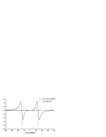
Figure 2: The refraction index $n_{p}^{(2)}$ and the absorption coefficient $\eta_{p}^{(2)}$ of ${}^{23}\mathrm{Na}$ BEC as functions of the detuning $\frac{\Delta}{2\pi}$.

In Fig. 2 we plot a typical frequency dependence of the nonlinear optical refraction index and absorption coefficient as functions of detuning $\Delta$. Giant nonlinear refraction index formed in the condensate with appropriately chosen detuning of the probe pulse is exploited in the paper to demonstrate the possibility of generating subpoissonian statistics of photons on very short time-scales. It is also worth noticing that the realization of a negative $n_{p}^{(2)}$ is similar to the effects observed in Wang et al. (2001), and it may have some important physical applications.

On the other hand, the alternation of regions with positive and negative absorption coefficient corresponds to the regimes of effective nonlinear reduction or amplification of the probe field intensity in the BEC. In both cases, the energy is transformed between the coupling field and the probe pulse. The case of zero absorption $\eta_{p}=0$ may be characterized as a nonlinear EIT. Notice that the regime of complete absence of optical losses in the system falls at the region of very large values of $n_{p}$. It opens even more extensive perspectives to generate nonclassical light in the system. In generally, varying the intensity of the coupling and probe light, and the detuning $\Delta$ we can control the parameter $\Gamma$ in Eq. (II) and change linear and nonlinear relative impact on the probe pulse in the condensate.

Figure 3: The group refraction index $n_{g}$ as a function of the detuning $\frac{\Delta}{2\pi}$.

To understand the effect of ”slow” light in the system we study a frequency dependence of some characteristics of the probe pulse envelope. In Fig. 3 we plotted the group refraction index $n_{g}=n_{p}+\omega_{p}\frac{dn_{p}}{d\omega_{p}}$. A point $\Delta=0$ of the exact resonance corresponds to the EIT regime Harris et al. (1990) characterized by low losses and large $n_{g}$. Under chosen resonance conditions, the group velocity $v_{g}=c/n_{g}$ is $2000m/s$ while the losses are $\eta_{p}=242m^{-1}$. So, the regime corresponds to the effect of ”slow” light. An interesting point in Fig. 3 is a zero of the group refraction index $n_{g}$ that indicates an uncertainty of the group velocity $v_{g}$ of the probe pulse. The uncertainty depicts a possibility to observe superluminal velocities. This effect together with the negative group refraction index is explained in the literature Garrett and McCumber (1970); Mitchell and Chiao (1997) by the presence of plane waves of different frequencies, which appear in the medium long before the pulse peak enters into it. When the group velocity is negative ($n_{g}<0$) the pulse generates two anti-propagating pulses in the BEC. One of them propagates backward (negative velocity) and prevents the peak from traveling forward in the medium.

In the following sections we concentrate on some effects in dynamics of the weak probe pulse. These effects are induced in the system of highly correlated three-level particles by relatively strong classical coupling field. We show how the later can control some quantum properties of the probe pulse.

III The effective two-level quantum model

We are interested in quantum properties of the probe field and define the field in terms of creation and annihilation operators $a^{\dagger},a$. Considering only two levels $|2\rangle$ and $|3\rangle$ of interest for the dynamics of the probe field we work in the EIT limit, i.e. most of the atoms is concentrated on the lower level $|2\rangle$. We assume that the classical field is strong and describe its influence in terms of effective coupling constant for the probe field. The effective two-level Hamiltonian in dipole and rotating-waves approximations reads

$$H=\omega_{p}(a^{\dagger}a+S_{3}+\frac{\cal N}{2})+\Delta S_{3}+k_{1}(aS_{+}+a^{\dagger}S_{-})$$

$$+k_{2}(a^{\dagger}aa^{\dagger}S_{-}+aa^{\dagger}aS_{+}).$$ (15)

The operators $S_{\pm},S_{3}$ describe total dipole momentum corresponding to the transitions $|3\rangle\leftrightarrow|2\rangle$ for the atoms in BEC. The first and the second terms give the free energy of the probe field and atoms. The third term describes linear contribution into the interaction between the field and two-level particles in dipole approximation. It has the typical form of so called the Tavis-Cummings Tavis and Cummings (1968) or Dicke model Dicke (1954). The last term in Eq. (III) describes nonlinear processes due to the presence of strong classical coupling field, and it depends on the intensity of the probe pulse. Both coupling constants are defined below.

An interaction between the BEC and the probe field is determined by the effective matrix element of atomic dipole momentum between $|2\rangle$ and $|3\rangle$ levels. Due to induced nonlinearity the matrix element depends on the intensity of the probe field described by the operator $a^{\dagger}a$ and on the intensity of the coupling field given by a c-number parameter. We define overall coupling constant in the dipole approximation as follows

$$k_{0}\frac{\bar{\rho}_{32}(g_{1},\Delta,g_{2})}{\bar{\rho}_{32}^{(1)}(g_{1}=0,\Delta)g_{2}},$$ (16)

where $\bar{\rho}_{32}$ is given in Eq. (6), and $k_{0}=\mu_{32}\sqrt{\frac{\omega}{2\hbar\varepsilon_{0}V}}$ is the single-photon Rabi-frequency in the Dicke modelAndre and Lukin (1954). The form-factor in Eq.(16) satisfies the condition that at zero coupling field it approaches unity. This behavior of the form-factor results from the fact that when $g_{1}\approx 0$ the induced nonlinearity for the probe field should vanish.

From the definition Eq.(16) and the expansion of $\bar{\rho}_{32}$ in Eqs. (6), (7) we find the coupling constants $k_{1}$ and $k_{2}$

$$k_{1}=k_{0}L_{l},\;k_{2}=k_{0}^{3}L_{nl},$$ (17)

The parameters $L_{l(nl)}$ denote linear and nonlinear form-factors (compare with Icsevgi and Lamb (1954)), correspondingly

$$L_{l}=\frac{\bar{\rho}_{32}^{(1)}(g_{1},\Delta)}{\bar{\rho}_{32}^{(1)}(g_{1}=0,\Delta)},\;L_{nl}=\frac{\bar{\rho}_{32}^{(3)}(g_{1},\Delta)}{\bar{\rho}_{32}^{(1)}(g_{1}=0,\Delta)}.$$ (18)

As far as the phase of the probe field is arbitrary we can choose it in such a way that $k_{1}$ would be purely real with $\tilde{L}_{l}=|L_{l}|$. In that case the nonlinear coupling constant would be defined with $\tilde{L}_{nl}=e^{-i\arg(L_{l})}L_{nl}$.

According to this formulation we are able to dynamically control the rates of the transitions induced by the quantum probe field $A_{p}$ with help of the classical field $A_{c}$. Changing the latter one can reach qualitatively different regimes of the quantum dynamics described by the effective Hamiltonian Eq. (III).

The effective Hamiltonian can be expressed in terms of fifth-order polynomial algebra of excitations (PAE) Vadeiko et al. (2003). The generators $M_{0},M_{\pm}$ of the algebra are realized as follows

$$M_{0}=\frac{a^{\dagger}a-S_{3}}{2},\;M_{+}=(1+\frac{k_{2}}{k_{1}}a^{\dagger}a)a^{\dagger}S_{,}$$ (19)

and $M_{-}=(M_{+})^{\dagger}$. These generators $M_{0},M_{\pm}$ satisfy basic commutation relation for any PAE

$$\left[{M_{0},M_{\pm}}\right]=\pm M_{\pm},$$ (20)

and commute with the operators

$$M=a^{\dagger}a+S_{3}+r,\;S^{2}=S_{3}^{2}+\frac{1}{2}\left({S_{+}S_{-}+S_{-}S_{+}}\right).$$ (21)

Hereafter we use the same notation $M$ both for the Casimir operator and its eigenvalue, if no confusion arises. It is known that the eigenvalues $M,r(r+1)$ of the operators in Eq.(21) parameterize the PAE in question. We thus denote this PAE by $\mathbb{M}_{M,r}$. The structure polynomial of $\mathbb{M}_{M,r}$ can be expressed in the form

$$p_{5}\left({M_{0}}\right)=M_{+}M_{-}=a^{\dagger}a(1+\frac{k_{2}}{k_{1}}a^{\dagger}a)^{2}\left({S^{2}-S_{3}^{2}-S_{3}}\right)$$

$$=-\left({M_{0}+\frac{M-r}{2}}\right)\left({1+\frac{k_{2}}{k_{1}}M_{0}+\frac{k_{2}}{k_{1}}\frac{M-r}{2}}\right)^{2}$$

$$\left({M_{0}-\frac{M-3r}{2}}\right)\left({M_{0}-\frac{M+r+2}{2}}\right).$$ (22)

The parameters of this structure polynomial are

$$c_{0}=-\left({\frac{k_{2}}{k_{1}}}\right)^{2},\;q_{0}=-\left({\frac{k_{1}}{k_{2}}+\frac{M-r}{2}}\right),\;q_{1}=-\frac{M-r}{2}$$

$$q_{2}=\frac{M-r}{2}-r,\;q_{3}=\frac{M-r}{2}+r+1.$$ (23)

Notice that the root $q_{0}$ is a degenerate root of order 2.

Following standard procedure Vadeiko et al. (2003) we describe physically interesting finite dimensional irreducible representation (irrep) of $\mathbb{M}_{M,r}$. In our model the parameter $r$ has the meaning of collective Dicke index (an analog of the orbital momentum) of the system of ${\cal N}$ two-level particles. This index runs from $\varepsilon({\cal N})=\frac{1-\left({-1}\right)^{{\cal N}}}{4}$ to $\frac{{\cal N}}{2}$ with unit steps, while $M$ can be any natural number including zero that follows from the definition Eq.(21). Physically interesting irrep of $\mathbb{M}_{M,r}$ is characterized by two roots of the structure polynomial where it takes positive values in between. The roots $q_{1,2,3}$ do not depend on the ratio $\frac{k_{1}}{k_{2}}$ and are ordered according to the relation between $M$ and $r$. For $M\geq 2r$ $q_{1}<q_{2}\leq q_{3}$, and for $M<2r$ $q_{2}<q_{1}<q_{3}$. Since the root $q_{0}$ is of order 2, its position on the real axis doesn’t influence the region where the structure polynomial is nonnegative. Hence, if $M>2r$, the irrep is called a remote zone and $p_{5}(x)$ is nonnegative in the interval $[q_{2},q_{3}]$, whereas if $M<2r$ the irrep is called a nearby zone and $p_{5}(x)$ is nonnegative in the interval $[q_{1},q_{3}]$. Notice that the region $M\gg 2r$ is usually called the strong-field limit and the region $M\ll 2r$ is usually called the weak-field limit. The case $M=2r$ is of special kind and the corresponding irrep is called the boundary zone.

Depending on the value of the ratio $\frac{k_{1}}{k_{2}}$ we might have two different situations. If $q_{0}$ doesn’t belong to the interval where $p_{5}(x)\geq 0$, the polynomial is approximated by the parabolic function relatively well that correspond to the method described in our previous paper Vadeiko et al. (2003). In case $q_{0}$ belongs to the interval of positiveness of $p_{5}(x)$ we must introduce some changes to the approach. But for the physical system considered here the ratio takes large negative values and the total number of excitations $M$ may be considered being smaller than the ratio, i.e. $M<|\frac{k_{1}}{k_{2}}|-1$. Therefore, $q_{0}$ is always larger than $q_{3}$ and we can use the algebraic approach developed for conventional Tavis-Cummings model.

In the physical situation being studied here, the remote and nearby zones are bounded by non-degenerate roots of $p_{5}(x)$ and the corresponding physical irrep of the fifth-order PAE $\mathbb{M}_{M,r}$ is isomorphic to physical irrep of second-order PAE, denoted in the paper as $\mathbb{S}_{\tilde{r}}$. We use here $\tilde{r}$ to distinguish it from collective Dicke index $r$ describing the two-level system. We solve the eigenvalue problem of the Hamiltonian Eq.(III) in terms of simpler algebra $\mathbb{S}_{\tilde{r}}$ making use of the isomorphism. The idea is straight forward. The generators $M_{\pm},M_{0}$ are realized in terms of the generators $\tilde{S}_{\pm},\tilde{S}_{3}$ of $\mathbb{S}_{\tilde{r}}$ according to the isomorphism and substituted into the Hamiltonian. The interaction part is expanded into perturbation series of power of the operator $\tilde{S}_{3}$ and the series are diagonalized by consecutive unitary transformations.

To begin with we consider the transformation of $\mathbb{M}_{M,r}$ to $\mathbb{S}_{\tilde{r}}$ for the case of remote zones. The dimension of a remote zone is $2r+1$. Hence, the algebra $\mathbb{S}_{\tilde{r}}$ is characterized by $\tilde{r}=r$. The finite dimensional irrep of $\mathbb{S}_{\tilde{r}}$ is isomorphic to the corresponding irreducible representation of su(2) algebra. The corresponding transformation from the generators of $\mathbb{M}_{M,r}$ to the generators of $\mathbb{S}_{\tilde{r}}$ is defined as follows (see  Vadeiko et al. (2003))

$$M_{0}=\frac{M-r}{2}-\tilde{S}_{3},$$ (24)

$$M_{+}=\tilde{S}_{-}\sqrt{M-r+1-\tilde{S}_{3}}\left({1+\frac{k_{2}}{k_{1}}(M-r+1-\tilde{S}_{3})}\right).$$

Spectrum $\{\tilde{m}\}$ of the operator $\tilde{S}_{3}$ belongs to the interval $[-r,r]$ so the argument of the square root function in Eq.(III) has positive valued spectrum in the remote zones $(M>2r)$. Expanding the root function with respect to $(\tilde{S}_{3}-\frac{1}{2})$ we obtain the perturbation series with smallness parameter $\alpha=\frac{1}{M-r+\frac{1}{2}}$.

It is worth to notice the connection between new operators $\tilde{S}_{\pm},\tilde{S}_{3}$ and the physical operators of the model. From Eqs.(19),(21), and (III) it follows that in remote zones

$$\tilde{S}_{3}=S_{3},\;\tilde{S}_{+}=\frac{1}{\sqrt{a^{\dagger}a+1}}\;a\cdot S_{+},\;\tilde{S}_{-}=\left({\tilde{S}_{+}}\right)^{\dagger}.$$ (25)

Notice that the subspaces corresponding to the remote zones do not contain the vacuum state of the field. It is also worth mentioning that the matrix representation of the operator $\frac{1}{\sqrt{a^{\dagger}a+1}}a$ is $\delta_{n,n+1}$ in any remote zone. This operator has been considered before in terms of phase operator Chumakov et al. (1994); Saavedra et al. (1998); Delgado et al. (2001).

We turn now to the nearby zones $M<2r$. Notice that the dimension of nearby zones is $q_{3}-q_{1}=M+1$, and therefore $\tilde{r}=\frac{M}{2}$. Hence, we obtain the following realization

$$M_{0}=\frac{r}{2}-\tilde{S}_{3},\,M_{-}=(M_{+})^{\dagger},$$

$$M_{+}=\tilde{S}_{-}\,\sqrt{\frac{4r-M}{2}+1-\tilde{S}_{3}}\left({1+\frac{k_{2}}{k_{1}}(\frac{M}{2}+1-\tilde{S}_{3})}\right).\quad$$ (26)

Since all the eigenvalues of the operator $\tilde{S}_{3}$ belong to the interval $[-\tilde{r},\tilde{r}]$, the argument of the square root function does not have zero eigenvalues in the nearby zones. The realization of $\mathbb{S}_{\tilde{r}}$ through spin and boson variables is then given by

$$\tilde{S}_{3}=\frac{M}{2}-a^{\dagger}a,\;\tilde{S}_{+}=\frac{1}{\sqrt{r+1-S_{3}}}S_{+}\,a.$$ (27)

Notice that the nearby zones do not contain the eigenvector $|r,r\rangle$ of $S_{3}$.

IV Diagonalization procedure

We start with the representation of the Hamiltonian Eq.(III) in the form of series of the operator $\alpha(\tilde{S}_{3}-\frac{1}{2})$, where the constant $\alpha$ is a smallness parameter being specified below. As we already mentioned, to construct the series we expand the square root function in the realizations Eq.(III) and Eq.(26) depending on the zone under consideration. The smallness parameter has the form

$$\alpha\equiv\left\{{{\begin{array}[]{c}\frac{1}{M-r+\frac{1}{2}},\;M\geq 2r\\ \\ \frac{2}{4r-M+1},\;M<2r\\ \end{array}}}\right..$$ (28)

An accuracy necessary to observe all the interesting effects described in the paper, is provided by first three terms in the expansion of the effective Hamiltonian Eq.(III). Up to second order with respect to the smallness parameter $\alpha$ it reads

$$H\approx\omega_{p}(M+\frac{\cal N}{2}-r)+\Delta(\tilde{S}_{3}+\tilde{r}-r)+$$

$$k\left[{\begin{array}[]{c}\frac{\tilde{S}_{+}+\tilde{S}_{-}}{2}-\frac{\beta_{1}}{4}\left({\left({\tilde{S}_{3}-\frac{1}{2}}\right)\tilde{S}_{+}+\tilde{S}_{-}\left({\tilde{S}_{3}-\frac{1}{2}}\right)}\right)\\ -\frac{\beta_{2}}{2}\left({\left({\tilde{S}_{3}-\frac{1}{2}}\right)^{2}\,\tilde{S}_{+}+\tilde{S}_{-}\,\left({\tilde{S}_{3}-\frac{1}{2}}\right)^{2}}\right)\end{array}}\right].\quad$$ (31)

Here we used a simple relation $S_{3}=\tilde{S}_{3}+\tilde{r}-r$. To prove it one should utilize the definition of $\tilde{r}$ in the remote or nearby zones given in the previous section, and the relations Eqs.(25) and (27). The parameters in Eq.(31) are defined as follows:

$$\gamma=\left\{{{\begin{array}[]{c}1+\frac{k_{2}}{k_{1}}(M-r+\frac{1}{2}),\,M\geq 2r\\ \\ 1+\frac{k_{2}}{k_{1}}\frac{M+1}{2},\quad M<2r\\ \end{array}}}\right.$$ (35)

$$k=k_{1}\gamma\frac{2}{\sqrt{\alpha}},$$

$$\beta_{1}=\alpha(1+\frac{k_{2}}{k_{1}}\frac{2}{\gamma\alpha}),\,\beta_{2}=\alpha^{2}(\frac{1}{8}-\frac{k_{2}}{k_{1}}\frac{1}{2\gamma\alpha}).\quad$$ (36)

Above, considering the irreducible representations of the fifth-order algebra $\mathbb{M}_{M,r}$ we noticed a limitation on the value $M$ provided that the algebraic approach for the Tavis-Cummings model is applicable. In other words, relatively accurate approximation of the structure polynomial $p_{5}(x)$ by the parabolic polynomial of $\mathbb{S}_{\tilde{r}}$ in the interval between two roots where $p_{5}(x)$ takes positive values is achievable if $q_{0}$ doesn’t belong to the interval. Now we are able to define the limitation of the algebraic approach more rigorously. We find from Eqs.(35),(36) that $\gamma\sim O(1)$ and $\beta_{n}\sim\alpha^{n}$ if

$$M+1<|\frac{k_{1}}{k_{2}}|.$$ (37)

The Hamiltonian Eq.(31) may be rearranged into the following form

$$H^{(2)}=C_{0}+\Delta\tilde{S}_{3}+$$

$$k\left[{\tilde{S}_{x}-\frac{\beta_{1}}{4}\left({\tilde{S}_{3}\tilde{S}_{x}+\tilde{S}_{x}\tilde{S}_{3}}\right)-\beta_{2}\left({\tilde{S}_{3}\tilde{S}_{x}\tilde{S}_{3}+\frac{1}{4}\tilde{S}_{x}}\right)}\right],\quad$$ (38)

where $\tilde{S}_{x}=\frac{\tilde{S}_{+}+\tilde{S}_{-}}{2}$ according to the su(2) algebra notations, and $C_{0}=\omega_{p}(M+\frac{\cal N}{2}-r)+\Delta(\tilde{r}-r)$ is a constant in each irreducible representation because M is the Casimir operator.

The first three terms in Eq.(38) are linear with respect to the generators of $\mathbb{S}_{\tilde{r}}$ and can be diagonalized by well-known su(2) unitary transformation $U_{0}=e^{(i\psi_{0}\tilde{S}_{y})}$ corresponding to rotation of the quasi-spin vector $(\tilde{S}_{x},\tilde{S}_{y},\tilde{S}_{3})$ about y-axis, where $\tilde{S}_{y}=\frac{\tilde{S}_{+}-S_{-}}{2i}$. The angle $\psi_{0}$ is found from the relations

$$\cos(\psi_{0})=\frac{\Delta}{\Omega_{R}},\;\sin(\psi_{0})=\frac{k}{\Omega_{R}},\;\Omega_{R}=\sqrt{\Delta^{2}+k^{2}}\,,$$ (39)

where we introduced a notion of nonlinear quantum Rabi frequency $\Omega_{R}$. Hence, after the transformation $U_{0}H^{(2)}U_{0}^{-1}$ a zero order contribution into Eq.(38) with respect to $\alpha$ reads $(C_{0}+\Omega_{R}\tilde{S}_{3})$ that justifies the name for the constant $\Omega_{R}$. It describes the frequency of rotation of the quasi-spin $\tilde{r}$ of the atom-field quantum system.

Applying two additional unitary transformations $U_{1},U_{2}$ discussed in Appendix A, we diagonalize the Hamiltonian up to second order with respect to $\alpha$. The diagonalized operator takes the form:

$$H^{(2)}_{diag}(\tilde{S}_{3})=(U_{2}U_{1}U_{0})H^{(2)}(U_{2}U_{1}U_{0})^{-1}=C_{0}+\Omega_{R}\tilde{S}_{3}-\frac{\beta_{1}}{4}\frac{k^{2}\Delta}{\Omega_{R}^{2}}\left({3\tilde{S}_{3}^{\,2}-\tilde{r}(\tilde{r}+1)}\right)+$$

$$\left({\frac{\beta_{1}}{4}}\right)^{2}\frac{k^{2}}{\Omega_{R}}\tilde{S}_{3}\left[{\frac{4\Delta^{4}-9\Delta^{2}k^{2}+4k^{4}}{\Omega_{R}^{4}}\tilde{S}_{3}^{\,2}-\frac{2\Delta^{4}-5\Delta^{2}k^{2}+2k^{4}}{\Omega_{R}^{4}}\tilde{r}(\tilde{r}+1)+\frac{1}{2}\frac{\Delta^{4}+\Delta^{2}k^{2}+k^{4}}{\Omega_{R}^{4}}}\right]-$$

$$\frac{\beta_{2}}{2}\frac{k^{2}}{\Omega_{R}}\tilde{S}_{3}\left[{\frac{4\Delta^{2}-k^{2}}{\Omega_{R}^{2}}\tilde{S}_{3}^{\,2}-\frac{2\Delta^{2}-k^{2}}{\Omega_{R}^{2}}\tilde{r}(\tilde{r}+1)+\frac{1}{2}\frac{\Delta^{2}-k^{2}}{\Omega_{R}^{2}}}\right]+o(\alpha^{2}).$$ (40)

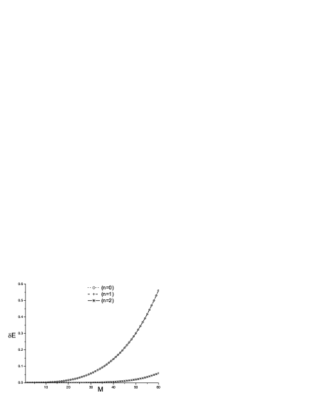
Figure 4: Relative error, $\delta E(M)=\max(\frac{E(M)-E^{(n)}(M)}{\Delta E(M)})$, for three different orders of accuracy ($n=0,1,2$). Here, $E(M)$ is the exact spectrum of the Hamiltonian Eq.(III) calculated numerically in the irrep specified by given M and r values, $\Delta E(M)$ is an average splitting between the spectrum levels, and $E^{(n)}(M)$ is the spectrum calculated by Eq.(40) in n-th order with respect to $\alpha$. For the condensate, we choose ${\cal N}=1000$, hence $r={\cal N}/2$. For the field, the parameters $\Delta/\omega_{p}=2.4\mathrm{E\!-\!8}$, $k_{1}/\omega_{p}=3.04\mathrm{E\!-\!7}$, $k_{2}/\omega_{p}=-3.01\mathrm{E\!-\!9}$ are taken according to the consideration in the previous section.

In Fig. 4 we compare the second order solution Eq.(40) with the exact numerical diagonalization of $H$ Eq.(III) and find that the approximation is very accurate and doesn’t significantly depend on the number $\cal N$ of the particles in the condensate. Basically, as higher the ratio $\frac{|M-2r|}{2r}$ is as better the analytical solution Eq. (40) becomes. The first order correction to the spectrum (of order $\beta_{1}$ in Eq. (40)) is proportional to the detuning $\Delta$ and vanishes at the point of exact resonance. Therefore, the relative error decreases significantly only if the second order correction is taken into account. One can understand from Fig. 4 that at the points where zero and first order errors increase to 50% our second order correction provides accuracy even higher than 95%. The plot depicts typical behavior of the second order solution in the nearby zones. According to the condition Eq. (37) the approximation diverges when we approach too close to the point $|k_{1}/k_{2}|-1=100$. Therefore, we restrict our initial state of the system to the maximum of 60 excitations. It is justified in the next section from physical point of view.

V Subpoissonian distribution in photon statistics

To study photon statistics we have to construct the time evolution of corresponding field operators. It is well-known that the simplest characteristic of subpoissonian nature of the photon distribution is the Fano-Mandel parameter Q(t) defined as follows

$$Q(t)=\frac{\langle(a^{\dagger}a)^{2}\rangle-\langle a^{\dagger}a\rangle^{2}}{\langle a^{\dagger}a\rangle}-1.$$ (41)

Our unitary transformation approach allows to represent the averages of field operators in Eq.(41) in the following convenient form:

$$\langle A(t)\rangle=\langle\Phi_{0}|e^{iHt}Ae^{-iHt}|\Phi_{0}\rangle\approx$$

$$\langle\Phi_{0}|U_{0}^{-1}\left({e^{iH_{diag}^{(2)}t}U_{0}AU_{0}^{-1}e^{-iH_{diag}^{(2)}t}}\right)U_{0}|\Phi_{0}\rangle,$$ (42)

where $|\Phi_{0}\rangle$ is an initial state of the atom-field system and $A$ is an arbitrary operator. In Eq. (V) we left only zero order terms with respect to $\alpha$, i.e. $U_{1,2}\rightarrow 1$, but the diagonalized Hamiltonian $H_{diag}^{(2)}(\tilde{S}_{3})$ is kept up to second-order terms because the time intervals of interest may be relatively large. Applying the relation $a^{\dagger}a=M-\tilde{S}_{3}-\tilde{r}$ it is straight forward to find the time dependence of $A=a^{\dagger}a$ from Eq.(V). The result reads

$$e^{iH_{diag}^{(2)}t}U_{0}\,a^{\dagger}a\,U_{0}^{-1}e^{-iH_{diag}^{(2)}t}=M-\tilde{r}-\frac{\Delta}{\Omega_{R}}\tilde{S}_{3}+$$

$$\frac{k}{2\Omega_{R}}\left({\tilde{S}_{+}e^{it\left[{H_{diag}^{(2)}(\tilde{S}_{3}+1)-H_{diag}^{(2)}(\tilde{S}_{3})}\right]}+h.c.}\right).$$ (43)

Taking the square of the expression Eq.(V) one easily finds corresponding formulae for $A=(a^{\dagger}a)^{2}$. To calculate the parameter Q(t) we have to average these operators over unitary transformed initial state, i.e. over $U_{0}|\Phi_{0}\rangle$. The transformation $U_{0}$ is studied in detail in the theory of the su(2) algebra. If we succeed to represent the initial atom-field state $|\Phi_{0}\rangle$ in the basis of eigenstates $|\tilde{m},\tilde{r}\rangle$ of the operator $\tilde{S}_{3}$ then the corresponding amplitudes $B_{\tilde{m},\tilde{m}1}$ in the expansion $|\tilde{m},\tilde{r}\rangle_{dr}\equiv U_{0}|\tilde{m},\tilde{r}\rangle=\sum_{\tilde{m}1=-\tilde{r}}^{\tilde{r}}B_{\tilde{m},\tilde{m}1}|\tilde{m}1,\tilde{r}\rangle$ can be taken from a textbook. The state $|\tilde{m},\tilde{r}\rangle_{dr}$ is usually called generalized atom-field dressed state.

In the paper we choose a typical initial state of the system, which seems natural for the experiments with sodium BEC. The probe field is prepared in a coherent state with average number of photons $n_{0}=25$. The atoms are prepared in completely symmetrized unexcited eigenstate of the operator $S_{3}$, i.e. $|m_{0},r={\cal N}/2\rangle$, with zero number of excitations ($m_{0}+\frac{\cal N}{2}=0$). Hence,

$$|\Phi_{0}\rangle=|-\frac{\cal N}{2},\frac{\cal N}{2}\rangle\otimes\sum\limits_{n=0}^{\infty}\sqrt{e^{-n_{0}}\frac{n_{0}^{n}}{n!}}\,|n\rangle$$

$$=\sum\limits_{n=0}^{\infty}\sqrt{e^{-n_{0}}\frac{n_{0}^{n}}{n!}}\,|\tilde{m}=-\frac{n}{2},\tilde{r}=\frac{n}{2}\rangle.$$ (44)

The last equality follows from the relations Eqs. (21) and (27), because for completely unexcited atoms the total number of excitations $M$ is equal to the number of photons $n$. Having represented the initial state in the basis of the eigenvectors of the operator $\tilde{S}_{3}$ we can immediumtely calculate the Fano-Mandel parameter $Q$. Below in Fig. 5 we plot the evolution of Q(t) and the average number of photons for such initial state. Regions where the parameter $Q(t)$ takes negative values correspond to subpoissonian distribution in statistics of photons in the probe pulse. First, we notice that the minimum of $Q(t)$ is reached after the second Rabi oscillation, which is described by corresponding Rabi frequency $\Omega_{R}$ given in Eq. (39). The frequency depends on the number of excitations $M$. Being calculated for the average initial number of excitations $M=n_{0}$ it gives the period of Rabi oscillation $T_{R}=2\pi/\Omega_{R}=0.12ns$, which is confirmed by Fig. 5 (see the dynamics of the average number of photons). The time interval where the probe pulse obtains maximum squeezing in fluctuations of the number of photons at, is approximately 0.5ns that is much smaller than the relaxation times in BEC ($T_{rel}=16.3ns$). This time scale satisfies the adiabatic condition imposed at the beginning. The dispersion of photons in the initial coherent state is equal to the average number of photons, i.e. to $n_{0}=25$. It means that the probability to find more than $2n_{0}=50$ photons is negligible and the restriction from above on the number of excitations $M<|k_{1}/k_{2}|\approx 100$ in the system is fulfilled as well.

Figure 5: The Fano-Mandel parameter Q(t) and the average number of photons for initially unexcited sodium BEC and a coherent probe field with $n_{0}=25$ average number of photons. All the parameters are the same as in Fig. 4. The solid line (1) on the plot of $Q(t)$ is calculated in second order of $\alpha$ according to Eq. (V). The dotted line (2) is calculated by Eqs. (45) and (V).

We can notice in Fig. 5 that the maximum squeezing is relatively large, $Q\approx-0.6$. It is observed after two cycles of almost complete absorption and re-emission of the photons by sodium BEC that is represented by the plot of the average number of photons in the probe pulse in Fig. 5. The quantum effect is provided by the correlation in the atomic system, which is transferred to the field after two complete Rabi cycles of the collective atom-field quasi-spin $\tilde{S}_{3}$.

The inline plot of the parameter $Q(t)$ at large time scale shows that the effect has very short life-time and only appears at the beginning. The regular collapses and revivals are observed due to the interference between Rabi oscillations with different frequencies. The effect is well-known in the one-atom case, and the collapse and revival times were estimated in the single-particle modelEberly et al. (1980). We will show now that due to the nonlinear interaction between sodium atoms and the probe pulse the maximum squeezing of photon statistics is achieved much faster than in the regular Dicke model. The fact plays crucial role if one takes into account different mechanisms of the decoherence and relaxation in the system. For instance, the adiabatic approach developed in the paper would break down without the nonlinear terms in the Hamiltonian.

Since we are interested in a short time-scale dynamics, we can neglect higher order corrections to the spectrum of the Hamiltonian Eq. (40) keeping only zero order terms in Eq. (V). Then, we find

$$\langle a^{\dagger}a(t)\rangle=\langle\Phi_{0}|(M-\tilde{r})(1-\cos(\Omega_{R}t))\sin(\psi_{0})^{2}|\Phi_{0}\rangle+\langle\Phi_{0}|a^{\dagger}a\left({\cos(\psi_{0})^{2}+\sin(\psi_{0})^{2}\cos(\Omega_{R}t)}\right)|\Phi_{0}\rangle,$$ (45)

$$\langle a^{\dagger}a(t)^{2}\rangle=\langle\Phi_{0}|(a^{\dagger}a)^{2}\;\left[{\cos(\psi_{0})^{4}+\cos(\psi_{0})^{2}\sin(\psi_{0})^{2}(3\cos(\Omega_{R}t)-1)+\frac{1}{4}\sin(\psi_{0})^{4}(1+3\cos(\Omega_{R}t))}\right]|\Phi_{0}\rangle$$

$$+\langle\Phi_{0}|a^{\dagger}a\;\left[{(M-\tilde{r})\sin(\psi_{0})^{2}\sin(\frac{\Omega_{R}}{2}t)^{2}\left({5+3\cos(2\psi_{0})+6\sin(\psi_{0})^{2}\cos(\Omega_{R}t)}\right)}\right]|\Phi_{0}\rangle$$ (46)

$$+\langle\Phi_{0}|\left[{\frac{1}{2}\sin(\psi_{0})^{2}\sin(\frac{\Omega_{R}}{2}t)^{2}\left({3\tilde{r}(\tilde{r}+1)-(M-\tilde{r})^{2}+(\tilde{r}(\tilde{r}+1)-3(M-\tilde{r})^{2})(\cos(2\psi_{0})+2\cos(\Omega_{R}t)\sin(\psi_{0})^{2})}\right)}\right]|\Phi_{0}\rangle.$$

Notice, that $M,\cos(\psi_{0}),\sin(\psi_{0}),\tilde{r},\Omega_{R}$ are not c-numbers but Casimir operators, so they have to be averaged over the initial state as well as the operator of the number of photons (see the example in Appendix B). The equations Eqs. (45) and (V) are derived in the assumption that the initial state of atoms have zero dipole momentum. But the inversion in the atomic system is allowed to have nonzero values. Our initial state satisfies the condition and the comparison of second order and zero order calculations is provided in Fig. 5 for $Q(t)$. At short time scales the agreement is very good.

In a similar way as it was done by Eberly and co-workers Eberly et al. (1980), we calculate the characteristic times of collapses and revivals in the system by the saddle-point approach. The details are provided in Appendix B. The revival time $\tau_{rev}$ is determined by the difference between two adjacent Rabi frequencies $\Omega_{R}$ with $M=n_{0}$ and $M=n_{0}+1$. The collapse time $\tau_{col}$ has two different asymptotics. In the case of very small $k_{2}$

$$\tau_{col}^{(1)}\approx\sqrt{\frac{4(3r-m_{0}+1)k_{1}^{2}+\Delta^{2}}{k_{1}^{4}\sqrt{n_{0}}}}$$ (47)

and for relatively large nonlinearity but small $1/r$

$$\tau_{col}^{(2)}=\frac{1}{k_{2}\sqrt{\sqrt{n_{0}}r}}.$$ (48)

In Fig. 6 we demonstrate a good agreement between these zero order estimates for different ratios $k_{2}/k_{1}$, and the numerical results. It is worth to notice that according to Eq. (48) the collapse time decreases as $k_{2}^{-1}$ allowing to achieve significant squeezing before the relaxation processes take place. As we showed the nonlinear term provides additional control on the time-scale of quantum effects observed in the system.

Figure 6: The average number of photons for three different combinations of the coupling constants $k_{1},k_{2}$. All parameters are the same as in Fig. 4. The coupling constants and the characteristic time scales are given in Table 1.

Table 1: Characteristic time scales for three different combinations of the coupling constants in sodium BEC.

	$k_{1}/\omega$	$k_{2}/\omega$	$T_{R}$(ns)	$\tau_{col}^{(1)}$ (ns)	$\tau_{col}^{(2)}$ (ns)	$\tau_{rev}$ (ns)
a)	$3\mathrm{E\!-\!7}$	$-3\mathrm{E\!-\!9}$	0.12	41.1.	2.1	19.9
b)	$3\mathrm{E\!-\!7}$	$-3\mathrm{E\!-\!10}$	0.10	41.1	20.8	138
c)	$3\mathrm{E\!-\!6}$	$-3\mathrm{E\!-\!10}$	0.01	4.1	20.8	34

VI Conclusion

In the paper, we studied different mechanisms of the nonlinear interaction between multi-photon optical pulses and many-particles BEC. The dynamics corresponds to a regime of giant delays in the probe pulse propagation with almost negligible absorption of the pulse in the medium with electro-magnetically induced transparency. Taking the advantage of using tree-level $\Lambda$-scheme within polarization approach we find an explicit form of the linear and nonlinear susceptibilities of the atomic condensate characterized with significant transparency induced by the classical field. We studied properties of the condensate refraction index and absorption coefficient related to the probe pulse at frequencies close to the frequency of corresponding atomic transition. It was demonstrated that the nonlinear refraction index can reach extremely large values. The regions of its negative values and nonlinear dependence of the absorption on the pulse intensity provide a possibility to achieve almost complete compensation of the losses and the dispersion in the BEC.

Applying the formalism of polynomially deformed su(2) algebras we analyze complex quantum dynamics of the probe pulse in a coherent ensemble of sodium atoms. It was shown that the nonlinear effects provide a necessary window in the relaxation mechanisms where the probe pulse in the regime of ”slow” light exhibits nonclassical properties in statistics of photons. We demonstrated that the poissonian statistics of photons in the coherent state of the probe pulse can be significantly squeezed within short period of time to highly subpoissonian values due to collective interaction between coherent atoms and the field. These results open new perspectives in generation of nonclassical atomic or field states in Bose-Einstein condensate controlled by external classical light.

Appendix A Unitary transformations

After the transformation $U_{0}=e^{i\psi_{0}\tilde{S}_{y}}$ the Hamiltonian Eq. (38) reads

$$U_{0}H^{(2)}U_{0}^{-1}=C_{0}+\Omega_{R}\tilde{S}_{3}-k\frac{\beta_{1}}{4}\left[{\cos(2\psi_{0})\left({\tilde{S}_{3}\tilde{S}_{x}+\tilde{S}_{x}\tilde{S}_{3}}\right)+\sin(2\psi_{0})\left({\tilde{S}_{3}^{2}-\tilde{S}_{x}^{2}}\right)}\right]$$

$$-k\frac{\beta_{2}}{2}\left[{\begin{array}[]{c}(\cos(3\psi_{0})+\cos(\psi_{0})\sin(\psi_{0})^{2})\tilde{S}_{3}\tilde{S}_{x}\tilde{S}_{3}-(\sin(3\psi_{0})-\sin(\psi_{0})\cos(\psi_{0})^{2})\tilde{S}_{x}\tilde{S}_{3}\tilde{S}_{x}\\ +\sin(\psi_{0})\tilde{S}_{3}\left({\cos(\psi_{0})^{2}(\tilde{S}_{3}^{2}-1)+\frac{1}{4}}\right)+\cos(\psi_{0})\tilde{S}_{x}\left({\sin(\psi_{0})^{2}(\tilde{S}_{x}^{2}-1)+\frac{1}{4}}\right)\\ \end{array}}\right].$$ (51)

To diagonalize the operator Eq. (A) in first order of $\beta_{1}\sim\alpha$ we apply second unitary transformation

$$U_{1}=\exp{\left[{-i\frac{\beta_{1}}{4}\sin(\psi_{0})\left({(\tilde{S}_{3}\tilde{S}_{y}+\tilde{S}_{y}\tilde{S}_{3})\cos(2\psi_{0})-\frac{1}{4}(\tilde{S}_{x}\tilde{S}_{y}+\tilde{S}_{y}\tilde{S}_{x})\sin(2\psi_{0})}\right)}\right]}.$$ (52)

It is obvious that the transformation $U_{1}$ applied to the zero order term in Eq. (A) gives the first order term in the original Hamiltonian but with an opposite sign providing that it is cancelled. Thus, the Hamiltonian $U_{1}U_{0}H^{(2)}U_{0}^{-1}U_{1}^{-1}$ is diagonal up to second order of $\alpha$. It has the form

$$U_{1}U_{0}H^{(2)}U_{0}^{-1}U_{1}^{-1}=C_{0}+\Omega_{R}\tilde{S}_{3}-k\frac{\beta_{1}}{4}\sin(\psi_{0})\cos(\psi_{0})\left({3\tilde{S}_{3}^{2}-\tilde{r}(\tilde{r}+1)}\right)$$

$$+k\left({\frac{\beta_{1}}{4}}\right)^{2}\sin(\psi_{0})\left[{\begin{array}[]{c}\cos(2\psi_{0})^{2}\tilde{S}_{3}(4\tilde{S}_{3}^{2}-2\tilde{r}(\tilde{r}+1)+\frac{1}{2})+\frac{\sin(2\psi_{0})^{2}}{4}\tilde{S}_{3}(5\tilde{S}_{3}^{2}-5\tilde{r}(\tilde{r}+1)+\frac{11}{2})\\ +3\sin(2\psi_{0})^{2}\tilde{S}_{x}\tilde{S}_{3}\tilde{S}_{x}-\frac{\sin(4\psi_{0})}{2}\left({9\tilde{S}_{3}\tilde{S}_{x}\tilde{S}_{3}+\tilde{S}_{x}^{3}-\frac{6\tilde{r}(\tilde{r}+1)-13}{4}\tilde{S}_{x}}\right)\\ \end{array}}\right]$$ (55)

$$-k\frac{\beta_{2}}{2}\left[{\begin{array}[]{c}(\cos(3\psi_{0})+\cos(\psi_{0})\sin(\psi_{0})^{2})\tilde{S}_{3}\tilde{S}_{x}\tilde{S}_{3}-(\sin(3\psi_{0})-\sin(\psi_{0})\cos(\psi_{0})^{2})\tilde{S}_{x}\tilde{S}_{3}\tilde{S}_{x}\\ +\sin(\psi_{0})\tilde{S}_{3}\left({\cos(\psi_{0})^{2}(\tilde{S}_{3}^{2}-1)+\frac{1}{4}}\right)+\cos(\psi_{0})\tilde{S}_{x}\left({\sin(\psi_{0})^{2}(\tilde{S}_{x}^{2}-1)+\frac{1}{4}}\right)\\ \end{array}}\right].$$ (58)

Notice that we only keep terms of order $\alpha$ or $\alpha^{2}$. Therefore, the last term in Eq. (A) stays intact after the transformation. One can see that the first order correction vanishes in the case of exact resonance $\Delta=0$. So, it is necessary to consider second order terms to take into account significant effects connected with the nonlinear dependence of the energy splitting on the value of collective atom-field quasi-spin vector $\tilde{S}_{3}$.

To diagonalize the operator Eq. (A) up to the order $\alpha^{2}$ we apply the third unitary transformation

$$U_{2}=\exp{\left[{\begin{array}[]{c}i\left({\frac{\beta_{1}}{4}\sin(\psi_{0})}\right)^{2}\left\{{\frac{3}{4}\sin(\psi_{0})^{2}(\tilde{S}_{x}\tilde{S}_{3}\tilde{S}_{y}+\tilde{S}_{y}\tilde{S}_{3}\tilde{S}_{x})+\frac{\sin(4\psi_{0})}{2}\left({\frac{1}{3}\tilde{S}_{y}^{3}-8\tilde{S}_{3}\tilde{S}_{y}\tilde{S}_{3}+\frac{\tilde{r}(\tilde{r}+1)}{2}\tilde{S}_{y}-\frac{31}{12}\tilde{S}_{y}}\right)}\right\}\\ -i\frac{\beta_{2}}{2}\sin(\psi_{0})\left\{{\begin{array}[]{c}2\cos(3\psi_{0})\tilde{S}_{3}\tilde{S}_{y}\tilde{S}_{3}+\frac{1}{2}\cos(\psi_{0})\tilde{S}_{y}+\frac{1}{2}\sin(\psi_{0})\cos(\psi_{0})^{2}(\tilde{S}_{y}\tilde{S}_{3}\tilde{S}_{x}+\tilde{S}_{x}\tilde{S}_{3}\tilde{S}_{y})\\ -\frac{\sin(3\psi_{0})}{2}(\tilde{S}_{y}\tilde{S}_{3}\tilde{S}_{x}+\tilde{S}_{x}\tilde{S}_{3}\tilde{S}_{y})-\cos(\psi_{0})\sin(\psi_{0})^{2}\tilde{S}_{y}(\frac{2}{3}\tilde{S}_{y}^{2}-2\tilde{r}(\tilde{r}+1)+\frac{10}{3})\\ \end{array}}\right\}\\ \end{array}}\right]}.\quad$$ (63)

Consecutively applying these three transformations $U_{0,1,2}$ to the Hamiltonian Eq. (38) we obtain the diagonal operator Eq. (40).

Appendix B The collapse and revival characteristic times

According to the zero-order solution Eq.(45) a dynamics of the average number of photons for the initial state Eq.(V) has the form

$$\bar{n}(t)=\sum\limits_{n=0}^{\infty}\frac{nn_{0}^{n}e^{-n_{0}}}{n!}\frac{k_{n}^{2}+2\Delta^{2}+k_{n}^{2}\cos(\sqrt{k_{n}^{2}+\Delta^{2}}t)}{2(k_{n}^{2}+\Delta^{2})},\quad$$ (64)

where based on Eqs. (35) and (36) we defined

$$k_{n}=\left({k_{1}+k_{2}\frac{n+1}{2}}\right)\sqrt{2(4r-n+1)}.$$ (65)

Deriving the expressions we used the fact that our initial state belongs to the nearby zones ($\tilde{r}=M/2$) and the atoms are completely unexcited ($M=n,m_{0}=-r$). For simplicity of the analytical expressions below, we represent the results taking $m_{0}=-r$. But they can easily be generalized for arbitrary initial number of excitations in atomic subsystem. Since we are interested in the time dependence of $\bar{n}(t)$, the constant terms in Eq. (64) can be discarded. We estimate the sum of the time depending term using the saddle-point method, which has been applied to calculate the one-atom model Eberly et al. (1980). Denoting the time dependent term in Eq. (64) by $w(t)$ we can write

$$w(t)\approx\int\limits_{0}^{\infty}\sqrt{\frac{n}{2\pi}}\frac{k_{n}^{2}}{2(k_{n}^{2}+\Delta^{2})}Re\left({e^{-n_{0}+n_{0}f(n/n_{0})}}\right)\,dn,\quad$$ (66)

where

$$f(x)=x(1-\ln x)$$

$$+it\sqrt{\frac{\Delta^{2}}{n_{0}^{2}}+\left({2r+\frac{1}{2}-\frac{n_{0}x}{2}}\right)\left({\frac{2k_{1}+k_{2}}{n_{0}}+k_{2}x}\right)^{2}}.$$ (67)

Using the approach we find

$$w(t)\approx\frac{n_{0}k_{n_{0}}^{2}}{2(k_{n_{0}}^{2}+\Delta^{2})}Re\left({\frac{e^{-n_{0}+n_{0}f(x_{0})}}{\sqrt{f^{\prime\prime}(x_{0})}}}\right),$$ (68)

where the point $x_{0}$ is the saddle-point of the analytical function $f(x)$, i.e. $f^{\prime}(x_{0})=0$. It follows from the definition that the saddle-point $x_{0}$ depends on the time. As it was explained in detail in the paper Eberly et al. (1980), the collapse time $\tau_{col}$ is roughly estimated by the condition

$$\left|{1-Ref(x_{0})}\right|=\sqrt{n_{0}}.$$ (69)

For the moment $\tau_{col}$ when the condition Eq. (69) is fulfilled, the exponent in Eq. (68) becomes very small and the envelope of the sinusoidal oscillations ”collapses”. For $t=0$ it is plain to see that $x_{0}=1$.

Expanding the solution for $x_{0}$ in the vicinity of unity and substituting it into Eq. (69) we obtain relatively lengthy expression. If we assume that the nonlinear susceptibility $k_{2}$ is the dominating smallness parameter, and expand the result with respect to $k_{2}\rightarrow 0$, we find

$$\tau_{col}^{(1)}\approx\sqrt{\frac{4(3r-m_{0}+1)k_{1}^{2}+\Delta^{2}}{k_{1}^{4}\sqrt{n_{0}}}+4k_{2}\frac{k_{1}^{2}(8r-n_{0}+1)(4r+1)-(2r-n_{0})\Delta^{2}}{k_{1}^{5}\sqrt{n_{0}}}}.$$ (70)

Assuming that the leading smallness parameter is $1/r$ we obtain an expression for relatively large nonlinearity $k_{2}$

$$\tau_{col}^{(2)}=\frac{1}{k_{2}\sqrt{\sqrt{n_{0}}r}}\sqrt{1+\frac{8k_{1}^{4}+6k_{1}^{2}k_{2}^{2}(2n_{0}+1)+4k_{1}^{3}k_{2}(2n_{0}+3)+k_{1}k_{2}^{3}(\frac{\Delta^{2}}{k_{2}^{2}}+6n_{0}+1)+k_{2}^{4}(n_{0}-\frac{\Delta^{2}}{k_{2}^{2}}(n_{0}-\frac{1}{2}))}{2rk_{2}(2k_{1}+k_{2})^{3}}}.\quad$$ (71)

Even for $k_{2}=0$ in the Eq. (70) our results can’t be straightforward compared with Eberly’s paper because we consider the dynamics in the nearby zones, which do not exist in the simple one-atom model. But, it is not a problem to obtain corresponding results for the remote zones, which are more relevant to their work. We also want to notice that the solutions Eq. (70) and (71) provide additional information about the dependence of collapse times on the number of particles in BEC, which is completely opposite in these two asymptotics.

The revival time is estimated by the period when the phases of oscillations of neighboring terms in Eq. (64) with frequencies $k_{n}$ differ by $2\pi$. The difference is estimated for the dominant sinusoids with $n=n_{0}$ and $n=n_{0}+1$. The revival time reads

$$\tau_{rev}\approx\left|{\frac{2\pi}{\sqrt{k_{n_{0}+1}^{2}+\Delta^{2}}-\sqrt{k_{n_{0}}^{2}+\Delta^{2}}}}\right|.$$ (72)

The Rabi oscillation period $T_{R}$ in Table 1 is estimated as

$$T_{R}\approx\frac{2\pi}{\sqrt{k_{n_{0}}^{2}+\Delta^{2}}}.$$ (73)

References

- Scully and Zubairy (1997) M. Scully and M. Zubairy, Quantum Optics (Cambridge University Press, Cambridge, England, 1997).
- Wolf (2002) E. Wolf, in Progress In Optics, ed. by Elsevier Science B. V., Netherlands, Amsterdam 43, 512 (2002).
- Imamoglu et al. (1997) A. Imamoglu, H. Schmidt, G. Woods, and M. Deutsch, Phys. Rev. Lett. 79, 1467 (1997).
- Wang et al. (2002) H. Wang, D. Goorskey, and M. Xiao, Opt. Lett. 27, 258 (2002).
- Basov et al. (1966) N. Basov, R. Abartsumian, V. Zuev, and et. al., JETP 23, 16 (1966).
- Basov and Letokhov (1966) N. Basov and V. Letokhov, Sov. Dokl. 11, 222 (1966).
- Garrett and McCumber (1970) C. G. B. Garrett and D. E. McCumber, Phys. Rev. A 1, 305 (1970).
- Chu and Wong (1982) S. Chu and S. Wong, Phys. Rev. Lett. 48, 738 (1982).
- Allen and Ebebley (1978) L. Allen and J. Ebebley, Optical resonans and two-level atoms (Mir, Moscow, 1978).
- Harris et al. (1990) S. E. Harris, J. E. Field, and A. Imamoglu, Phys. Rev. Lett. 64, 1107 (1990).
- Alzetta et al. (1976) G. Alzetta, A. Gozzini, L. Moi, and G. Orriols, Nuovo Cimento 36B, 5 (1976).
- Gray et al. (1978) H. R. Gray, R. M. Whitley, and C. R. Stroud, Opt. Lett. 3, 218 (1978).
- Tewari and Agarwal (1986) S. P. Tewari and G. S. Agarwal, Phys. Rev. Lett. 56, 1811 (1986).
- Harris et al. (1992) S. E. Harris, J. E. Field, and A. Kasapi, Phys. Rev. A 46, R29 (1992).
- Turukhin et al. (2002) A. V. Turukhin, V. S. Sudarshanam, M. S. Shahriar, and et al., Phys. Rev. Lett. 88, 023602 (2002).
- Lukin et al. (1998) M. D. Lukin, P. Hemmer, M. Loffler, and M. O. Scully, Phys. Rev. Lett. 81, 2675 (1998).
- Wang et al. (2001) H. Wang, D. Goorskey, and M. Xiao, Phys. Rev. Lett. 87, 073601 (2001).
- Ketterle (2002) W. Ketterle, Rev. Mod. Phys. 74, 1131 (2002).
- Cornell and Wieman (2002) E. A. Cornell and C. E. Wieman, Rev. Mod. Phys. 74, 875 (2002).
- Hau et al. (1999) L. N. Hau, S. E. Harris, Z. Dutton, and C. H. Behroozi, Lett. to Nature 397, 594 (1999).
- McClelland and Kelley (1985) J. McClelland and M. Kelley, Phys. Rev. A 31, 3704 (1985).
- Mitsunaga et al. (2000) M. Mitsunaga, M. Yamashita, and H. Inoue, Phys. Rev. A 62, 013817 (2000).
- Leontovich (1944) M. Leontovich, Sov. Izv., Ser. Phys. 8, 16 (1944).
- Patnaik et al. (2002) A. K. Patnaik, J. Q. Liang, and K. Hakuta, Phys. Rev. A 66, 063808 (2002).
- R.Shen (1984) Y. R.Shen, The Principles of Nonlinear Optics, ed. by John Wiley and Sons (University of California, Berkeley, 1984).
- Lukin and Imamog?lu (2000) M. D. Lukin and A. Imamog?lu, Phys. Rev. Lett. 84, 1419 (2000).
- Agrawal (2001) G. P. Agrawal, Nonlinear Fiber Optics, ed. by Academic Press (USA, San Diego, 2001).
- Al-Awfi and Babiker (2000) S. Al-Awfi and M. Babiker, Phys. Rev. A 58, 4768 (2000).
- Mitchell and Chiao (1997) M. Mitchell and R. Chiao, Phys. lett. A 230, 133 (1997).
- Tavis and Cummings (1968) M. Tavis and F. Cummings, Phys. Rev. 170, 379 (1968).
- Dicke (1954) R. Dicke, Phys. Rev. 93, 99 (1954).
- Andre and Lukin (1954) A. Andre and M. D. Lukin, Phys. Rev. Lett. 89, 143602 (1954).
- Icsevgi and Lamb (1954) A. Icsevgi and W. E. Lamb, Phys. Rev. 185, 517 (1954).
- Vadeiko et al. (2003) I. Vadeiko, G. Miroshnichenko, A. Rybin, and J. Timonen, Phys. Rev. A 67, 053808 (2003).
- Chumakov et al. (1994) S. Chumakov, A. Klimov, and J. Sanchez-Mondragon, Phys. Rev. A 49, 4972 (1994).
- Saavedra et al. (1998) C. Saavedra, A. Klimov, S. Chumakov, and J. Retamal, Phys. Rev. A 58, 4078 (1998).
- Delgado et al. (2001) J. Delgado, E. Yustas, L. Sanchez-Soto, and A. Klimov, Phys. Rev. A 63, 063801 (2001).
- Eberly et al. (1980) J. Eberly, N. Narozhny, and J. Sanchez-Mondragon, Phys. Rev. Lett. 44, 1323 (1980).