and ]College of Judea and Samaria, Ariel 44284, Israel

Phase Evolution in a Multi-Component System

Abstract

We derive a general expression for the expectation value of the phase acquired by a time dependent wave function in a multi component system, as excursions are made in its coordinate space. We then obtain the mean phase for the (linear dynamic $E\otimes\epsilon$) Jahn-Teller situation in an electronically degenerate system. We interpret the phase-change as an observable measure of the effective nodal structure of the wave function.

In a recent publication a geometric (or Berry) phase was calculated for the wave function of a multi-component closed system FuentesGCBV . This differs from the usually considered situations, in which the Berry phases emerge from the wave-function of the system during the cyclic evolution of some external parameter. It is of interest to point out that in a famous prototype of a multi-component, closed system (an electronically doubly degenerate molecule) dynamic solutions for the $E\otimes\epsilon$ linear Jahn-Teller effect (DJTE) were fully obtained as long ago as 1957 MoffitT ; LonguetOPS . The two parts of system were the electronic and ionic constituents of the molecule. Though this has received, as just noted, a complete treatment early on, the dynamic problem has not left the scientific agenda ever since. Descriptions of some of the early refinements are found in two books Englman ; BersukerP ; the most recent publication known to us and involving a variational treatment of the problem is in DunnE . The physical consequences of the Berry phase on the DJTE were clearly brought out by the late Frank Ham Ham and more recently in KoizumiB , both of which papers showed (albeit under different physical conditions) that the value of the Berry phase may be critical in determining the order of energy levels in the closed molecular system. This phase is thus clearly observable by experiment Ham . Its physical interpretation, essentially along the lines of Ham ; KoizumiB , will be given later in this work.

In FuentesGCBV an operator was proposed for the phase change (called ”quantized phase”) in a closed system. Here we shall derive an expression for this phase from first principles and use it to calculate the phase change in the vibronic doublet ground states of an $E\otimes\epsilon$ linearly coupled Jahn-Teller system. We shall use a ”guessed solution”, for the ground state, which is transparent, intuitively simple and algebraically easily manageable Englman62 ; EnglmanH ; Englman . Though not variationally obtained, the ”guessed solution” was found to have eigen-energies that are considerably closer to the exact, computed energies of LonguetOPS than any other approximate solution with which it was compared. This comparison is seen in Fig. 2 of ZhengB . Later treatments did not test their methods by comparison with the ”guessed solution”.

Our point of departure is the time-dependent Schrödinger equation

$$i\frac{\partial}{\partial t}\psi({\bf r},t)=H({\bf r},t)\psi({\bf r},t)$$ (1)

for a wave function $\psi({\bf r},t)$ that depends on the internal coordinates ${\bf r}$ of the system, as well as on time $t$. ($\hbar=1$) The system is coupled to the environment; hence the dependence on $t$ in the Hamiltonian. In a closed system, the Hamiltonian is time-independent. $\psi$ is still time-dependent, as, e.g., in a wave-packet.

We write the state (assumed to be regular in the coordinate space and vanishing at its boundaries) as

$$\psi=Ae^{iS}$$ (2)

with $A$ and $S$ being real functions of ${\bf r},t$. ($A>0$.) We shall utilize the equation of continuity and the Hamilton-Jacobi equation Messiah :

$$\frac{\partial A^{2}}{\partial t}=-\frac{1}{m}\nabla(A^{2}\nabla S)$$ (3)

$$\frac{1}{2m}(\nabla S)^{2}=-\frac{\partial S}{\partial t}-V({\bf r},t)+\frac{1}{2m}A^{-1}(\nabla)^{2}A$$ (4)

Here $m$ is a mass parameter common to all degrees of freedom, with all coordinates scaled to this mass. $V$ is the potential.

Let us now consider the change in the wave function, between the initial state of the system at $t=0$ and a final time $t_{f}$. Real and imaginary parts of the change in the logarithm are

$$[ln\psi]^{t_{f}}_{0}=[ln|\psi|]^{t_{f}}_{0}+i[arg(\psi)]^{t_{f}}_{0}=[lnA]^{t_{f}}_{0}+i[S]^{t_{f}}_{0}$$ (5)

These are functions of the coordinates. To form quantum mechanical expectation values (denoted by angular brackets about the relevant quantities) we multiply by $A^{2}$ and integrate over all coordinates. Thus the mean of the changes can be written as

$$<[lnA]^{t_{f}}_{0}>+i<[S]^{t_{f}}_{0}>=\int_{0}^{t_{f}}dt\frac{\partial}{\partial t}\int d{\bf r}A^{2}(lnA+iS)$$ (6)

[ It is natural to conjecture that to form statistical expectation values (appropriate to mixed states SjoqvistPEAEOV ), the factor $A^{2}$ is to be multiplied by the relative statistical weight of the state and the contribution due to all states be summed over. We do not pursue this topic here.] Separating real and imaginary parts we get for the real part the quantity $-\frac{1}{2}[{{\cal S}_{e}}]^{t_{f}}_{0}$ where

$${{\cal S}_{e}}=-\int d{\bf r}|\psi|^{2}ln|\psi|^{2}$$ (7)

${\cal S}_{e}$ (which is different from the phase $S$) is reminiscent of a von Neumann entropy, in which the density operator is projected onto the initial state.

We turn now to the rate of change of the expectation value of the phase $\frac{d<S>}{dt}$. We change the order of integrations in equation (6) and obtain after some manipulations :

$$\frac{d<S>}{dt} = \int d{\bf r}(A^{2}\frac{\partial S}{\partial t}~{}+~{}S\frac{\partial A^{2}}{\partial t})=\int d{\bf r}[A^{2}\frac{\partial S}{\partial t}~{}-~{}\frac{1}{m}S\nabla(A^{2}\nabla S)]$$ (8)

$$= \int d{\bf r}[A^{2}\frac{\partial S}{\partial t}+\frac{1}{m}A^{2}(\nabla S)^{2}]$$

having used equation (3) and integrated by parts (with vanishing integrands at space-extremities). We now substitute for $(\nabla S)^{2}$ from equation (4) and obtain a change in the sign of the first term in the above expression, as well as the expectation values of (twice) the potential and a term related to the kinetic energies, which can be reworked by a further integration by parts so as to put it into a form of definite sign, giving

$$\frac{d<S>}{dt}=-\int d{\bf r}(A^{2}\frac{\partial S}{\partial t})~{}-~{}2<V({\bf r},t)>~{}-~{}\frac{1}{m}\int d{\bf r}(\nabla A)^{2}$$ (9)

We next recall that $S=Im(ln\psi)$ and reinstate the time integration to get the change of phase as

$$[<S>]^{t_{f}}_{0} = -\int^{t_{f}}_{0}dt\int d{\bf r}[Im(\psi^{+}({\bf r},t)\frac{\partial\psi({\bf r},t)}{\partial t})+2|(\psi({\bf r},t)|^{2}V({\bf r},t)$$ (10)

$$+ \frac{1}{m}(\nabla|\psi({\bf r},t)|)^{2}]$$

where the cross means Hermitian conjugate. On the other hand, multiplying equation (1) by $\psi^{+}({\bf r},t)$, integrating over the coordinates and again integrating by parts, we obtain

$$Im\int d{\bf r}(\psi^{+}({\bf r},t)\frac{\partial\psi({\bf r},t)}{\partial t})=-\int d{\bf r}\frac{|\nabla\psi({\bf r},t)|^{2}}{2m}-\int d{\bf r}|(\psi({\bf r},t)|^{2}V({\bf r},t)$$ (11)

which we use to eliminate the expectation value of the potential from equation (10) . We then get:

$$[<S>]^{t_{f}}_{0} = Im\int^{t_{f}}_{0}dt\int d{\bf r}(\psi^{+}({\bf r},t)\frac{\partial\psi({\bf r},t)}{\partial t})$$ (12)

$$+ \frac{1}{m}\int^{t_{f}}_{0}dt\int d{\bf r}[|\nabla\psi({\bf r},t)|^{2}-(\nabla|\psi({\bf r},t)|)^{2}]$$

This is our central result for the mean phase change. The first term is of the form familiar in e.g., expressions of the open path geometric phase PatiJ . In the second term, to be denoted for brevity $\delta K$, one has the difference between two space-derivative terms, one involving the total (complex) time-dependent wave-function and the other its modulus.

We now calculate the phase change in our molecular model for a multi-component closed system. The main simplification in the model is the restriction to a two-dimensional electronic subspace (it being assumed that other electronic states of the molecule are too far away to have any effect) and small displacements of the nuclear coordinates from some standard configuration (so that only linear terms in the nuclear displacement coordinates appear in the Hamiltonian below). The solution to the mathematical problem (the DJTE) embodies the correlated nuclear-electronic trajectory near a conical intersection of the (diabatic) potential surfaces. Under these circumstances the usual Born-Oppenheimer approximation breaks down and the description of the combined dynamics is non-trivial.

The total Hamiltonian consists of $H_{mol}$ for the internal degrees of freedom of the molecule and an interaction term with the environment $H_{env}$.

$$H=H_{mol}+H_{env}$$ (13)

The first term is a function of the electronic and nuclear coordinates, while the second term may contain also an externally imposed time dependence. Our restriction to a two-dimensional electronic subspace $|1>,|2>$ removes from the formalism the presence of electronic coordinates and leaves only the nuclear coordinates. Two of these, designated $q_{a},q_{b}$, are of interest. $H_{mol}$ when expressed in terms of the bosonic creation $(a^{+},b^{+})$ and annihilation $(a,b)$ operators of the nuclear motion, takes the form

$$H_{mol}=\frac{\omega}{2}\{a^{+}a+~{}b^{+}b-\frac{k}{\sqrt{2}}[(a^{+}+a)\sigma_{z}-(b^{+}+b)\sigma_{x}]\}$$ (14)

Here $\omega$ is the frequency of oscillation of the nuclear motion, and $k$ is the electron-nuclear coupling strength expressed in dimensionless units. The $2$ x $2$ matrices $\sigma_{x}$ and $\sigma_{z}$ are the familiar Pauli operators acting on the electronic $|1>,|1>$ subspace. Equivalent representations of the Hamiltonian $H_{mol}$ are given in works on the Jahn-Teller effect (Englman62 ; Englman ; BersukerP ); i.e., in terms of the nuclear coordinates $q_{a},q_{b}$ or of the associated cylindrical coordinates $(q,\phi)$, where $q_{a}=qcos\phi,~{}q_{b}=qsin\phi$, as, e.g., in Eq. 3.5 of Englman .

The algebraic expression for the ground state doublet proposed in Englman62 ; EnglmanH , and which solves the time-independent Schrödinger equation for the Hamiltonian $H_{mol}$ to a good approximation, has the following (unnormalized) form:

$$\hat{\psi}(q_{a},q_{b})=\exp-\frac{1}{2}\big{[}(q_{a}-k\sigma_{z})^{2}+(q_{b}+k\sigma_{x})^{2}]$$ (15)

(Intuitively, this form is suggested by analogy with the ground state solutions of displaced harmonic oscillators, but its justification is in its close agreement with exactly computed eigenvalues of $H_{mol}$ LonguetOPS ). To obtain the ground state doublet we operate with $\hat{\psi}(q_{a},q_{b})$ on any two linearly independent combinations of the basic vectors $|1>,|2>$. In a column vector representation these are just ${\tiny\left(\begin{array}[]{cc}1\\ 0\end{array}\right),~{}\left(\begin{array}[]{cc}0\\ 1\end{array}\right)}$. The exponential, which includes non-commuting matrices, can be manipulated by use of the commutation relations between the Pauli-matrices to give, in terms of the cylindrical coordinates defined above, the expression

$$\hat{\psi}(q,\phi)=\exp[-k^{2}-q^{2}/2][\cosh(kq){\bf I}-\sinh(kq)(\sigma_{z}\cos\phi-\sigma_{x}\sin\phi)]$$ (16)

${\bf I}$ is the unit $2$ x $2$ matrix. One notes that this is a single valued function of $\phi$ (there are no $\cos\phi/2$ terms), as indeed is required of the wave function of a closed system Ham .

By operating with $\hat{\psi}$ on ${\frac{1}{\sqrt{2}}}\left(\begin{array}[]{cc}1\\ {\mp}i\end{array}\right)$ one gets the two degenerate ground- state functions $\Psi(q,\phi)(=\Psi_{-})$ and $\Psi^{*}(q,\phi)(=\Psi_{+})$. The eigenvalues and other related properties of these states have been calculated in EnglmanH ; Englman . Here we compute the phase-change for each function, as the angular coordinate changes by a full period between $\phi=0$ and $\phi=2\pi$.

One procedure to induce such change in an internal coordinate (and physically, perhaps, the only consistent one) is to consider it being guided by an external force along a circle. (The concept of a guiding potential was used in, e.g, AharonovB , but here we guide the angular coordinate, rather than the radial one.) To achieve this, one needs an external, time dependent agent acting on the otherwise closed system and this is the role played by $H_{env}$ in the Hamiltonian shown in equation (13) . We suppose that there is an environment Hamiltonian which induces a $delta$-function like behavior in the wave function (forcing $\phi$ to equal $\Omega t$) and that this time-dependent $H_{env}$ dominates the kinetic energy of the angular variable. In this, delta-function limit the variable $\phi$ turns into a (classical) parameter and is no longer a ”degree of freedom”.

We thus get from equation (12) for the expectation value of the phase change in the $\Psi^{-}$ state the expression

$$<[S]^{t_{f}}_{0}> = [Im\int^{t_{f}}_{0}dt[\int^{\infty}_{0}dqq\Psi^{+}_{-}(q,\Omega t)\frac{\partial}{\partial t}\Psi_{-}(q,\Omega t)$$ (17)

$$+ \delta K]/\int^{\infty}_{0}dqq|\Psi_{-}(q,\Omega t)|^{2}]$$

where $\delta K$ is the second term on the right hand side of equation (12) involving the space differentials. In all integrals the integration is over the radial coordinate $q$ only, since $\phi=\Omega t$ is treated as a parameter.

It can be shown that $\delta K$ is identically zero for the both $\Psi_{-}$ and $\Psi_{+}$. (Remember that the gradient operator in $\delta K$ involves now only the radial degree of freedom $q$.) The evaluation of the first integral in equation (17) leads to the plot shown in the following figure for the mean phase after a full cyclic revolution $<[S]^{2\pi/\Omega}_{0}>$ as function of the coupling strength $k$. (Fig. 1)

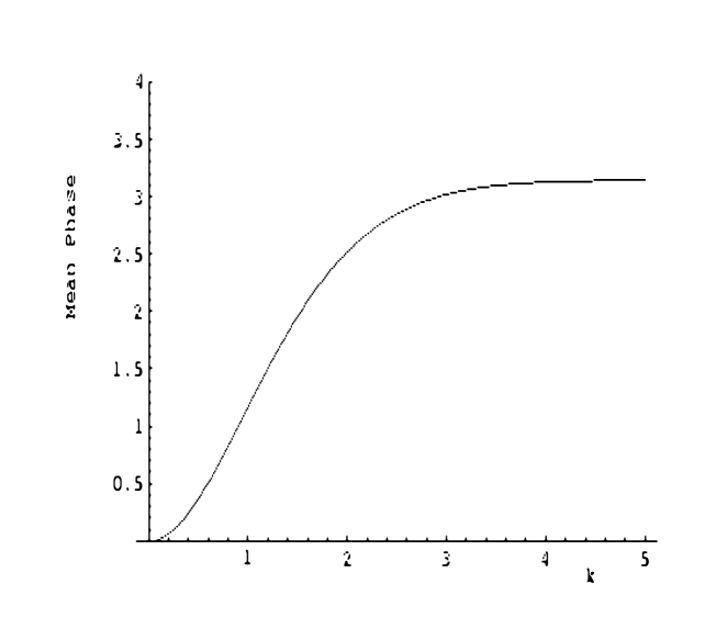
Figure 1: Expectation value of the phase change after a full cycle in the coordinate space versus the coupling strength. We plot $[<S>]^{2\pi/\Omega}_{0}$ ( equation (17) , with $\delta K=0$ ) against k (introduced in equation (13) ). For large $k$, the phase approaches $\pi$.

As seen in the figure, the acquired mean phase for $\Psi_{-}$ increases monotonically with the coupling and levels off for strong coupling $(k>>1)$ to $\pi$ (the value of the Berry-phase). The corresponding phase for the partner state $\Psi_{+}$ is the negative of this value, and any linear combination of the ground state doublet will result in intermediate values between the two extremes $\pm\pi$. The phase depends only on the strength of the coupling $k$. It is independent of the adiabatic parameter $\frac{k\omega}{\Omega}$, since the integrand contains only the instantaneous value of the initial component $\Psi_{-}$ , and no admixture from its partner $\Psi_{+}$ . (Applying our equation (17) to the eigenstates $\Phi_{n}^{\pm}$ of FuentesGCBV expressed in a coordinate representation reproduces exactly the results obtained in that paper. However, evaluation of the expectation value of the phase-shift operator proposed in FuentesGCBV for the states $\Psi^{\pm}(q,\phi)$ in this work, where the rotating-wave approximation is not made, yields values that diverge quadratically for large k.)

We conclude with an interpretation of the ”closed-system” phase. In this we follow Ham ; KoizumiB . For low values of the coupling constant, the wave function is smeared over the origin $q=0$ and cannot be said to circle around this point, which is a point of degeneracy of the two states. Then there is hardly any acquired phase. For large values of the coupling, the wave function is located near $q=k$, meaning that it keeps away from origin, so that circling ${\it around}$ it can achieve the full measure of the geometric phase.

On the other hand, it has been known for some time that (in the adiabatic limit) the phase change comes about abruptly, precisely at the moment of circling when a component amplitude vanishes. (This occurs when $cos\frac{\Omega t}{2}=0$, or $\Omega t=\pi$. The abrupt change is clearly seen in the figures of EnglmanY1999 ; EnglmanYB2000 and has recently formed the subject of a Letter Sjoqvist .) By the interpretation just given, the phase change is a measure of the extent that a circling in the coordinate space scans the zeros of the wave function in the region encircled. Since zeros (nodes) in the wave function are known to affect (in general, raise) the energies of the states, it is natural to find that the phase acquired during a revolution determines the ordering of the energy levels. Such connections between phase change and energy levels have been noted first in Ham and more recently in KoizumiB .

- (1) 9
- (2) I. Fuentes-Guridi, A. Carollo, S. Bose and V. Vedral, Phys. Rev. Lett. 89 220404 (2002)
- (3) W. Moffitt and W. Thorson, Phys. Rev. 106 1251 (1957)
- (4) H.C. Longuet-Higgins, U. Öpik, M.H.L. Pryce and R.A. Sack, Proc. Roy. Soc. London A 244 1 (1958)
- (5) R. Englman, The Jahn-Teller Effect in Molecules and Crystals (Wiley, Chichester, 1972)
- (6) I.B. Bersuker and V.Z. Polinger, Vibronic Interactions in Molecules and Crystals (Springer-Verlag, Berlin, 1989)
- (7) J. L. Dunn and M.R. Eccles, Phys. Rev. B 64 195104 (2001) (Also H. Barentzen, G. Olbrich and M.C.M. O’Brien, J.Phys. A 14 111 (1981); W.H. Wong and C.F. Lo, Phys. Lett. A 233 123 (1996); N. Manini and E. Tosatti, Phys. Rev. B 58 782 (1998); H. Thiel and H. Köppel, J. Chem. Phys. 110 9371 (1999); J.E. Avron and A. Gordon, Phys. Rev. A 62 062504 (2000) and others)
- (8) F.S. Ham, Phys. Rev. Lett. 78 725 1987
- (9) H. Koizumi and I.B. Bersuker, Phys. Rev. Lett. 83 3009 (1999)
- (10) R. Englman, Phys. Lett. 2 227 (1962)
- (11) R. Englman and D. Horn in Paramagnetic Resonance, editor: W. Low, Vol. I (Academic Press, New York 1963) p. 329
- (12) H. Zheng and K.-H. Bennemann, Solid State Commun. 91 213 (1994)
- (13) E. Sjoqvist, A.K. Pati, A. Ekert, J.S. Anandan, M. Anderson, D.K.L. Oi and V. Vedral, Phys. Rev. Lett. 85 2845 (2000)
- (14) A.K. Pati and A. Joshi, Phys. Rev. A 47 98 (1993)
- (15) Y. Aharonov and D. Bohm, Phys. Rev. 115 485 (1959)
- (16) A. Messiah, Mecanique Quantique (Dunod, Paris,1969) section VI.4
- (17) R. Englman and A. Yahalom, Phys. Rev. A 60 1802 (1999)
- (18) R. Englman, A. Yahalom and M. Baer, Europ. Phys. J. D 81 (2000)
- (19) E. Sjoqvist, Phys. Rev. Lett. 89 210401 (2002)