Signed Phases and Fields Associated with Degeneracies

Abstract

In the first part, expressions are given for the sign of the topological angle that is acquired upon making a loop around a degeneracy (”conical intersection”) point of two molecular energy surfaces. The expressions involve the partial derivatives (with respect to the nuclear coordinates) of the matrix elements of the coupling Hamiltonian. Examples are given of a few studied cases, such as of excited states that have topological angles with a sign opposite to those in the ground states.

In the second part, the two dimensional (or two parameter) situation that characterizes a conical intersection (ci) between potential surfaces in a polyatomic molecule is constructed as a limiting case of the three dimensional Dirac-monopole situation. For an electron occupying a twofold state, we obtain both the ”magnetic-field” (or curl-field) and the tensorial (or Yang-Mills-) field (which is the sum of a curl and of a vector- product term). These pseudo- fields represent the reaction of the electron on the nuclear motion via the nonadiabatic coupling terms (NACTs). We find that both fields are aligned with the orthogonal, (so called) seam directions of the ci and are zero everywhere outside the seam, but they differ as regards the flux that they produce. In a two-state situation, the fields are representation dependent and the values of, e.g., the fluxes depend on the state that the electron occupies. The angular dependence of the NACTs and the fields calculated from a general linearly coupled model agrees with recently computed results for $C_{2}H$ [A.M. Mebel, M. Baer and S.H. Lin, J.Chem. Phys. 115 3673 (2001)]. An effective-Hamiltonian formalism is proposed for experimentally observing and distinguishing between the different fields.

1 Introduction

In 1975 Longuet-Higgins showed that if there is a sign change in the wave function upon performing a closed loop in the parameter space, then a point of degeneracy is enclosed by the loop [1]. Trivially, a sign change amounts to a phase angle change of ${\pm}(2N+1)\pi$, where $N$ is an integer or zero and is, in fact, zero when the circulation is about a degeneracy point which is a single conical intersection (ci). In the following section of this work we consider the sign of the added phase angle change, first in a general manner, then for a special (”the complex”) representation, including several examples that have been discussed in the literature ([2] - [10]). The sign associated with any single ci will be of added interest in cases that there are several ci’s in the system. We shall focus attention on such multiple ci situations. The next section has been motivated by some recent publications that connect the electron-nucleus interaction with the three-dimensional Dirac-monopole formalism [11] and with a pseudo-magnetic field [12] due to the nonadiabatic coupling. In the latter paper an angular dependence of the field was postulated. We now derive and specify the unique form of this field for the most general model having a linear form of electron-nuclear interaction near the conical intersection. A further pseudo-field (the Yang-Mills tensorial field) is also introduced in the present molecular context and is evaluated.

2 Signs of Geometrical Phases around Conical Intersections

2.1 Cartesian, real representation

Let $X$ and $Y$ denote the coordinates of the parameter-plane in which the circling is being performed and let ($X_{0},Y_{0}$) denote the location of a ci. We shall consider the case where the potential surfaces of only two states of the system cross at this ci. In the vicinity of the ci we are entitled to disregard possible interactions with all other states and to write the potential energy $V(X,Y)$ as a $2\times 2$ matrix that has the following form.

$$V(X,Y)=\left(\begin{array}[]{cc}-A(X,Y)&B(X,Y)\\ B(X,Y)&A(X,Y)\end{array}\right)\qquad$$ (1)

In the absence of a magnetic field the matrix components can be taken to be real. A scalar term has been omitted, since this would not affect our considerations. At a ci we have

$$A(X_{0},Y_{0})=0,~{}B(X_{0},Y_{0})=0$$ (2)

but the partial derivatives of either $A$ or $B$ with respect to the coordinates (to be designated by subscripts $X$ and $Y$) cannot both be zero at $(X_{0},Y_{0})$. (Otherwise, the intersection is touching, not conical.) The mixing angle in the eigenstates of the potential matrix equation (1) is given by

$$\theta = {1\over 2}arctan\frac{B(X,Y)}{A(X,Y)}$$ (3)

$$\approx {1\over 2}arctan\frac{(X-X_{0})B_{X}(X_{0},Y_{0})+(Y-Y_{0})B_{Y}(X_{0},Y_{0})}{(X-X_{0})A_{X}(X_{0},Y_{0})+(Y-Y_{0})A_{Y}(X_{0},Y_{0})}$$

the second line being valid close to the intersection point. Use has been made of equation (2) . We now introduce the radius of circling $\Delta$ and the circling angle $\alpha$ shown in the figure, for the case that $A_{X}$ is non-zero.

\begin{picture}(1.0,1.0)\end{picture}

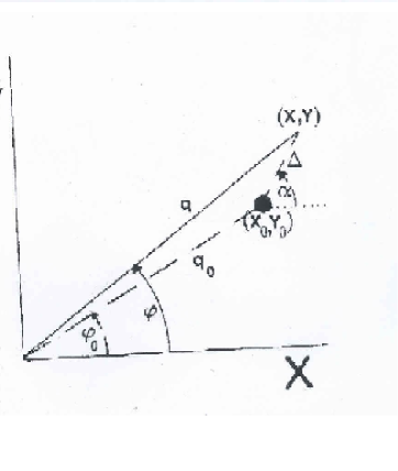
Figure 1: Coordinate systems for the point $(X,Y)$ or $(q,\phi)$ that circles around the point of conical intersection [the dot located at $(X_{0},Y_{0})$ or $(q_{0},\phi_{0})$ ]. The circling is with a radius $\Delta$ and circling angle $\alpha$.

(If $A_{X}=0$, then $A_{Y}$ must be non zero and we use an angle oriented by ${1\over 2}\pi$ from that shown in the drawing.) The introduced quantities are implicitly defined by

$$X-X_{0}=\Delta\cos\alpha,~{}Y-Y_{0}=\Delta\sin\alpha$$ (4)

We now note the important fact that for a ci, in its vicinity, the acquired phase is monotonic with the circling angle and it is therefore permissible to obtain the sign of the phase by looking merely at the limits

$$\alpha\to 0$$ (5)

or, equivalently,

$$\cos\alpha\to 1,~{}~{}\sin\alpha\to\alpha$$ (6)

We thus find for the phase angle, after some elementary simplification,

$$\theta\approx{1\over 2}\arctan(\frac{B_{X}}{A_{X}}+\alpha\frac{A_{X}B_{Y}-B_{X}A_{Y}}{A_{X}^{2}})$$ (7)

with all derivatives to be evaluated at the ci. Since the inverse tangent is an increasing function of it argument, as the circling angle $\alpha$ increases, the mixing angle $\theta$ will increase or decrease depending on whether

$$A_{X}B_{Y}-B_{X}A_{Y}>or<0$$ (8)

(We recall that $A_{X}$ was assumed to be non-zero).

Example 1:

A pair of conical intersections, e.g., (a) in some bent molecules, as $H_{2}S$ of $C_{2v}$ symmetry, two ci’s between the lowest excited states ${}^{1}A_{2}$ and ${}^{1}B_{2}$, (b) for $C_{2}H$ in $C_{s}$ symmetry the $3^{2}A^{\prime}$ and $4^{2}A^{\prime}$ states [13, 14]

We now write out the Hamiltonian representing the coupling between the nuclei, whose coordinates are denoted by $(X,Y)$ and the two electronic states whose surfaces are intersecting conically. For the case of a pair of ci symmetrically situated in the $X,Y$-plane the situation can be described by the following matrix elements:

$$A(X,Y)=(X^{2}-1),~{}B(X,Y)=Y$$ (9)

We have so shifted and scaled the nuclear coordinates, that the ci are located at $X=\pm 1,Y=0$. The representation symbols of Herzberg [15] have been used, for which $X$ transforms in $C_{2v}$ as $B_{2}$, $Y$ as $B_{1}$ and $Z$ as $A_{1}$. We verify that at both ci the partial derivative $A_{X}$ is non vanishing. Furthermore, since

$$A_{X}B_{Y}-B_{X}A_{Y}=2X$$ (10)

has opposite signs for the two ci, we immediately find that the topological angles for the two ci have opposite signs. Therefore, circling around the two ci gives a total accumulated phase of zero, rather than $2\pi$, as might have been expected. This was indeed the result found computationally for large radius circling in some low lying ${}^{2}A^{\prime}$ states in $C_{2}H$ [16]. Thus we conclude that the above model is suitable for this molecule in the vicinity of the ci.

Example 2:

In $C_{2v}$ symmetry the degeneracy between the ${}^{2}B_{2}$ and ${}^{2}A_{1}$ states in $Al-H_{2}$ [3]. Here symmetry arguments forbid the presence of an off diagonal term of the form shown above in equation (9) . Noting further that the ci are in a plane orthogonal to the plane formed by the three atoms, we use $(X,Z)$ instead of $(X,Y)$ and write the off diagonal term as $B(X,Z)$. Terms that are made allowed have the form

$$A(X,Z)=(X^{2}-1),~{}B(X,Z)=XZ$$ (11)

The reason that this off-diagonal term is allowed, is that $X$ transforms as $B_{2}$ and $Z$ as $A_{1}$. The two ci are located at $X={\pm}1,Z=0$. We now find for the Jacobian

$$A_{X}B_{Z}-B_{X}A_{Z}=2X^{2}$$ (12)

and this gives the same sign for either ci. The acquired phase is therefore the same and circling around both yields 2$\pi$.

The results of both Examples 1 and 2 have been previously obtained by us, using a different, graphical-algebraic procedure, the ”continuous phase tracing method” [17].

2.2 Complex representation

This representation is commonly used, e.g. for the doublet electronic states in the $E\otimes\epsilon$ Jahn-Teller problem [18, 2]. The cartesian representation $(X,Y)$ of the nuclear displacement coordinates is conveniently replaced by the cylindrical polar coordinates $(q,\phi)$, according to $X=q\cos\phi,Y=q\sin\phi$. It has been shown [19] that when the vibronic coupling (between nuclear and electronic degrees of freedom) is taken to any arbitrary order, then the matrix in equation (1) (expressing this coupling) can be put in a complex form, such that its off-diagonal part has the form

$$V_{12}(q,\phi)=Kqe^{-i\phi}[1+q^{-2}\sum_{m=1...}q^{3m}Q_{m+}(q)e^{3mi\phi}+\sum_{m=1...}q^{3m}Q_{m-}(q)e^{-3mi\phi}]$$ (13)

Here K is a constant and $Q_{m+}$ and $Q_{m-}$ are polynomials in $q^{2}$ with real coefficients that depend on the physical system (or of the model used to represent it) and whose leading term will be $q^{0}$. (An alternative expression in a real representation is found in [20].) Normally, for stable physical systems, it is expected that with increasing $m$, $Q_{m+}$ and $Q_{m-}$ will both numerically decrease and so will, in each polynomial, the coefficients of successively higher powers of $q^{2}$.

There will also be diagonal, scalar and pseudo-scalar terms. The scalar term simply shifts the energies of the two states by an equal amount and can be ignored. The pseudo-scalar term has the form

$$\sum_{m=1...}q^{3m}P_{m}(q)sin3m\phi$$ (14)

where the polynomials $P_{m}$ are defined in a similar manner to the $Q$’s, above. This term arises when the system is not time-reversal invariant, such as in the presence of a magnetic field. We shall not consider this situation. By consequence, the level separation is simply $2|V_{12}(q,\phi)|$ and the mixing angle is

$$\theta={1\over 2}\arctan\frac{ImV_{12}}{ReV_{12}}$$ (15)

Now, conically intersecting degeneracies of the two (complex) electronic states can occur (those ci are not the only ones possible) at two types of points: At $q=0$, coming from the initial, $q$-factor in equation (13) and at trigonally located degeneracies $(q_{0},\phi_{0})$ from the square-bracket factor in $V_{12}(q,\phi)$, such that one has either

$$\phi_{0}=0,2\pi/3,4\pi/3$$ (16)

or

$$\phi_{0}=\pi/3,\pi,5\pi/3$$ (17)

To find the sign of the phase acquired upon circling around any trigonal ci, we use, as above, the circling radius $\Delta$ and the circling angle $\alpha$ shown in the figure. The polar coordinates, expressed in terms of these are, correct to the first order in $\Delta$,

$$q\approx q_{0}+\Delta\cos(\alpha-\phi_{0}),~{}~{}\\ \phi\approx\phi_{0}+{\frac{\Delta}{q_{0}}}\sin(\alpha-\phi_{0})$$

We shall now find it convenient to rewrite equation (13) in the form

$$V_{12}(q,\phi)=e^{-i\phi_{0}}U_{12}(q,\phi)$$ (18)

where $U_{12}(q,\phi)$ is defined by

$$U_{12}(q,\phi)=Kqe^{-i(\phi-\phi_{0})}[1 + q^{-2}\sum_{m=1...}q^{3m}Q_{m+}(q)e^{3mi\phi}$$ (19)

$$+ \sum_{m=1...}q^{3m}Q_{m-}(q)e^{-3mi\phi}]$$

When this quantity is expanded about the ci, one obtains by equation (2.2)

$$U_{12}(q,\phi)\approx U_{12}(q_{0},\phi_{0})+\Delta cos(\alpha-\phi_{0})(\frac{\partial U_{12}}{\partial q})_{q_{0},\phi_{0}}+\frac{\Delta}{q_{0}}sin(\alpha-\phi_{0})(\frac{\partial U_{12}}{\partial\phi})_{q_{0},\phi_{0}}$$ (20)

The first term on the right vanishes at a point of degeneracy. Real and imaginary parts of $U_{12}(q,\phi)$ come from the middle and the last terms, respectively. Therefore, by equation (15) ,

$$\theta=-i\phi_{0}+{1\over 2}\arctan\Bigl{(}\frac{(\frac{\partial U_{12}}{\partial\phi})_{q_{0},\phi_{0}}}{iq_{0}(\frac{\partial U_{12}}{\partial q})_{q_{0},\phi_{0}}}\tan(\alpha-\phi_{0})\Bigr{)}$$ (21)

The sign of the term linear in the angle $\alpha-\phi_{0}$ will determine the sign of the topological phase.

Example 3: Let us choose, as in an earlier work [10], a quartic approximation for the off-diagonal matrix element

$$V_{12}(q,\phi)=Kqe^{-i\phi}[1-\mu qe^{3i\phi}+\lambda q^{3}e^{-3i\phi}]$$ (22)

We first consider the case in which $\mu$ and $\lambda$ have the same sign. Then, in addition to the zero at the origin, this expression can have up to three sets of trigonally positioned zeros, each of which gives rise to three ci. This is the maximum number of zeros, but since a negative or complex $q_{0}$ is physically not admissible, there may be less than $3\times 3$ ci.

To determine the sign of the phases, one searches for the coefficient in equation (21) of the linear term in $\alpha-\phi_{0}$ as follows: At $q=0$, the coefficient is a constant: $-{1\over{2}}$. This gives, upon full circling, the usual topological phase of $-\pi$. At a trigonal point, one finds for the prefactor of $\alpha-\phi_{0}$

$${\frac{3\mu q_{0}+3\lambda q^{3}_{0}}{\mu q_{0}-3\lambda q^{3}_{0}}}$$ (23)

With the parameters $\lambda$ and $\mu$ having the same sign, the above ratio is positive or negative, depending on whether

$$\sqrt{\frac{\mu}{3\lambda}}>or<q_{0}~{}(the~{}radial~{}position~{}of~{}the~{}{\it ci}~{})$$ (24)

When equality holds, there is a double root and the intersection is no longer conical.

With the choices of $\mu=0.3,\lambda=0.003$ (used for illustration in [10]), the following roots are found:

One root at $q=0$

Further, the following trigonal roots:

$$q_{0}=3.95,\phi_{0}=0,2\pi/3,4\pi/3$$

$$q_{0}=7.42,\phi_{0}=0,2\pi/3,4\pi/3$$

$$q_{0}=11.37,\phi_{0}=\pi,\pi/3,5\pi/3$$ (25)

Substituting the parameter values in the left hand side of the inequalities in equation (24) , one finds for the square root the value of 5.77. This makes the signs of the phase of consecutive sets of ci come out positive, negative and negative (in the order of increasing radius), resulting in accumulated phases of -$\pi$ (around the origin only), then $2\pi$, then -$\pi$ and ultimately, at large radius circling, -$4\pi$. All of these values were confirmed independently by the ”continuous phase tracing method” [10] and by numerical computation of the phase accumulated along the angular coordinate. In the model of [2], and of others ([3], [4] -[6]) identical to that one, the off diagonal matrix element stops with the quadratic term. In the language of our model, exhibited in equation (22) , this means that the coefficient $\lambda$ of the cubic term is zero. In virtue of the criterion expressed in equation (24) this implies a positive phase around each of the three trigonal ci, or for large-radius circling, when the central ci is also circled, a net phase change of +2$\pi$. This agrees with the results of the cited works.

The case of different signs in $\mu$ and $\lambda$ and also $|\frac{\lambda^{\frac{1}{2}}}{2\mu^{\frac{3}{2}}}|<1$ yields three new type of roots, as follows:

$$q_{0}=\sqrt{\frac{-\mu}{\lambda}}$$ (26)

required to be real and positive, with angles $\phi_{0}$ at the intersection that are

$${1\over 3}\arccos[\sqrt{\frac{\lambda}{-\mu}}/(2\mu)]$$ (27)

in which the argument of $\arccos$ is required to be magnitude-wise less than one, as well as two further angles oriented with respect to the previous by $2\pi/3$ and $4\pi/3$. The roots can be checked upon substitution into equation (22) .

The signs of the phase angles can be obtained from equation (15) and equation (20) . After some manipulations one obtains an expression, which reads, correct to the first power of $tan(\alpha-\phi_{0})$,

$$\theta=-{1\over 2}\arctan[{1\over 2}\tan(3\phi_{0})+\frac{3}{4}(\tan(3\phi_{0}))^{2}tan(\alpha-\phi_{0})]$$ (28)

Since $\arctan$ is an increasing function of its argument, and noting the negative sign in the expression, we find that circling around these ci gives a negative phase angle. This last type of ci, which is also trigonally located but angularly shifted from the positions given in equation (16) or equation (17) , has not been noted before, neither experimentally, nor theoretically or calculationally.

2.3 Phases in excited states

(a) A three dimensional parameter space.

The following Hamiltonian was used by Berry [7] for elucidation of the geometric phase in a three-dimensional parameter space represented by ${\bf R}=(X,Y,Z)$. The same Hamiltonian formed the basis of discussion of a magnetic monopole in real space [8].

$$H={1\over 2}\left(\begin{array}[]{cc}Z&X-iY\\ X+iY&-Z\end{array}\right)$$ (29)

This can also be written in terms of Pauli spin matrices, in the form

$$H={1\over 2}(X\sigma_{x}+Y\sigma_{y}+Z\sigma_{z})$$ (30)

The (adiabatic) eigenstates of the Hamiltonian can be obtained in terms of the spherical coordinate representation of ${\bf R}=(R,\theta,\phi)$ as

$$\psi_{l}=\left(\begin{array}[]{cc}-sin\frac{\theta}{2}e^{-i\phi/2}\\ cos\frac{\theta}{2}e^{i\phi/2}\end{array}\right)$$ (31)

for the lower state, and

$$\psi_{u}=\left(\begin{array}[]{cc}cos\frac{\theta}{2}e^{-i\phi/2}\\ sin\frac{\theta}{2}e^{i\phi/2}\end{array}\right)$$ (32)

for the upper (excited) state. The separation of the states is $\Delta=R$. It was shown, in e.g. [9], that the geometric angle $\gamma_{C}$ arising from describing a closed contour $C$ in the $\bf R$- (or parameter) - space can be expressed in terms of the expectation value of gradient of the Hamiltonian

$$\Delta_{\bf R}H={1\over 2}({\bf{\hat{X}}}\sigma_{x}+{\bf{\hat{Y}}}\sigma_{y}+{\bf{\hat{Z}}}\sigma_{z})$$ (33)

namely

$$\gamma_{C}(\psi)=\int_{S}\frac{(\psi|\Delta_{\bf R}H|\psi)}{R^{2}}\cdot d{\bf S}$$ (34)

where the integral is taken over a signed area $\bf S$ enclosed by the contour $C$. Evaluating the expectation values and carrying out the surface integration for a contour at constant $\theta$ (namely, over a region enclosing a spherical cap), one obtains the following geometric phases for the two eigenstates.

$$\gamma_{C}(\psi_{l})=-(1-\cos\theta)\pi$$ (35)

for the lower (ground) state, and its opposite

$$\gamma_{C}(\psi_{u})=(1-\cos\theta)\pi$$ (36)

for the upper (excited) state. One sees that, for a contour around the large circle, for which $\theta={1\over 2}\pi$, the phase-factors, namely $e^{i\gamma_{C}}$, are the same $(-1)$ for the two states, though not the phase-angles, whereas for other values of the angle $\theta$ not even the phase factors are the same. In principle, phase factor differences can be established experimentally by interference measurements.

(b) Adiabatic (slow) time development in a doublet.

We consider the time-dependent Schrödinger equation written as

$$i\frac{\partial\Psi(x,t)}{\partial t}=H(x,t)\Psi(x,t)$$ (37)

(in which $t$ is time, $x$ denotes all particle coordinates, $H(x,t)$ is a real time dependent Hamiltonian and $\hbar=1$). As is well known, the presence of $i$ in the equation causes the solution $\Psi(x,t)$ to be complex-valued. We now consider a special case for the Hamiltonians in which two externally imposed independent sinusoidal perturbation interact linearly with the electron. Further, the electronic Hilbert space is confined to a degenerate electronic doublet, represented by two vectors:$\left(\begin{array}[]{c}1\\ 0\end{array}\right)$ and $\left(\begin{array}[]{c}0\\ 1\end{array}\right)$. In this representation the Hamiltonian can be written as a 2x2 matrix, for which we have chosen the following form, whose physical origin has been described in various works (e.g., [21] - [23])

$$H(t)=G/2\left(\begin{array}[]{cc}-\cos(\omega t)&\sin(\omega t)\\ \sin(\omega t)&\cos(\omega t)\end{array}\right)$$ (38)

Here $\omega$ is the angular frequency of the two external disturbances, taken to be the same for both. The eigenvalues of equation (38) are $-\frac{G}{2}$ and $\frac{G}{2}$. We take $G>0$, so that the former is that ground state energy. A method of solution was outlined in [23] and the amplitude of the vector $\left(\begin{array}[]{c}1\\ 0\end{array}\right)$ in the ground state was given there by the expression

$$\chi_{1}^{g}(t)=\cos(Kt)\cos(\omega t/2)+(\omega/2K)\sin(Kt)\sin(\omega t/2)$$

$$+i(G/2K)\sin(Kt)\cos(\omega t/2)$$ (39)

with

$$K=0.5\sqrt{G^{2}+\omega^{2}}\approx G/2$$ (40)

the latter approximation being justified in the adiabatic, slow motion limit defined by

$$\qquad G/\omega\gg 1$$ (41)

In the present work we do not repeat the method of solution in [23], but use it to present the results also for the amplitude of the vector $\left(\begin{array}[]{c}0\\ 1\end{array}\right)$ for the ground state to be denoted by ${\chi_{2}^{g}(t)}$, as well as the corresponding amplitudes ${\chi_{1}^{e}(t)}$ and ${\chi_{2}^{e}(t)}$ in the excited state. The two states are differentiated by the initial conditions, for $t=0$:

$$\chi_{1}^{g}(0)=1,\chi_{2}^{g}(0)=0$$ (42)

for the ground state and

$$\chi_{1}^{e}(0)=0,\chi_{2}^{e}(0)=1$$ (43)

for the excited state. We recall the well known result that in the adiabatic limit the state maintains its ground or excited state character throughout the motion [24]. After some algebra one obtains the following result, which encapsulates the four amplitudes in one single formula for arbitrary initial values $\chi_{1}(0)$ and $\chi_{2}(0)$:

$$\chi_{{\tiny\left(\begin{array}[]{c}+\\ -\end{array}\right)}}(t) = {\tiny\left(\begin{array}[]{c}1\\ -i\end{array}\right)}\frac{1}{4K}\{e^{i(K-{1\over 2}\omega)t}[\chi_{1}(0)(K+\frac{G}{2}+\frac{\omega}{2})(1{\tiny\left(\begin{array}[]{c}+\\ -\end{array}\right)}f_{1}e^{i\omega t})$$ (50)

$$+ i\chi_{2}(0)(K-\frac{G}{2}+\frac{\omega}{2})(1{\tiny\left(\begin{array}[]{c}-\\ +\end{array}\right)}f_{2}e^{i\omega t})]$$ (53)

$${\tiny\left(\begin{array}[]{c}+\\ -\end{array}\right)} e^{-i(K-{1\over 2}\omega)t}[\chi_{1}(0)(K-\frac{G}{2}+\frac{\omega}{2})(1{\tiny\left(\begin{array}[]{c}+\\ -\end{array}\right)}f_{2}e^{-i\omega t})$$ (58)

$$- i\chi_{2}(0)(K+\frac{G}{2}+\frac{\omega}{2})(1{\tiny\left(\begin{array}[]{c}-\\ +\end{array}\right)}f_{1}e^{-i\omega t})]\}$$ (61)

where the upper and lower symbols in the parentheses have to be taken consistently with the choice of the components. The formula, as presented, is valid generally, for arbitrary boundary conditions. For the special choice of either the ground or the excited state the initial conditions, as expressed in equation (42) or in equation (43) , have to be substituted in the above formula. The auxiliary functions $f_{1}$ and $f_{2}$ are given by

$$f_{1}={{K+\frac{G}{2}-\frac{\omega}{2}}\over{K+\frac{G}{2}+\frac{\omega}{2}}},~{}~{}~{}f_{2}={{K-\frac{G}{2}-\frac{\omega}{2}}\over{K-\frac{G}{2}+\frac{\omega}{2}}}$$ (62)

In the adiabatic limit, when $G/\omega\gg 1$ and therefore $K={1\over 2}\sqrt{G^{2}+\omega^{2}}\approx G/2$ correct to the first order in $\frac{\omega}{G}$, the expression simplifies to take the form:

$$\chi_{{\tiny\left(\begin{array}[]{c}+\\ -\end{array}\right)}}(t) = {\tiny\left(\begin{array}[]{c}1\\ -i\end{array}\right)}\frac{1}{2}\{e^{i(G-{1\over 2}\omega)t}[\chi_{1}(0)(1+\frac{\omega}{2G})(1{\tiny\left(\begin{array}[]{c}+\\ -\end{array}\right)}f_{1}e^{i\omega t})$$ (69)

$$+ i\chi_{2}(0)(\frac{\omega}{2G})(1{\tiny\left(\begin{array}[]{c}-\\ +\end{array}\right)}f_{2}e^{i\omega t})]$$ (72)

$${{\tiny\left(\begin{array}[]{c}+\\ -\end{array}\right)}} e^{-i(G-{1\over 2}\omega)t}[\chi_{1}(0)(\frac{\omega}{2G})(1{\tiny\left(\begin{array}[]{c}+\\ -\end{array}\right)}f_{2}e^{-i\omega t})$$ (77)

$$- i\chi_{2}(0)(1+\frac{\omega}{2G})(1{\tiny\left(\begin{array}[]{c}-\\ +\end{array}\right)}f_{1}e^{-i\omega t})]\}$$ (80)

The crucial element in the establishment of the proper sign of the topological phase is the recognition that the prefactors $f_{1}$ and $f_{2}$ of the circular functions $e^{\pm i\omega t}$ in equation (62) are magnitude-wise less than unity. Therefore, upon circling a full period, none of the round brackets containing these in the above expression can cause a sign change. Thus the sign of the phase is dictated by whether the first or the second term in equation (80) stays finite (non-vanishing) in the adiabatic limit $\frac{\omega}{G}\to 0$. It is now evident from the initial conditions in equation (42) that for the ground state it is the first term that stays finite, and therefore the topological phase is $-\pi$, whereas for the excited state, for which the initial conditions are equation (43) , it is the second term that survives and yields the topological phase of $+\pi$. Note also, that the first exponential factors $e^{{\pm}iGt}$ arise from the dynamical phase and are irrelevant to the topological phase in the adiabatic limit. For their effect upon the topological phase in the not fully adiabatic case, we refer to [25]. We further find from the expression that, in either the ground or the excited state, both components $1$ and $2$ (diferentiated in the above expressions by round and square brackets, respectively) have the same topological phase.

Thus, in summary, we find that the signs of the topological phases are identical for both components in a given state, but are opposite in the ground and excited states. It is possible to interpret this result from a wider perspective, as follows:

The time-dependent ground state of a bound system is characterized by a lower boundedness of the energy. This leads to the analyticity of the wave function (more precisely of its logarithm) in the lower half of the complex t-plane [26, 27]. The phase is then obtained from the modulus by a Kramers-Kronig type relation, which involves integration along a contour consisting of the real t-axis and a large semicircle in the lower half of the t-plane [22, 23, 25]. In contrast, the upper partner in a doublet has an energy upper boundedness. This leads to an analyticity in the upper half t-plane, to a closing of contours (in the Kramers-Kronig relation) in the upper half plane and to a topological phase of the opposite sign.

In a general situation that involves in the Born-Oppenheimer superposition more than two electronic states, one still expects a negatively signed topological phase in the adiabatic ground state, but in general one cannot predict the sign in an intermediate-energy adiabatic state.

3 Pseudo-fields Arising from Degeneracies

Denoting by $|i>$ a set of electronic adiabatic eigenfunctions and by ${\bf\vec{\nabla}}$ the gradient operator conjugate to the nuclear coordinates, we introduce the non-adiabatic coupling terms (NACTs) as

$$\tau_{ij}=<i|{\bf\vec{\nabla}}|j>$$ (81)

It was noted some time ago that the NACTs can be incorporated in the nuclear part of the Schrödinger equationas a vector potential ${\bf A}$ [28]- [32]. The question of a possible magnetic field ${\bf H}$ has been considered in [12] . This field is not due to any source external to the molecule, but rather arises from the mutual coupling between the electrons and the nuclei. To mark this point we call $\bf H$ a pseudo-field. Formally, it is associated with ${\bf A}$ through

$${\bf H}=curl\bf A$$ (82)

In the present work we derive the magnetic field $\bf H$, for the case where the electron- nucleus coupling is expected to have an especial importance, namely, for two (diabatic) electronic states becoming degenerate at a single point in a two dimensional ($2D$) parameter space. In the context of a polyatomic molecule (which is our subject of reference), this $2D$ space is the plane created by a pair of nuclear displacement modes, to be designated $X$ and $Y$. The degeneracy of the electronic states gives rise to a ci, conventionally regarded as the origin $X=Y=0$. The NACTs have a pole at the origin and, excluding this point of singularity but still staying in the neighborhood of the ci , the curl of the NACTs vanishes [34, 35]. Farther away from the ci , the curl of the NACTs is non- vanishing, provided some ci due to other adiabatic states are found in the region. These two facts (the ”vanishing of the curl” around the ci and the existence of a pole at the origin) cause the issue of the magnetic field to be problematic. The approach in this work is to obtain the field associated with the ci by a limiting procedure, which yields the field unambiguously.

The magnetic field that we derive is tied to the fact that in the neighborhood of the ci we have an electronic sub-manifold of at least two dimensions. (The actual electronic Hilbert space is, of course, of higher dimensionality, but this higher dimensionality can be ignored near the ci , whereas a one dimesional space cannot give rise to a ci, by definition.) However, as will be verified in the sequel, the NACT-induced magnetic field will vary with the kind of superposition one makes of the electronic states within the sub-manifold. In the following section we first obtain the magnetic field in the representation of the adiabatic states. These are the appropriate choices under slow variation of nuclear coordinates, since then the adiabatic states are eigen-states which are uncoupled from the rest of the manifold. Subsequently, we shall also consider a magnetic field in another (non-adiabatic) representation. The representation dependence of the magnetic field is connected to the non-Abelian nature of the situation. (”Non-Abelian” means the involvement of more than one electronic state and the presence of non commuting matrices in the Hamiltonian. The need to specify the representation does not arise in Abelian (commuting) systems, which is the usual background for classical electromagnetism. There one defines a unique magnetic field without regard to the electronic state the system is in. The magnetic field is, trivially, ”unique” for a single electronic state. However, it is such also for a many state situation, such that the Hamiltonian contains no non-commuting matrices.)

Another objective of this work is to obtain, in addition to the magnetic field, the tensorial Yang- Mills field. By its original conception [36] and its numerous later developments and applications (e.g., [7] and [38]), the Yang-Mills field constitutes a residual interaction within the manifold (in our context, between the electronic states). From a historical perspective, there is a long and distinguished line of papers in which a magnetic field has been obtained for a related problem: a pair of states that become degenerate at a point in a three dimensional parameter space. Notable among these works are Dirac’s derivations of the quantized monopole- field [39], Wu and Yang’s matched vector potential [40] and Berry’s formulae for the magnetic field (e.g., [7], [41], as are also other papers reprinted in Shapere and Wilczek’s volume [42].)

3.1 The adiabatic states

We start with the following Hamiltonian (taken over from Berry’s ground laying paper [7] with one essential modification)

$$H_{b}=\left(\begin{array}[]{cc}bZ&X-iY\\ X+iY&-bZ\end{array}\right)\qquad\\$$ (83)

This is written in a diabatic representation of the electronic states (that are such that the state does not involve, at least locally, nuclear coordinates). A Hamiltonian matrix written out in a different representation, employed, e.g., in [12] but formally different from that in equation (83) is considered later in this paper. The two components involved in the formalism are denoted by $|+>,|->$, and the nuclear mode coordinates by $(X,Y,Z)(={\bf R})$. The parameter b in equation (83) is to be noted. The magnetic monopole treatment (e.g., in [7, 40]) has $b=1$ and ”spherical symmetry”. We shall obtain the NACT and a magnetic field for a general $b\neq 1$, and then proceed to the $b\to 0$ limit, which is the situation of interest to us, namely the two parameter problem. (The parameter $Z$ varies along the so-called seam-direction of the degeneracies. In the limit of $b=0$, $Z$ does not enter the dynamics. Physically, $bZ$ represents a magnetic field aligned with the quantization direction of the two states in equation (83) . We write it as $\pm bZ$ and then let $b\to 0$, rather than let $Z\to 0$, first to maintain the analogy with [7], and also since a coordinate $Z$ cannot be made to vanish in a Hamiltonian.) The matrix in equation (83) has eigenvalues $\pm R_{b}$ and the corresponding adiabatic states take the form (for $b>0$):

$$|1>=e^{-i\phi/2}\cos(\theta_{b}/2)|+>+e^{i\phi/2}\sin(\theta_{b}/2)|->\\$$ (84)

$$|2>=-e^{-i\phi/2}\sin(\theta_{b}/2)|+>+e^{i\phi/2}\cos(\theta_{b}/2)|->$$ (85)

where

$$R_{b}=\sqrt{X^{2}+Y^{2}+(bZ)^{2}}=\sqrt{q^{2}+(bZ)^{2}}$$ (86)

$$\tan\phi=Y/X\\$$ (87)

$$\tan\theta_{b}=q/bZ$$ (88)

having introduced the radial coordinate $q$ in the cylindrical polar description $(q,\phi)$ through

$$q^{2}=X^{2}+Y^{2}$$ (89)

The NACTs have already been defined as elements of the matrix (denoted by ${\bf\tau}^{b}$) of the gradient operator ${\bf\vec{\nabla}}$ conjugate to the variables $(X,Y,Z)$. Thus ${\bf\tau}^{b}$ is both a vector and a matrix. Its elements in the adiabatic-state representation, equation (84) - equation (85) , are:

$${\bf\tau}^{b}_{11} \equiv <1|{\bf\vec{\nabla}}|1>=-{1\over 2}i\cos\theta_{b}{\bf\vec{\nabla}}\phi$$ (90)

$$= -{\bf\tau}^{b}_{22}$$ (91)

$${\bf\tau}^{b}_{12}={1\over 2}i\sin\theta_{b}{\bf\vec{\nabla}}\phi-{1\over 2}{\bf\vec{\nabla}}\theta_{b}$$ (92)

$${\bf\tau}^{b}_{21}={1\over 2}i\sin\theta_{b}{\bf\vec{\nabla}}\phi+{1\over 2}{\bf\vec{\nabla}}\theta_{b}$$ (93)

[This is a departure from the usual definition in the chemistry literature of NACTs, which are real off-diagonal and anti-symmetric matrices (or matrix elements). However, we shall find that our diagonal NACT are anti-hermitean, just as are the usual NACTs. (Trivially, i times the NACTs are hermitean. The usual definitions of the NACTs can be regained by redefining, say, the second adiabatic state states to be i times the ones used here. Our choice makes the ”off-diagonal” magnetic field, which can be seen below in (16) and (18), come out real.) Particle physicists use the term connectivity ($\bf A$), which also is a matrix-vector, related to $\bf\tau$ by

$${\bf A}=i{\bf\tau}$$ (94)

(as in [37]). They further employ the terms curvature (or the Yang-Mills field intensity tensor), defined by

$${\bf F}={\bf\vec{\nabla}}\wedge{\bf A}-i{\bf A}\wedge{\bf A}={\bf H}-i{\bf A}\wedge{\bf A}$$ (95)

and the Berry-phase or line integral over a closed contour C

$$\int_{C}{\bf A}\cdot d{\bf R}$$ (96)

(The conditions, in a molecular context, for the vanishing of F have been described in [34].)

The magnetic field $\bf H$ arising from the NACTs is

$${\bf H}=i{\bf\vec{\nabla}}\wedge{\bf\tau}$$ (97)

We first calculate this in the representation of the adiabatic states shown in equation (84) -equation (85) .

$${\bf H}^{b}_{11} = -{\bf H}^{b}_{22}=i{\bf\nabla}\wedge{\bf\tau}^{b}_{11}$$ (98)

$$= {1\over 2}{\bf\vec{\nabla}}\wedge(\cos\theta_{b}{\bf\vec{\nabla}}\phi)$$ (99)

$$= -{1\over 2}\sin\theta_{b}({\bf\vec{\nabla}}\theta_{b}\wedge{\bf\vec{\nabla}}\phi)+{1\over 2}\cos\theta_{b}({\bf\vec{\nabla}}\wedge{\bf\vec{\nabla}}\phi)$$ (100)

and

$${\bf H}^{b}_{12} = {\bf H}^{b}_{21}=i{\bf\vec{\nabla}}\wedge{\bf\tau}^{b}_{12}$$ (101)

$$= -{1\over 2}{\bf\vec{\nabla}}\wedge(\sin\theta_{b}{\bf\vec{\nabla}}\phi)$$ (102)

$$= -{1\over 2}\cos\theta_{b}({\bf\vec{\nabla}}\theta_{b}\wedge{\bf\vec{\nabla}}\phi)-{1\over 2}\sin\theta_{b}({\bf\vec{\nabla}}\wedge{\bf\vec{\nabla}}\phi)$$ (103)

having put ${\bf\vec{\nabla}}\wedge{\bf\vec{\nabla}}\theta_{b}=0$ by elementary vector algebra. The (apparently) similar quantity ${\bf\vec{\nabla}}\wedge{\bf\vec{\nabla}}\phi$ needs a different treatment, because of the singular nature of $\phi$ on the seam line $q=0$. This will be done below.

We next calculate the Yang-Mills (tensorial) field, given by

$${\bf F}=i({\bf\vec{\nabla}}\wedge{\bf\tau}+{\bf\tau}\wedge{\bf\tau})={\bf H}+i{\bf\tau}\wedge{\bf\tau}$$ (104)

also in the representation of the adiabatic states

$${\bf F}^{b}_{11} = {\bf H}^{b}_{11}+i{\bf\tau}^{b}_{12}\wedge{\bf\tau}^{b}_{21}$$ (105)

$$= {1\over 2}{\bf\vec{\nabla}}\wedge(\cos\theta_{b}{\bf\vec{\nabla}}\phi)+{1\over 2}\sin\theta_{b}({\bf\vec{\nabla}}\theta_{b}\wedge{\bf\vec{\nabla}}\phi)$$

$$= -{1\over 2}\sin\theta_{b}({\bf\vec{\nabla}}\theta_{b}\wedge{\bf\vec{\nabla}}\phi)+{1\over 2}\cos\theta_{b}({\bf\vec{\nabla}}\wedge{\bf\vec{\nabla}}\phi)$$

$$+ {1\over 2}\sin\theta_{b}({\bf\vec{\nabla}}\theta_{b}\wedge{\bf\vec{\nabla}}\phi)$$ (107)

$$= {1\over 2}\cos\theta_{b}({\bf\vec{\nabla}}\wedge{\bf\vec{\nabla}}\phi)$$ (108)

$$= -{\bf F}^{b}_{22}$$ (109)

and similarly

$${\bf F}^{b}_{12} = {\bf H}^{b}_{12}+i({\bf\tau}^{b}_{11}\wedge{\bf\tau}^{b}_{12}+{\bf\tau}^{b}_{12}\wedge{\bf\tau}^{b}_{22})$$ (110)

$$= -{1\over 2}{\bf\vec{\nabla}}\wedge(\sin\theta_{b}{\bf\vec{\nabla}}\phi)+{1\over 2}\cos\theta_{b}({\bf\vec{\nabla}}\theta_{b}\wedge{\bf\vec{\nabla}}\phi)$$

$$= {1\over 2}\cos\theta_{b}({\bf\vec{\nabla}}\theta_{b}\wedge{\bf\vec{\nabla}}\phi)-{1\over 2}\sin\theta_{b}({\bf\vec{\nabla}}\wedge{\bf\vec{\nabla}}\phi)$$

$$- {1\over 2}\cos\theta_{b}({\bf\vec{\nabla}}\theta_{b}\wedge{\bf\vec{\nabla}}\phi)$$ (112)

$$= -{1\over 2}\sin\theta_{b}({\bf\vec{\nabla}}\wedge{\bf\vec{\nabla}}\phi)$$ (113)

$$= {\bf F}^{b}_{21}$$ (114)

In the above expression we call attention to the cancellation between the terms in the curl and in the vector product (the first and the third terms in equation (107) and equation (112) )

The derivative quantities ${\bf\vec{\nabla}}\phi$ in the NACTs (equation (91) and equation (92) ) and ${\bf\vec{\nabla}}\wedge{\bf\vec{\nabla}}\phi$ in the field intensities (equation (108) and equation (113) ) do not depend on $b$. They have been considered in [32], section III.C in a somewhat different context, namely as arising from a ”pure-gauge” phase factor that multiplies the whole adiabatic state. Their conclusion is that they give rise to a pseudo-magnetic field that is zero everywhere except along the ”curve of intersection [the seam] of the two potential surfaces …where it has a delta-function singularity”. We shall use this result in the formulae that immediately follow, but note that quantities that depend on $b$ are new to the present work and so are some results that do not vanish in the limit of $b\to 0$. (A formal justification of the result of [32] involves the extension of Stokes’ theorem to singular integrands and will be given elsewhere [43].) The $\phi$-derivatives will now be given in two coordinate systems: 1) a cylindrical coordinate system $(q,\phi,Z)$ with unit vectors depicted by bold and hatted symbols and 2) in the Cartesian space $(X,Y,Z)$, for which we quote the results of [32], using the notation of $({\bf i,j,k})$ for the unit orthogonal vectors.

$${\bf\vec{\nabla}}\phi={\bf\hat{\phi}}/q~{}[=(X{\bf j}-Y{\bf i})/(X^{2}+Y^{2})]$$ (115)

$${\bf\vec{\nabla}}\wedge{\bf\vec{\nabla}}\phi={\bf\hat{Z}}\delta(q)/q~{}[=2\pi\delta(X)\delta(Y){\bf k}]$$ (116)

$\delta(q)$ is the Dirac delta function. This result is in accord with [34].

It thus immediately follows that the tensorial fields shown in equation (109) and equation (114) are zero, except on the seam, irrespective of the value of $b$/

3.2 The Non Adiabatic Coupling Terms (NACTs)

The $\sin\theta_{b}$ and $\cos\theta_{b}$ prefactors of these derivatives depend on the parameter $b$, as the notation indicates, and the results are true for any, general value of $b$. However, we shall examine what happens in the $b\to 0$ limit, namely as the 2-parameter (or 2-dimensional) problem is reached. We recall that the angle $\theta_{b}$ has been defined in equation (88) . From this definition, in the limit $b\to 0$, we have, for $q\neq 0$,

$$\lim_{b\to 0}\sin\theta_{b}(=q/R_{b})\to 1~{}~{}(\sin(\frac{\theta_{b}}{2})=\cos(\frac{\theta_{b}}{2})=\frac{1}{\sqrt{2}})$$ (117)

Clearly, also

$$\lim_{b\to 0}\cos\theta_{b}(=bZ/R_{b})\to\pi\delta(q)R_{b}\to\pi\delta(q)q$$ (118)

To obtain the last result we have used the expression for the delta function

$$\pi\delta(q)\ =\lim_{\epsilon\to 0}\frac{\epsilon}{(\epsilon^{2}+q^{2})}$$ (119)

and the definition of $R_{b}$ in equation (86) . We add two further results to be used in the sequel. The first is

$${\bf\vec{\nabla}}\theta_{b}=-(bq/R_{b}^{2}){\bf\hat{Z}}+(bZ/R_{b}^{2}){\bf\hat{q}}~{}[=-(bq/R_{b}^{2}){\bf k}+(bZ/qR_{b}^{2})(X{\bf i}+Y{\bf j})]$$ (120)

and from this, using equation (115) ,

$${\bf\vec{\nabla}}\theta_{b}\wedge{\bf\vec{\nabla}}\phi = (b/R_{b}^{2}){\bf\hat{q}}+(bZ/qR_{b}^{2}){\bf\hat{Z}}$$ (121)

$$[= (b/qR_{b}^{2})(X{\bf i}+Y{\bf j})+(bZ/qR_{b}^{2}){\bf k}]$$ (122)

$$= (bZ/R_{b}^{2})({\bf\hat{q}}/Z+{\bf\hat{Z}}/q)$$ (123)

Then, from equation (90) and equation (115) ,

$${\bf\tau}^{b}_{11} = -{i\over 2}(bZ/qR_{b}){\bf\hat{\phi}}$$ (124)

$$[= -{i\over 2}(bZ/R_{b})(X{\bf j}-Y{\bf i})/(X^{2}+Y^{2})]$$ (125)

$$= -{\bf\tau}^{b}_{22}$$ (126)

$${\bf\tau}^{b}_{12} = {i\over 2}\frac{1}{R_{b}}{\bf\hat{\phi}}-\frac{bZq}{R_{b}^{2}}(\frac{{\bf\hat{q}}}{q}-\frac{{\bf\hat{Z}}}{Z})$$ (127)

$${\bf\tau}^{b}_{21} = {i\over 2}\frac{1}{R_{b}}{\bf\hat{\phi}}+\frac{bZq}{R_{b}^{2}}(\frac{{\bf\hat{q}}}{q}-\frac{{\bf\hat{Z}}}{Z})$$ (128)

From equation (118) we see immediately that (because of the delta function factor arising from $bZ/R_{b}$) the diagonal NACTs are zero outside the seam line $q=0$ as $b\to 0$ . However, on the seam line they are non-zero. This is a new result, which has been obtained by going to the limit $b\to 0$ after calculation of the derivatives.

If we now calculate the Berry-phase or the line integral shown in equation (96) taken with a circular contour encircling the seam line at any finite distance $(q>0)$ from it, we obtain

$$\int_{C}{\bf A}_{11}\cdot d{\bf R}=\pi\cos\theta_{b}$$ (129)

In the 2-parameter limit, as $b\to 0$, this will tend to zero (from equation (118) ). By familiar arguments (based on Stokes’ theorem that equate the contour integral with a surface integral of the curl), the flux across any finite part of the parameters plane of the ”diagonal” magnetic field in the adiabatic representation vanishes, notwithstanding the fact that the vector potential is not zero inside the (infinitely thin) $q=0$ ”solenoid”. (We shall presently check this result by actually calculating the surface integral of the ”diagonal” magnetic field.) In the off-diagonal NACT given in equation (92) or equation (93) , the second term can be seen [from its form in equation (120) ] to give $\delta(q)q$ as $b\to 0$, whose line integral around a finite circle $q>0$ clearly vanishes. However, the first term in the off-diagonal NACTs survives the $b\to 0$ limit even for $q>0$. Thus we have a genuine, finite vector potential entering through the off-diagonal part. The resulting line integral

$$\int_{C}{\bf A_{12}}\cdot d{\bf R}=-\pi\sin\theta_{b}$$ (130)

is responsible for the Berry phase of -$\pi$.

3.3 The magnetic field in the adiabatic representation

As already noted above, we can check the previous line-inegral results by the equivalent method of evaluating the flux of the magnetic field $\bf H$ across an $XY$- plane. $\bf H$ can be calculated from equation (100) and from equation (103) . For the diagonal part we obtain

$${\bf H}^{b}_{11} = [(bZ/2qR_{b})\delta(q)-(bZ/2R_{b}^{2})]{\bf\hat{Z}}-(bq/2R_{b}^{2}){\bf\hat{q}}$$ (132)

$$[= (\pi(bZ/R_{b})\delta(X)\delta(Y)-(bZ/2R_{b}^{3})){\bf k}$$

$$-(b/2R_{b}^{2})(X{\bf i}+Y{\bf j})]$$

$$= -{\bf H}^{b}_{22}$$ (133)

The second expression (in square brackets) is written in the Cartesian frame. In the $b\to 0$ limit this field vanishes outside the seam line $q=0$. In the general case, for which $b>0$ the last term is oriented along the cylindrical radius vector $({\bf q})$ and only the $Z$ component of the field contributes to the flux across the $(q,\phi)$ [or the $(X,Y)$]-plane. Corresponding to the result for a circular contour at $q$ shown in equation (129) which vanishes in the $b\to 0$ limit (as seen above), one obtains after some manipulation of the surface integral

$$\lim_{b\to 0}(Magnetic\ flux)_{11} = \pi\int_{0}^{\infty}dq\delta(q)-\pi bZ\int_{0}^{\infty}dq\frac{q}{R_{b}^{3}}$$ (134)

$$= 0$$ (135)

$$= -(Magneticflux)_{22}$$ (136)

Thus the two methods (the line integral and the surface integration) give the same result.

The off-diagonal magnetic field is from equation (103)

$${\bf H}^{b}_{12} = -{1\over 2}(\frac{\delta(q)}{R_{b}}+\frac{(bZ)^{2}}{qR_{b}^{3}}){\bf\hat{Z}}-{1\over 2}(b^{2}Z/R_{b}^{3}){\bf\hat{q}}$$ (137)

$$[= (-\pi(q/R_{b})\delta(X)\delta(Y)-(bZ)^{2}/2qR_{b}^{3}){\bf k}$$ (139)

$$-(b^{2}Z/2qR_{b}^{3})(X{\bf i}+Y{\bf j})]$$

$$= {\bf H}^{b}_{21}$$ (140)

In the limit $b\to 0$, this field also vanishes outside q=0. To evaluate the flux, care must be taken to go to the limit $b\to 0$ only after the integrations are performed. At the end, one again obtains equation (130) .

3.4 The Yang-Mills fields and collected results

These are defined in equation (104) , are shown for the adiabatic representation in equation (109) - equation (114) ) and have the following forms:

$${\bf F}^{b}_{11} = (bZ/2qR_{b})\delta(q){\bf\hat{Z}}$$ (141)

$$[= (\pi(bZ/R_{b})\delta(X)\delta(Y)){\bf k}]$$ (142)

$$= -{\bf F}^{b}_{22}$$ (143)

and

$${\bf F}^{b}_{12} = -{1\over 2}\frac{\delta(q)}{R_{b}}{\bf\hat{Z}}$$

$$[= -\pi q/R_{b})\delta(X)\delta(Y){\bf k}]$$

$$= {\bf F}^{b}_{21}$$ (145)

These are much simpler than the magnetic (purely curl) field expressions. Their fluxes are given below, in Table 1, where we collect all results in the 2-parameter $b\to 0$ limit.

———————————————————————– ——–

Table 1.Summary for conical intersections in the adiabatic representation in the two-dimensional, $b\to 0$ limit (designated by 0 sub- or super- script.)

Derivatives:${\bf\vec{\nabla}}\phi={\bf\hat{\phi}}/q,{\bf\vec{\nabla}}\theta_{0}=\pi\delta(q){\bf\hat{q}},{\bf\vec{\nabla}}\theta_{0}\wedge{\bf\vec{\nabla}}\phi=\pi\delta(q)({\bf\hat{q}}/Z+{\bf\hat{Z}}/q)$

NACT: ${\bf\tau}^{0}_{11}=-{\bf\tau}^{0}_{22}=-(i/2)\pi\delta(q){\bf\hat{\phi}};{\bf\tau}^{0}_{12}={\bf\tau}^{0*}_{21}={i\over 2}{\bf\hat{\phi}}/q-{1\over 2}\delta(q){\bf\hat{q}}$

Flux or line integrals:

$(Magneticflux)_{11}=-(Magneticflux)_{22}=0$

$(Magneticflux)_{12}=(Magneticflux)_{21}=-\pi$

$(YMflux)11=-(YMflux)22=\pi$

$(YMflux)12=(YMflux)21=0$

———————————————————————– ——–

As already noted, the most remarkable results in Table 1 are the non- zero values of the NACTs upon the seam $q=0$ and the circumstance that the magnetic and Yang-Mills fluxes appear in an opposite manner. These are the legacy of our using the $b\to 0$ limiting procedure, rather than starting with a Hamiltonian in which $b=0$, the $Z$-coordinate is absent and the seam $q=0$ is a line of singularity. The observational significance of the fields or fluxes will be discussed later.

3.5 Circulating representation

In the foregoing, we have calculated the field and the flux on the assumption that the electron is in an adiabatic state. For a slowly changing perturbation, such a state is a stationary state of the system.The diagonal elements of the tensorial quantities that we have calculated refer to this situation. In principle, the electron may be excited to a state different from an adiabatic one, e.g., to a linear combination of two adiabatic states with constant coefficients. The superposition of adiabatic states will persist, since under quasi-stationary conditions each adiabatic state will develop in an independent fashion. The fields pertaining to such a situation can be obtained through use of the non-diagonal elements of the field (or flux), calculated in this work. However, the magnetic field can also react on the electronic motion and this reaction might cause changes in the adiabatic state. This effect is formulated in the last subsection.

We now calculate the fields in a different representation, which we name ”circulating representation” and denote by circularly shaped bras and kets, $|+),|-)$. This is the representation introduced by Baer [12] so as to obtain NACTs that are diagonal (pseudoscalar) and purely imaginary. (It is suggested that in a non-reactive scattering, the $|+),|-)$ states resemble the circulating-state situation.)

The following transformation, acting on the adiabatic states in equation (84) , equation (85) , generates the circulating representation:

$$|+)=[|1>+|2>]/\sqrt{2}$$ (146)

$$|-)=[|1>-|2>]/\sqrt{2}$$ (147)

In the limit $b\to 0$ (where $\sin{\frac{\theta_{0}}{2}}=\cos{\frac{\theta_{0}}{2}}=1/\sqrt{2}$), one has

$$|+)=e^{i\frac{\phi}{2}}|->$$ (148)

$$|-)=e^{-i\frac{\phi}{2}}|+>$$ (149)

where, we recall, $|->$ and $|+>$ are diabatic coordinate independent electronic states. The complex exponential prefactor is the reason for the name ”circulating representation”. [When $b$ is non-zero, the circulating states are coordinate dependent superpositions of the diabatic states.] We list the results in this representation, obtained after using some algebra:

———————————————————————– ——–

Table 2. Results in the circulating representation with the arrow denoting the $b\to 0$ limit:

NACTs:

${\bf\tau}^{b}_{++}=\frac{i{\bf\hat{\phi}}}{2R_{b}}\to\frac{i{\bf\hat{\phi}}}{2q}$

${\bf\tau}^{b}_{--}=-\frac{i{\bf\hat{\phi}}}{2R_{b}}$

${\bf\tau}^{b}_{-+}=-\frac{i{bZ{\bf\hat{\phi}}}}{2qR_{b}}-{1\over 2}\frac{bZ}{R_{b}^{2}}{\bf\hat{q}}+{1\over 2}\frac{bq{\bf\hat{Z}}}{R_{b}^{2}}$

${\bf\tau}^{b}_{+-}=-\frac{i{bZ{\bf\hat{\phi}}}}{2qR_{b}}+{1\over 2}\frac{bZ}{R_{b}^{2}}{\bf\hat{q}}-{1\over 2}\frac{bq{\bf\hat{Z}}}{R_{b}^{2}}$

Fluxes or line integrals, for $b\to 0$:

$(Magneticflux)_{++}=-(Magneticflux)_{--}\to-\pi$

$(Magneticflux)_{+-}=(Magneticflux)_{-+}\to 0$

$(YMflux)_{++}=-(YMflux)_{--}\to 0$

$(YMflux)_{+-}=(YMflux)_{-+}\to\pi$

———————————————————————– ——–

We note that for $b$ nonzero the NACTs have also off-diagonal elements and that on the seam $q=0$ these elements exist even in the two-dimensional limit $b\to 0$. Moreover, these elements have components other than tangential (along ${\bf\hat{\phi}})$. As such, they do not contribute to the line integral in equation (96) . At finite distances from the seam $q>0$, our results agree with those in [12].

3.6 An alternative formalism

Our results could also have been obtained, had we proceeded differently, namely by making the $X$ and $Z$ the ”active” variables and $Y$ the fictitious one. To achieve this one puts the $b$ factor (whose limit 0 is ultimately taken) in front of $Y$ in the Berry Hamitonian, our equation (83) , rather than before $Z$. This amounts to a representation of the diabatic electronic states that is obtained from the $|+>,|->$ set used above, by a complex transformation. In the $b\to 0$ limit the adiabatic states are the same in either formalism and so are the NACTs and the magnetic field. An historical interest is attached to the latter procedure in that Stone not only proposed this Hamiltonian [46], with the interpretation of $b$ as a spin orbit coupling strength, but even considered the limit of $b\to 0$ . However, he did not derive a magnetic field.

3.7 General linear coupling and derived quantities

The most general form for the interaction Hamiltonian that is linear in the parameters $(X,Y,Z)$ is the following:

$$H_{b}=\left(\begin{array}[]{cc}bZ&\alpha X-i\beta Y\\ \alpha X+i\beta Y&-bZ\end{array}\right)\qquad\\$$ (150)

This differs from equation (83) by the inequivalence between not only $Z$ (for $b\neq 1$) and $X,Y$, but also between $X$ and $Y$. One regains the formalism of [47], upon using the substitutions $b=0,\alpha\to b,\beta\to 1$. In this two-dimensional (or two-parameter) case the intersection between the two adiabatic potential surfaces (the solution of equation (150) ) involves two inverted elliptic cones, rather than two inverted circular ones which one obtains for $b=0,\alpha=\beta$. The method of the previous section can be easily carried over to this case and we shall only quote the modifications needed for the generalization. Our main purpose is to demonstrate explicitly the dependence of the magnetic and Yang-Mills fields on the angle $\phi$ defined in equation (87) . A dependence of this type has been predicted in [12]. We first define

$$\gamma=\alpha/\beta$$ (151)

so that $\gamma=1,\beta=1$ takes us back to the previous sections. Otherwise, (when $\gamma\neq 1$)we have the following modifications, designated by placing an apostrophe over all symbols affected:

The adiabatic states have now the following form:

$$|1^{\prime}>=e^{-i\phi^{\prime}/2}\cos(\theta^{\prime}_{b}/2)|+>+e^{i\phi^{\prime}/2}\sin(\theta^{\prime}_{b}/2)|->\\$$ (152)

$$|2^{\prime}>=-e^{-i\phi^{\prime}/2}\sin(\theta^{\prime}_{b}/2)|+>+e^{i\phi^{\prime}/2}\cos(\theta^{\prime}_{b}/2)|->$$ (153)

where

$$R^{\prime}_{b}=\sqrt{(\alpha X)^{2}+(\beta Y)^{2}+(bZ)^{2}}=\sqrt{q^{\prime 2}+(bZ)^{2}}$$ (154)

$$tan\phi^{\prime}=\beta Y/(\alpha X)$$ (155)

$$tan\theta^{\prime}_{b}=q^{\prime}/bZ$$ (156)

having introduced the modified radial cylindrical coordinate $q^{\prime}$ through

$$q^{\prime 2}=(\alpha X)^{2}+(\beta Y)^{2}$$ (157)

The NACTs are now

$$\bf\tau^{{}^{\prime}b}_{11} \equiv <1^{\prime}|\vec{\nabla}|1^{\prime}>=-{i\over 2}\cos\theta^{\prime}_{b}\vec{\nabla}\phi^{\prime}$$ (158)

$$= -\bf\tau^{{}^{\prime}b}_{22}$$ (159)

$${\bf\tau}^{{}^{\prime}b}_{12}={1\over 2}i\sin\theta^{\prime}_{b}\vec{\nabla}\phi^{\prime}-{1\over 2}\vec{\nabla}\theta^{\prime}_{b}$$ (160)

$${\bf\tau}^{{}^{\prime}b}_{21}={1\over 2}i\sin\theta^{\prime}_{b}\vec{\nabla}\phi^{\prime}+{1\over 2}\vec{\nabla}\theta^{\prime}_{b}$$ (161)

The derivatives of the angles are

$${\bf\vec{\nabla}}\phi^{\prime}=\frac{\gamma}{1+(\gamma^{2}-1)\cos^{2}\phi}{\bf\hat{\phi}}/q=\frac{\alpha\beta}{q^{{}^{\prime}2}}q{\bf\hat{\phi}}$$ (162)

$${\bf\vec{\nabla}}{\bf\wedge\vec{\nabla}}\phi^{\prime}=\frac{\gamma}{1+(\gamma^{2}-1)\cos^{2}\phi}\frac{\delta(q)}{q}{\bf{\hat{Z}}}=\frac{\alpha\beta}{q^{{}^{\prime}2}}q\delta(q){\bf\hat{Z}}$$ (163)

$${\bf\vec{\nabla}}\theta^{\prime}_{b}=-(bq^{\prime}/R_{b}^{{}^{\prime}2}){\bf\hat{Z}}+(bZ/R_{b}^{{}^{\prime}2})\frac{q^{\prime}}{q}{\bf\hat{q}}-\frac{bZq}{2q^{\prime}R_{b}^{{}^{\prime}2}}(\alpha^{2}-\beta^{2})\sin 2\phi{\bf\hat{\phi}}$$ (164)

and

$${\bf\vec{\nabla}}\theta^{\prime}_{b}\wedge{\bf\vec{\nabla}}\phi^{\prime}=\frac{bZ}{R_{b}^{{}^{\prime}2}}\frac{\alpha\beta q}{q^{\prime}}({\bf\hat{q}}/Z+{\bf\hat{Z}}/q)$$ (165)

In equation (164) the last term is new. In the adiabatic representation equation (152) and equation (153) one finds the following NACTs

$${\bf\tau}^{{}^{\prime}b}_{11} = -{i\over 2}(bZ/qR^{\prime}_{b})\frac{\gamma}{1+(\gamma^{2}-1)\cos^{2}\phi}{\bf\hat{\phi}}$$ (166)

$$= -{\bf\tau}^{{}^{\prime}b}_{22}$$ (167)

and

$${\bf\tau}^{{}^{\prime}b}_{12} = \big{(}\frac{i\alpha\beta}{2R^{\prime}_{b}}+(\alpha^{2}-\beta^{2})\sin 2\phi\frac{bZ}{4R^{{}^{\prime}2}_{b}}\big{)}\frac{q}{q^{\prime}}{\bf\hat{\phi}}-\frac{bZq^{\prime}}{2R_{b}^{{}^{\prime}2}}(\frac{{\bf\hat{q}}}{q}-\frac{{\bf\hat{Z}}}{Z})$$ (168)

$${\bf\tau}^{{}^{\prime}b}_{21} = \big{(}\frac{i\alpha\beta}{2R^{\prime}_{b}}-(\alpha^{2}-\beta^{2})\sin 2\phi\frac{bZ}{4R^{{}^{\prime}2}_{b}}\big{)}\frac{q}{q^{\prime}}{\bf\hat{\phi}}+\frac{bZq^{\prime}}{2R_{b}^{{}^{\prime}2}}(\frac{{\bf\hat{q}}}{q}-\frac{{\bf\hat{Z}}}{Z})$$ (169)

In the two parameter limit $b\to 0$ for non-zero $q$ the only term remaining is

$${\bf\tau}^{{}^{\prime}0}_{12} = {\bf\tau}^{{}^{\prime}0}_{21}$$ (170)

$$= \frac{i\alpha\beta}{2R^{\prime}_{b}}\frac{q}{q^{\prime}}{\bf\hat{\phi}}$$ (171)

$$= {i\over 2}\frac{\gamma}{1+(\gamma^{2}-1)\cos^{2}\phi}\frac{{\bf\hat{\phi}}}{q}$$ (172)

The off-diagonal coupling term obtained in [13] computationally for the molecule $C_{2}H$ near a conical intersection was subsequently fitted to the above expression in equation (172) [47]. The coupling term is characterized (for $\gamma<1)$by two (frequently quite dominant) peaks at $\phi=0(=2\pi)$ and $\pi$. However, on the seam $q=0$ there are additional non-zero terms in ${\bf\tau}^{{}^{\prime}0}_{12}$, in ${\bf\tau}^{{}^{\prime}0}_{11}$, etc., as we have already noted. These are new results. One expects similar angular behavior from them, too. The line integral over the coupling coefficient, or the Berry phase, in equation (96) gives in the $b\to 0$ limit the values of 0 for the diagonal terms and $\pm\pi$ for the off diagonal terms, irrespective of the value of the ratio $\gamma=\alpha/\beta$. These values were confirmed numerically to a good approximation for the neighborhood of the intersection in [13] and discussed in [47].

Returning to general values of the parameters $b,\alpha,\beta,$ we show now the fields (magnetic and Yang-Mills):

$${\bf H}^{{}^{\prime}b}_{11} = \alpha\beta[\frac{bZ}{2R_{b}^{{}^{\prime}2}}(\frac{qR^{\prime}_{b}}{q^{{}^{\prime}2}}\delta(q)-\frac{1}{R^{\prime}_{b}}){\bf\hat{Z}}-(bq/2R_{b}^{{}^{\prime}3}){\bf\hat{q}}]$$ (173)

$$= -{\bf H}^{{}^{\prime}b}_{22}$$ (174)

$${\bf H}^{{}^{\prime}b}_{12} = -\alpha\beta[(\frac{q\delta(q)}{2q^{\prime}R^{\prime}_{b}}+\frac{(bZ)^{2}}{2q^{\prime}R_{b}^{{}^{\prime}3}}){\bf\hat{Z}}-\frac{b^{2}Z}{2R_{b}^{{}^{\prime}3}}\frac{q}{q^{\prime}}{\bf\hat{q}}]$$ (175)

$$= {\bf H}^{{}^{\prime}b}_{21}$$ (176)

In the limit $b\to 0$, this field also vanishes outside $q=0$. However, on the seam $q=0$ we obtain one of the interesting results of this section, namely the angular dependence of the magnetic field. Only the second term in equation (175) for ${\bf H}^{{}^{\prime}b}_{12}$ survives in this limit and one obtains after a slight simplification

$${\bf H}^{{}^{\prime}0}_{12}=-{1\over 2}\frac{\gamma\delta(q)}{1+(\gamma^{2}-1)\cos^{2}\phi}{\bf\hat{Z}}$$ (177)

An angular dependence of the seam magnetic field was postulated in [12]. The above relation gives its form within the general (elliptic) linearly dependent model. The total flux in the $b\to 0$ limit is again the limiting form of equation (130) , namely $-\pi$.

The Yang Mills tensorial fields are calculated as:

$${\bf F}^{{}^{\prime}b}_{11} = \alpha\beta\frac{bZq\delta(q)}{2q^{{}^{\prime}2}R^{\prime}_{b}}{\bf\hat{Z}}$$ (178)

$$= -{\bf F}^{{}^{\prime}b}_{22}$$ (179)

whose integrated flux in the $b\to 0$ limit is $\pi$ for all values of $\alpha$ and $\beta$ . Finally,

$${\bf F}^{{}^{\prime}b}_{12} = -\alpha\beta\frac{q\delta(q)}{2q^{\prime}R_{b}}{\bf\hat{Z}}$$ (180)

$$= {\bf F}^{{}^{\prime}b}_{21}$$ (181)

whose flux is 0 for all finite values of $b$. Since in our limiting procedure the limit $b\to 0$ is taken at the end, we have a zero flux in the two-dimensional elliptic geometry, which is identical to the entry in Table 1 for the circular case.

3.8 Interpretation of the fields

Associated with a ci of two potential surfaces for a polyatomic molecule, there exists an analogue of a magnetic field, which affects the nuclear motion through its presence in the nuclear Schrodinger equation. However, in addition to the magnetic field, there is an analogous, symmetry-based field, the Yang-Mills or tensorial field. By employing a limiting procedure we have shown that for a (multiple valued) adiabatic state both types of the field have delta-function-like, thin solenoidal forms.

In the molecular context, the direction of the solenoid is defined by the ci, as follows: The ci defines a plane in the nuclear coordinate space; the direction of the field is along any arbitrary direction in the nuclear coordinate space (the ”seam”), which is perpendicular to this plane. Though the two types of fields have similarities, they differ in their numerical values and the fluxes due to them ”complement” each other (Tables 1 and 2). We have also found that the fluxes are quantized, meaning that the strength of the field and the flux associate with it do not depend on physical parameters, just as they don’t for the magnetic monopole field of Dirac [39]. This result was obtained recently [12], where the ”curl- field” was calculated by applying a complex-valued linear superposition of the adiabatic states. This superposition is equivalent to that introduced here for a pair of circulating states (one clockwise and another anti-clockwise) around the seam. It also expresses the geometry of the Aharonov-Bohm effect, in which two currents circle around a screened solenoid in opposite senses. However, in that case the flux is not quantized, but depends on the magnetic field inside the solenoid.

As noted above, the ”curl-field” is a delta function along the seam, so that a particle circulating at a finite radius would be oblivious of this field. A different situation could arise when the electron is excited into a general superposition state, i.e. one that is not a superposition of adiabatic states (or is a superposition thereof, but with coefficients depending on the coordinates.) The ”magnetic field” would be completely different from those for the adiabatic states. Formally, the new, general superposition would be described by applying what is called a ”non-local” gauge transformation [37, 38]. The effect of this is well known and is expressed by saying that the vector potentials $\bf A$ (or the NACTs) transform inhomogeneously and the tensorial field $\bf F$ does so homogeneously in a covariant way [37]. However, for a coordinate dependent superposition, the fields may be difficult observe (if at all possible), due to the off-diagonal matrix elements in the potential, which make such a state non-stationary.

3.9 Observational aspects through effective Hamiltonians

Possible experimental consequences of gauge fields have been noted for electron spin experiments with time-varying magnetic fields [48], in atoms with rotating electric fields [48], in collisions between atoms [30] and in further applications [42].

We now give a general formalism for the observational effects of the fields, one that holds the promise of differentiating between the magnetic and the Yang-Mills field. It is based on an effective or truncated Hamiltonian formalism, similar in many respects to the well known Spin-Hamiltonian description ([49] -[51]). This concentrates on a small set of states (in the present context, the two-fold set in equation (84) and equation (85) ), and considers the effects of perturbations on these. The perturbations admix states from outside the small set. The Spin-Hamiltonian formalism shows a way to represent the effect of the full set within the small (”truncated”) set, in such a manner that the excited electronic states are included only ”virtually”. Symmetry considerations determine the form of the truncated Hamiltonian. Clearly, since several independent expressions can be compatible with the symmetry requirement, as e.g., by including higher order effects, the effective Hamiltonian will normally consist of several terms. The coefficients with which these terms enter will in general not be amenable to calculations, but are empirically determined.

After these preliminary remarks we recall that the previous subsections treated electronic and nuclear degrees of freedom. The fields that we have derived were pseudo-vector quantities in the nuclear space and were functions of the nuclear variables $(X,Y,Z)$ or $(q,\theta,\phi)$. Moreover, the fields were elements of a matrix (or tensor) in the Hilbert space of the electronic set, which is not the case in ordinary electromagnetism. We shall write a generic field component (not differentiating for the moment between magnetic and Yang-Mills fields) as

$$F^{a}_{mn}=F^{a}_{mn}(X,Y,Z)$$ (182)

where $a$ is the vector-index in the nuclear coordinate space and $(m,n)$ are labels for the electronic set. We shall also consider operators of two types. First, the operators

$$op^{a}_{1},op^{ab}_{2},etc.$$ (183)

in the nuclear vector-space that are functions of electronic variables. It is now elementary to construct terms for an effective Hamiltonian $H_{eff}$, such that satisfy the symmetry requirements:

$$H_{eff}=|m>(C_{1}F^{a}_{mr}<r|op^{a}_{1}|n>+C_{2}F^{a}_{mp}F^{b}_{pr}<r|op^{ab}_{2}|n>+...)<n|$$ (184)

with possible additional terms to follow. Summation for repeated indexes is implied. The first operator $op^{a}_{1}$ is a pseudo-scalar and the second operator $op^{ab}_{2}$ has also the appropriate transformation properties.(Thus it might be a direct product of two $op^{a}_{1}$’s.) The coefficients $C_{1},C_{2},etc.$ are expected to be empirical parameters.

As a second application we consider the extension of the electronic (orbital) degrees of freedom, e.g., by inclusion of electronic spins. We label the set for the extended degree of freedom by $|M>$ and operators that act on both the electronic orbital and spin degrees of freedom by $Op^{a}_{1},Op^{ab}_{2}$, etc. The $a,b$ indexes refer to the axes in nuclear space, as before. Then the effective Hamiltonian takes the following form:

$$H_{eff}=|m>|M>(C_{1}F^{a}_{mr}<r|<M|Op^{a}_{1}|n>|N>$$

$$+C_{2}F^{a}_{mp}F^{b}_{pr}<r|<M|Op^{ab}_{2}|n>|N>+...)<n|<N|$$ (185)

Evaluation of these Hamiltonians requires computing expectation values in a given nuclear state. Since $H_{eff}$ is anticipated to be small compared to energies of the nuclear freedom, this is a legitimate procedure. The effective Hamiltonian thus provides a way to include residual perturbations that couple to states outside the degenerate electronic doublet. We have seen above (e.g. in Tables 1 and 2) that the magnetic field and the Yang- Mills field differ markedly. It is therefore suggested that by experimentally testing the effective Hamiltonian (e.g., through its dependence on the nuclear vibrational levels) one could establish which field is effective.

4 Conclusion

This paper explains the signs of topological phases obtained by various authors in several previous works. The sign depends on the derivatives of the coupling matrix and is shown by the inequalities in equation (8) for a cartesian, real representation and in equation (21) for a complex representation. Although positively and negatively signed topological phases cannot be distinguished, since they have the same phase factor, this is true only upon performing a complete loop. For loops shorter or longer that this, the sign of the phase change is observationally accessible.

We then obtain for various models the state- or representation- dependent magnetic and Yang-Mills fields, which result from the Born - Oppenheimer scheme for the coupling between nuclear and electronic degrees of freedom. An effective or truncated Hamiltonian, here suggested, provides a possible tool for experimental verification of the fields.

5 Figure Caption

Figure 1.

Coordinate systems for the point $(X,Y)$ or $(q,\phi)$ that circles around the point of conical intersection [the dot located at $(X_{0},Y_{0})$ or $(q_{0},\phi_{0})$ ]. The circling is with a radius $\Delta$, and circling angle $\alpha$.

References

- [1] H.C. Longuet-Higgins, Proc. Roy. Soc. (London) A 344 147 (1975)
- [2] J.W.Zwanziger and E.R. Grant, J. Chem. Phys. 87 2954 (1987)
- [3] D. Yarkony, Acc. Chem. Res. 31 511 (1998)
- [4] H. Koppel and R. Meiswinkel, Z. Physik D 32 153 (1994)
- [5] D. Yarkony, J. Chem. Phys. 111 906 (1999)
- [6] H. Koizumi and I.B. Bersuker, Phys. Rev. Lett. 83 3009 (1999)
- [7] M.V. Berry, Proc. Roy. Soc. London A392 45 (1984)
- [8] T.T. Wu and C.N. Yang, Phys. Rev. D 12 3845 (1975)
- [9] M.S. Child, Geometric Phase in Molecular Systems Lecture Notes in the ”Charles Coulson Summer School on the Quantum Dynamics of Molecular Systems” (Oxford, 15 August 2001)
- [10] R. Englman and A. Yahalom, Adv. Chem. Phys. 124 197 (2002)
- [11] S. Matsika and D.R. Yarkony, J. Chem. Phys. 115 5066 (2001); 115 5066 (2001);116 2825 (2002)
- [12] M. Baer, Chem. Phys. Lett. 349 84 (2001)
- [13] A.M. Mebel, M. Baer and S.H. Lin, J. Chem. Phys. 112 10 703 (2000)
- [14] A.M. Mebel, M. Baer and S.H. Lin, J. Chem. Phys. 114 5109 (2001)
- [15] G. Herzberg, Molecular Spectra and Molecular Structure (Van Nostrand, Princeton, 1966 ) Vol. 3
- [16] A.M. Mebel, A. Yahalom, R. Englman and M. Baer, J. Chem. Phys. 115 3673(2001)
- [17] R. Englman, A. Yahalom, M. Baer and A.M. Mebel, Int. J. Quant. Chem. (to appear)
- [18] R. Englman, The Jahn-Teller Effect in Molecules and Crystals (Wiley, Chichester, 1972)
- [19] R. Englman and A. Yahalom, Adv. Chem. Phys. 124 197 (2002)
- [20] T.C. Thompson and C.A. Mead, J. Chem. Phys. 82 2408 (1985)
- [21] D.J. Moore and G.E. Stedman, J. Phys. A 23 2049 (1990)
- [22] R. Englman and A. Yahalom, Phys. Rev. A 60 1802 (1999)
- [23] R. Englman, A. Yahalom and M. Baer, Eur. Phys. J. D 8 1 (2000)
- [24] M. Born and V. Fock, Z. Phys. 51 165 (1928)
- [25] R. Englman, A. Yahalom and M. Baer, Phys. Letters A 251 223 (1999)
- [26] L. A. Khalfin, Soviet Phys. JETP 6 1053 (1958)
- [27] M. E. Perel’man and R. Englman, Mod. Phys. Lett. B 14 907 (2000)
- [28] F.T. Smith, Phys. Rev. 179 111 (1969)
- [29] C.A. Mead, Phys. Rev. Lett. 59 161 (1987)
- [30] B. Zygelman, Phys. Lett. A 125 476 (1987)
- [31] Y. Aharonov, E. Ben-Reuven, S. Popescu and D. Rohrlich, Nucl. Phys. B350 818 (1991)
- [32] C.A. Mead and D.G. Truhlar, J. Chem. Phys. 70 2284 (1979)
- [33] J. Avery, M. Baer and G.D. Billing, Mol. Phys. 100 1011 (2002)
- [34] M. Baer, Chem. Phys. Lett. 35 112 (1975)
- [35] M. Baer, Phys. Repts. 358 75 (2002)
- [36] C.N. Yang and R. Mills, Phys. Rev. 96 191 (1954)
- [37] R. Jackiw, Rev. Mod. Phys. 52 661 (1980)
- [38] S. Weinberg, The Quantum Theory of Fields (University Press, Cambridge 1996) Vol. 2, Chapter 15
- [39] P.A.M. Dirac, Proc. Roy. Soc. London A 133 60 (1931)
- [40] T.T. Wu and C.N. Yang, Phys. Rev. D 12 3845 (1975)
- [41] M.V. Berry in A.Shapere and F. Wilczek (Editors), Geometrical Phases in Physics (World Scientific, Singapore, 1989) p. 7
- [42] A. Shapere and F. Wilczek (Editors), Geometrical Phases in Physics (World Scientific, Singapore, 1989)
- [43] A. Yahalom and R. Englman, Corrections to Stokes’ Theorem for Singular Integrands (to be published)
- [44] D. Suter, K.T. Mueller and A. Pines, Phys. Rev. Lett. 60 1218 (1988)
- [45] S. Fuentes-Guridi, S. Bose and V. Vedral, Phys. Rev. Lett. 85 5018 (2000)
- [46] A.J. Stone, Proc. Roy. Soc. London A351 141 (1976)
- [47] M.Baer, A.M. Mebel and R. Englman, Chem. Phys. Lett. 354 243 (2002)
- [48] J. Moody, A. Shapere and F. Wilczek, Phys. Rev. Lett. 56 893 (1986)
- [49] M.H.L. Pryce, Proc. Phys. Soc.(London) 63 25 (1950)
- [50] W.K.H. Stevens, Rep. Prog. Phys. 30 189 (1967), Magnetic Ions in Crystals (Princeton University Press, Princeton, N.J., 1997) Chapter 7
- [51] A. M. Stoneham, The Theory of Defects in Solids (Clarendon Press, Oxford, 1975) Chapter 13