When is the two-level approximation untenable in issues of Decoherence?

Abstract

We examine the conditions in favor and necessity of a realistic multileveled description of a decohering quantum system. Under these conditions approximate techniques to simplify a multileveled system by its first two levels is unreliable and a realistic multilevel description in the formulation of decoherence is unavoidable.

In this regard, our first crucial observation is that, the validity of the two level approximation of a multileveled system is not controlled purely by sufficiently low temperatures. We demonstrate using three different environmental spectral models that the type of system-environment coupling and the environmental spectrum have a dominant role over the temperature. Particularly, zero temperature quantum fluctuations induced by the Caldeira-Leggett type linear coordinate coupling can be influential in a wide energy range in the systems allowed transitions. The second crucial observation against the validity of the two level approximation is that the decoherence times being among the system’s short time scales are found to be dominated not by the resonant but non-resonant processes. We demonstrate this in three stages. Firstly, our zero temperature numerical calculations reveal that, the calculated decoherence rates including relaxation, dephasing and leakage phenomena show, a linear dependence on the spectral area for all spectral models used, independent from the spectral shape within a large environmental spectral range compared to the quantum system’s energies. Secondly, within the same range, the decoherence times only have a marginal dependence on the translations of the entire frequency spectrum. Finally, the same decoherence rates show strong dependence on the number of coupled levels by the system-environment coupling.

I Introduction

The nature of the environmental coupling and the properties of the environmental spectrum are essential factors in the determination of the decoherence properties of multileveled quantum systems (MLS). Most of the realistic MLS have Caldeira-Leggett type linear couplingCL ; LG of a macroscopic system coordinate to an external environmental noise field. In this publication, the MLS is identified by a large number of energy levels coupled by non-negligible matrix elements induced by an environmental perturbation. The first two levels comprise the non ideal qubit space which we consider to be energetically well separated from the higher levels. The analysis of the decoherence properties of such MLS has recently appeared in a few publicationsTS1 ; DiVinc .

Normally a physical environmental spectrum (the so called noise) has a large range of frequencies with different characteristic behavior in different spectral regions. Moreover, the spectral noise range usually extends well beyond the energy scales of the quantum system that it interferes with. In most of the environmental models, weak noise signals and a realistic linear coupling suffices to model the system-noise interference. On the other hand, it is customary to consider the decohering quantum system as a two level approximated version of a generic MLS. The well studied spin-bosonSB1 ; SB2 or central spinSBCS models are such examples arising from the assumption that for sufficiently low temperatures $T\ll\Delta E$ a MLS is well approximated by its first two levelsSB1 (where $\Delta E$ is a characteristic energy scale separating the first two levels from the higher excited states of the quantum system). This two level approximation (2LA) has in its essence three assumptions: a) that the incoherent transitions caused by the environment in the system are generated by the resonant processes: Implicit in the 2LA is the belief that the spectrum must have non-negligible couplings at the right transition frequencies at which the system makes transitions to higher levels. b) at zero or sufficiently low temperatures there are no available environmental states to couple with the system: This assumption and the notion of the right transition frequency basically help to neglect all parts of the spectrum $\Delta E\leq\omega$ because of the religious belief that at sufficiently low temperatures the relevant part of the spectrum is the low energy sector $\omega\leq T\ll\Delta E$ of which coupling is suppressed by thermal considerations. c) negligible leakage of the wave-function to higher levels: In fact these effects have not been seriously questioned until recently. Contrary arguments to the negligible leakage can be found for instance in the recent publication Ref.[DiVinc ].

This manuscript presents counter arguments to these three fundamental assumptions of the 2LA mentioned above by considering a MLS interacting with a bosonic environmental bath at zero temperature through a Caldeira-Leggett type linear coordinate coupling. By considering a spectral noise range extending well beyond the thermal and the system energy scales, and adopting a model MLS for which $T\ll\Delta E$ is well satisfied we demonstrate that the three basic assumptions of the 2LA are neither necessary nor sufficient for its validity.

The method that we employ is the direct numerical solution of the master equation for the multileveled quantum systems’ reduced density matrix (RDM) in the short-time Born-Oppenheimer approximation. That the calculated decoherence rates are largely independent from where the energy levels are, is demonstrated. This observation of the independence of the decoherence rates from the location of the resonant transition energies provides the first clue of the strong influence of the non-resonant processes. The main results are two fold: i) Decoherence is dominated by the non-resonant processes at zero temperature implying that decoherence times are finite and saturate near zero temperature: This observation basically invalidates the assumption (a) above. ii) In a realistically multileveled system, and following (i), non-resonant processes induced in the entire environmental spectral range additionally cause wave-function leakage from the qubit subspace to the system’s higher levels. Our numerically calculated leakage (L) times are in the same order of magnitude as the relaxation/dephasing (RD) times. Therefore the leakage, being a characteristic MLS effect, renders itself to be non-negligible at short times. The observation of strong leakage at short times invalidates the conventional belief that the affect of multilevels in decoherence is a mere renormalizion of the effective two level system parameters.

The zero temperature quantum fluctuations of the model system in (1) are caused by the system-environment coupling in which the number of excitations in the environmental modes is unconserved by the interaction. Decoherence is caused by the participation of large number of these modes in the interaction. Similar zero temperature decoherence mechanisms have been recently verified for the mesoscopic persistent current rings experimentallyPCdecoh1 and studied theoreticallyPCdecoh2 . In particular, the saturation observed in the electron dephasing time in disordered conductorsLinGiordano has been argued in favour of the zero temperature quantum fluctuationsMJW .

In Section II.A the observation (i) is demonstrated starting from a finite level system-environment model. Most of the results are confined to three levels. Section II.B is devoted to the explicit multilevel effects which demonstrate the observation (ii). In section II.C the influence of the non-resonant processes and the multilevels on the noise vacuum fluctuations are examined.

II A multilevel system-environment model

At the first step we show the strong influence of the non-resonant transitions by finding that the decoherence times are basically independent from the shape and the location of the spectrum. The calculated relaxation, dephasing and leakage (RDL) rates are linearly dependent on the spectral area in a large range of environmental frequencies. Therefore the participation of the system’s higher transition levels is unavoidable. In the second step, we explicitly calculate the RDL rates as function of the number of levels in MLS and demonstrate that the higher transition levels can strongly affect the rates.

Although some results are presented for $M$ leveled MLS, most of our conclusions are based on the solution of the three level system-environment Hamiltonian (i.e. $M=3$)

$$\begin{array}[]{rl}{\cal H}=&\sum_{n=1}^{3}E_{n}\,|n\rangle\langle n|+\int_{\omega}d\omega\,\omega\,(a_{\omega}^{\dagger}a_{\omega}+a_{\omega}a_{\omega}^{\dagger})\\ &\\ &+\sum_{n,r=1}^{3}\varphi_{n\,r}|n\rangle\langle r|\int d\omega\,\eta_{\omega}(a_{\omega}+a_{\omega}^{\dagger})\end{array}$$ (1)

Here $E_{1}=E_{2}=0.5$ and $E_{3}=2.5$ are fixed system eigenenergies in some absolute (and irrelevant) energy scale and $|r\rangle$ indicates the $r$’th system eigenstate. We consider the couplings $\varphi_{nr}$ to be real-symmetric and $\varphi_{12}=\varphi_{23}=0.1$, and $\varphi_{13}=0$ in the same absolute energy unit. The frequency dependent part of the system-environment coupling is separately denoted by $\eta_{\omega}$. All other energy (time) scales -including the spectral energy scales are dimensionless in the same absolute energy (time) scale. The environment is characterized by a spectral function $I(\omega)=\eta^{2}_{\omega}\,(2n_{\omega}+1)$ where $n_{\omega}$ is the bosonic thermal distribution. Since our results are confined to zero temperature the bare distribution $n_{\omega}=0$, and therefore $I(\omega)=\eta^{2}_{\omega}$ for which we use two spectral models below. For obtaining results in regard of the pure two level system we simply reset the couplings to the third level in (1) to zero (i.e. $\varphi_{13}=\varphi_{23}=0$). From the 2LA point of view, we have a quantum system (1) which is supposed to be a good candidate for a two level system (Since $\Delta E=E_{3}-E_{2}\neq 0$ and the environmental temperature is zero; i.e. $T\ll\Delta E$ is well satisfied). However, as we show below, the model (1) breaks all three aspects of the 2LA.

The machinery that we use is the master equation formalism in the interaction picture. The quantum system is assumed to be initially prepared in the qubit subspace $|\psi(0)\rangle=a|1\rangle+b|2\rangle$ where we consider $a=\sqrt{0.1},b=e^{i\pi/2}\,\sqrt{0.9}$. For the short time dynamics it is sufficient to use the Born-Oppenheimer approximationBornOppenheimer in the time evolution of the density matrix $\hat{\tilde{\rho}}(t)=\hat{\tilde{\rho}}^{(S)}(t)\otimes\hat{\tilde{\rho}}_{e}(0)$. Here $\tilde{}$ denotes the interaction picture, $\rho^{(S)}$ denotes the system’s reduced density matrix (RDM) and $\rho_{e}$ is the density matrix of the pure environment characterized by the spectral function $I(\omega)$. The master equation for the system’s RDM isTS1

$$\frac{d}{dt}{\tilde{\rho}}_{nm}^{(S)}(t)=-\int_{0}^{t}\,dt^{\prime}\,\sum_{r,s}\,K_{rs}^{nm}(t,t^{\prime})\,\tilde{\rho}_{rs}^{(S)}(t^{\prime})$$ (2)

where

$$\begin{array}[]{lrlr}&&K_{rs}^{nm}(t,t^{\prime})\\ &&=\Bigl{\{}{\cal F}(t-t^{\prime})[({\tilde{\varphi}}_{t}{\tilde{\varphi}}_{t^{\prime}})_{n\,r}\delta_{s,m}-({\tilde{\varphi}}_{t^{\prime}})_{n\,r}({\tilde{\varphi}}_{t})_{s\,m}]\\ &&+{\cal F}^{*}(t-t^{\prime})[({\tilde{\varphi}}_{t^{\prime}}{\tilde{\varphi}}_{t})_{m\,s}\delta_{r,n}-({\tilde{\varphi}}_{t})_{n\,r}({\tilde{\varphi}}_{t^{\prime}})_{s\,m}]\Bigr{\}}\end{array}$$ (3)

is the non-Markovian system-noise kernel. Here $(\tilde{\varphi}_{t})_{n\,r}=(\tilde{\varphi}_{0})_{n\,r}\,e^{-i(E_{n}-E_{r})t}$. The noise correlator ${\cal F}(\tau)=\Theta(\tau)\,\int_{-\infty}^{\infty}d\omega e^{i\omega\tau}I(\omega)$ is calculated for three different types of spectral functions: a) a rectangular spectrum

$$I_{rec}(\omega)=\frac{A}{2\epsilon}\Theta(\epsilon^{2}-(\omega-\omega_{0})^{2})$$ (4)

and b) a Lorentzian spectrum

$$I_{Lor}(\omega)=\frac{A}{\pi}\frac{\epsilon}{(\omega-\omega_{0})^{2}+\epsilon^{2}}$$ (5)

and the power-Gaussian spectrum

$$I(\omega)={\cal A}\,(\frac{\omega}{\Lambda})^{1+\nu}\,e^{-\omega^{2}/4\Lambda^{2}}$$ (6)

The common parameters in the first two spectra are the location of the center of the spectra $\omega_{0}$ and the spectral width $\epsilon$. The spectral area in both cases is denoted by $A=\int_{-\infty}^{\infty}d\omega I(\omega)$. The power-Gaussian spectrum is similar to the original model spectrum studied by Caldeira and Leggett. This spectrum, along with the power exponential, is one of the most frequently used spectral models nowadays. The spectral area in (6) can be calculated analytically for different values of the Ohmicity parameter $\nu$ and the Gaussian cut-off $\Lambda$. The normalization with respect to the spectral area is included in the overall constant ${\cal A}$.

The relaxation, dephasing and the leakage rates are calculated by examining $\rho_{22}^{(S)}(t),|\rho_{12}^{(S)}(t)|$ and $1-[\rho_{11}^{(S)}(t)+\rho_{22}^{(S)}(t)]$ respectively at short times $1\leq t\leq 2.5$ [in units of the inverse absolute energy scale in (1)] where the dominant behavior is well-fitted to exponential.

II.1 The influence of the spectrum on RDL

The decoherence rates $(\tau_{{}_{RDL}})^{-1}$ corresponding to the qubit subspace of the system found by the numerical solution of (2) are studied below. In Fig.(1) the rates are given for a varying spectral center $\omega_{0}$ with fixed spectral areas. The figure suggests that the decoherence rates in the qubit subspace are largely independent from the center of the spectrum for the model spectra in Eq’s.(4) and (5) and for the indicated range of spectral areas.

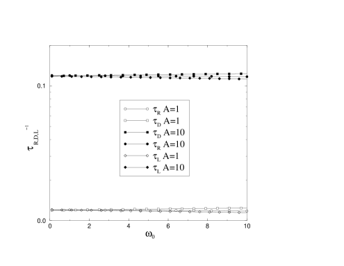
Figure 1: Dependence of the RDL rates on the spectral shifts for various spectral areas. Note that the vertical axis is logarithmic.

In Fig.(2) and for the same three level system the RDL rates are plotted against the spectral area for the rectangular spectrum. The curves obtained for the Lorentzian spectrum totally coincide with the corresponding ones for the rectangular spectrum and they are not shown. On the other hand, the same quantities are also plotted in Fig. (3) for the data obtained from the power-Gaussian spectrum for $\nu=-1,0,1$. The shown relaxation rates in Fig. (3) are indistinguishable from those in Fig. (2) within a very large range of spectral areas (The calculated dephasing and the leakage rates are in the same order of magnitude as the relaxation rates which can also be followed from Fig. (2); hence, they are not shown in the figure). These observations prove the independence from the shape of the spectrum. Moreover, the plots (a) for $\nu=1$, (b) for $\nu=0$ and (c) for $\nu=-1$ in Fig.(3) yield identical decoherence rates for the same horizontal scale. Hence, in the studied range $-1\leq\nu\leq 1$ corresponding to sub-Ohmic, Ohmic and super-Ohmic (i.e. $\nu=-1,0,1$ respectively) the decoherence rates are determined solely by the spectral area. This observation is contrary to the earlier beliefSB1 that it is the low frequency sector in the environmental spectrum [dominated by the $\omega^{1+\nu}$ term in (6)] dominating the RDL rates.

We hence observe independence from the shape and the type of spectrum within a large range of spectral areas covering three orders of magnitude. The log-log axes in Fig’s (2) and (3) additionally indicate that the RDL rates depend linearly on the spectral area. The monotonic dependence on the spectral area (whether it is a linear dependence or not), is a strong signature for the dominance of the non-resonant processes in the decoherence rates.

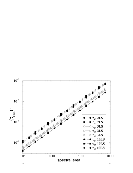
Figure 2: Dependence of the RDL rates on the spectral area for the spectral function (4). Note that the both axes are logarithmic. In generating the ten level results we assumed that the system’s energies above the first two levels are harmonic and given by $E_{n}=(n-1/2)~{},3\leq n$ and all the couplings are $\varphi_{n\,r}=0.1$ for $n+r=odd$ and zero otherwise.

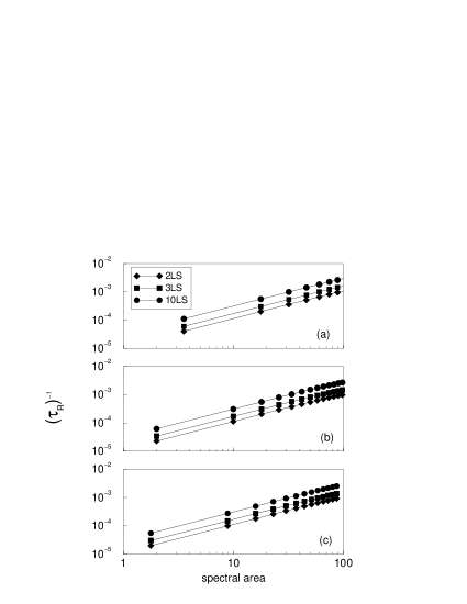
Figure 3: Dependence of the relaxation rates on the spectral area for the spectral function (6) corresponding to a) $\nu=1$ super-Ohmic, b) $\nu=0$ Ohmic, c) $\nu=-1$ sub-Ohmic spectra and for two, three and ten level systems. The trend for the dephasing and the leakage rates are very similar to Fig.(2) and they are not shown here. Note that the both axes are logarithmic. The energies $E_{n}$ and couplings $\varphi_{n\,r}$ of the multilevel system are as indicated in Fig.(2). The horizontal range in (c) is common to all graphs.

Additionally, in Fig.(2), and also implicitly in Fig.(3), the leakage rates are shown to be in the same order of magnitude as the RD rates. The leakage rates increase by the inclusion of higher levels [also see Fig.(4) in Section II.B below]. Hence, we conclude that, the leakage demonstrates itself to be a non-negligible short time effect manifested in multileveled systems.

The dominance of the non-resonant processes and their survival at zero temperature implies that the influence of the higher levels cannot be avoided independent from how well the qubit is energetically separated from those levels. This observation is in contrast with the assumption that, in low temperatures $T$ compared to the separation $\Delta E$ between the qubit subspace and higher states (i.e. $T\ll\Delta E$), the two level approximation is well satisfied.

II.2 The influence of the multilevels on RDL

The influence of the multilevels is examined by using a model coupling matrix $\varphi$ in (1) as

$$\varphi_{n\,r}=0.1\,e^{-|n-r|/\Delta}~{}$$ (7)

for $n+r=odd$ and zero otherwise. By varying the multilevel coupling range $\Delta$, the effect of the actively coupled levels on the RDL rates can be examined. In Fig.(4) the data is generated for different values of the multilevel range $\Delta=8,40$ and the spectral area $A=5,50$. The first observation is that, the linear trend observed in Fig.(2) against the spectral area is respected within a larger range of multilevels. Secondly, the multilevel coupling range is observed to give rise to a saturation in the RDL rates at the onset $M\simeq\Delta$. Fig.(4) therefore demonstrates further evidence of the observable effects in the decoherence rates arising from the finite coupling to multilevels.

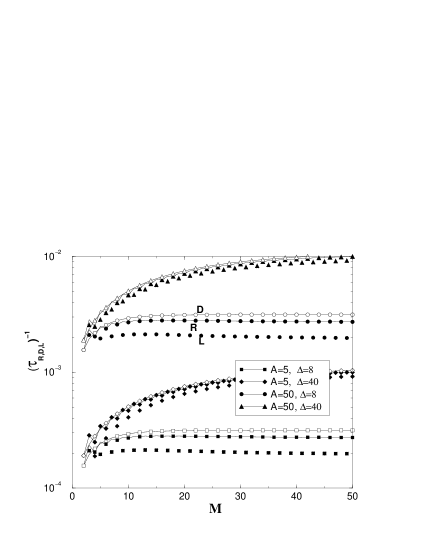
Figure 4: RDL rates at $T=0$ against the number of levels for different spectral areas and different multilevel coupling ranges $\Delta$. Here the coupling matrix elements between the levels $n$ and $r$ are modelled by $~{}\varphi_{n\,r}=0.1~{}e^{-|n-r|/\Delta}~{}~{}$ for $n+r=odd$ an zero otherwise. Note the logarithmic vertical axis. The open and solid symbols superimposed on the solid line refer to dephasing and relaxation rates respectively. The pure symbols without connecting lines refer to leakage rates. Also $(A,\Delta)$ values are $(5,8)$ for squares, $(5,40)$ for diamonds, $(50,8)$ for circles and $(50,40)$ for triangles. Here, the Lorentzian spectrum is used.

II.3 The fluctuations in the noise vacuum

A characteristic feature of the coordinate coupling is to produce weak vacuum fluctuations as well as finite number of environmental modes at zero temperature. These corrections, can be calculated perturbatively and they give a clue about the effectiveness of the virtual (non-resonant) processes.

The corrections to environmental number of modes can be calculated using the retarded Greens function

$$G_{\omega}(t-t^{\prime})=-i\Theta(t-t^{\prime})\,\langle{\cal T}\tilde{a}_{\omega}^{{\dagger}}(t)\tilde{a}_{\omega}(t^{\prime})\tilde{\cal S}(\infty,-\infty)\rangle$$ (8)

where ${\cal T}$ denotes the time ordering, the $~{}\tilde{}~{}$ denotes the interaction picture and the ${\cal S}$ matrix includes the interaction Hamiltonian in (1) in the interaction picture. The environmental photon number is than found by the standard method $n_{\omega}=i\lim_{t^{\prime}\to t}\,G_{\omega}(t-t^{\prime})$. The average is taken over the noninteracting initial state including system and the environment in the product form

$$|\rangle=(a|1\rangle+b|2\rangle)\otimes|env\rangle.$$ (9)

where $|env\rangle$ is characterized by the spectral function $I(\omega)$ at zero temperature. Evaluating the time ordered integrals arising from the expansion of the ${\cal S}$ matrix, and taking the limit $t^{\prime}\rightarrow t$ we obtain a second order correction as

$$\begin{array}[]{lrlr}{n}_{\omega}^{(2)}&&=\sum_{s=1}^{3}\frac{2I(\omega)}{\lambda_{s}^{2}}\\ &&\times(|a|^{2}\varphi_{0s}+|b|^{2}\varphi_{1s}+(a^{*}b+b^{*}a)\varphi_{1s}\varphi_{0s})\end{array}$$ (10)

where $\lambda_{s}=\omega+E_{1}-E_{s}$ and and $E_{1}=E_{2}$ as announced in (1). Eq.(10) yields a divergent result for the total number of photons even for arbitrarily small system-environment couplings. The divergence is obtained independently from the type of the spectrum in (4) or (5) and arises from the second order singularity in (10). To avoid this unphysical result in the second order, we convert the second order correction into an RPA sum following conventional practices in perturbative approachesMahan . As we use RPA, the second order pole in (10) is split into two first order poles which yields a finite result at the RPA level. The relevant RPA graphs are depicted in Fig. (5) below.

Figure 5: Contributing diagrams in the calculation of (11). (a) The definition of the basic second order root diagrams that are used to implement RPA. The dashed arc lines indicate the retarded limit $t^{\prime}\to t+0^{-}$ in the calculation of $n_{\omega}^{(2)}$, (b) the RPA hierarchy using the root diagram in (a), (c) the resulting RPA Green’s function used in the calculation of (12). Here the dashed arc lines indicate again the retarded limit $t^{\prime}\to t+0^{-}$ in the calculation of $n_{\omega}^{(RPA)}$.

Next, we calculate the fluctuations in the number of photons $\Delta n_{\omega}$ by using a four point retarded Green’s function for the environment as

$$D_{\omega}(t-t^{\prime})=-i\Theta(t-t^{\prime})\,\langle{\cal T}\tilde{a}_{k}^{{\dagger}}(t)\tilde{a}_{\omega}(t)\tilde{a}_{\omega}^{{\dagger}}(t^{\prime})\tilde{a}_{k}(t^{\prime})\tilde{\cal S}(\infty,-\infty)\rangle$$ (11)

The connected part of (11) directly yields the fluctuations in the photon number as $\Delta n^{2}_{\omega}=i\lim_{t^{\prime}\to t}\,D_{\omega}(t-t^{\prime})$. The diagrams corresponding to the RPA scheme using (11) are shown in Fig.(5). The fluctuation in the total photon number is found by $(\Delta N)^{2}=\int d\omega\,\Delta n^{2}_{\omega}$ and is given by

$$(\Delta N)^{2}=\sum_{s}\int_{-\infty}^{\infty}\frac{d\omega}{(\omega+\lambda_{s})}\frac{1}{1-4(system)_{s}I(\omega)/(\omega+\lambda_{s})}$$ (12)

which is plotted in Fig.(6) with respect to $\epsilon$ and parameterized by $\omega_{0}$ for the two, three and ten level systems. The bare spectral area is fixed at $A=5\pi$. The observed independence from $\epsilon$ at fixed spectral area implies independence from the spectral shape. Additionally independence from $\omega_{0}$ is also shown.

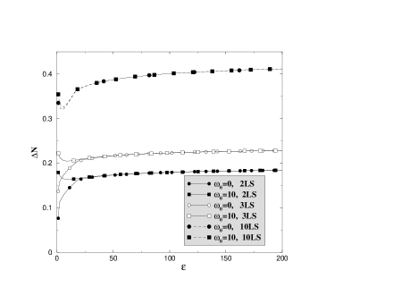
Figure 6: Fluctuations in the total photon number versus the spectral width for various $\omega_{0}$ values computed for two three and ten leveled MLS. Here the bare spectral area $A=5\pi$

In Fig.(7) below, the ratio $\Delta N/N$ is plotted as a function of the spectral area. The figure, together with the inlet for $\Delta N$ versus spectral area, is well fitted to

$$\frac{\Delta N}{N}\simeq\frac{Const.}{\sqrt{A}}$$ (13)

We observe that $\Delta N\propto\sqrt{A}$ and $N\propto A$ in a large range of spectral areas. Here the positive constant $Const.$ depends on the number of multi levels.

Figure 7: The ratio $\Delta N/N$ versus the spectral area (inlet: $\Delta N$ versus the spectral area).

The results of this subsection are in a sense also a check for the validity of the Born-Oppenheimer approximation. The correction obtained to the spectral area as a result of the system-environment coupling is bounded by a few ten percent. However, as the number of levels increase the total fluctuations decrease relative to the increase in the total number of environmental modes. For a MLS with strong couplings between a large number of levels the validity of the Born-Oppenheimer approximation may still survive although we did not check this result explicitly.

III Conclusions

It is shown that for the most conventionally used system-environment couplings of linear coordinate type the non-resonant processes overwhelm the resonant ones in their contribution to the decoherence rates at zero temperature. In this regard, and within the studied spectral range, it is observed that the decoherence rates do not depend on the specific low/high energy properties of the spectrum, whereas, a strong (and dominantly) dependence is observed on the overall spectral area. These results are confirmed for three independent spectral profiles.

We have also examined the effect of the system-environment coupling. We observed that the number of levels which are coupled by the system-environment coupling plays a non-negligible role in decoherence time rates. We see that as the number of coupled levels in the system increase, both the decoherence time rates and photon number corrections increase further from the rates and corrections in a pure two level system. The observed effects for the MLS cannot be explained by an equivalent renormalization of the two levelled subsystem. In the light of these observations, we conclude that the conventional postulates of the two-level approximation do not necessarily lead to a dynamical behaviour of a multilevelled system largely confined to its lowest two levels. The presented results are obtained from the numerical solution of the master equation with the Born-Oppenheimer approximation, and hence, they are exact in the short time limit where the decoherence properties are studied.

IV Acknowledgements

This research is supported by the Scientific and the Technical Research Council of Turkey (TÜBİTAK) grant number TBAG-2111 (101T136) and by the Dicle University grant number DÜAPK-02-FF-27. E. Meṣe thanks the Bilkent University for hospitality. We thank C. Sevik for his help with the Fig.(5).

References

- (1) A.O. Caldeira and A.J. Leggett, Phys. Rev. Lett. 46, 211 (1981); A.O. Caldeira and A.J. Leggett, Annals of Physics 149, 374 (1983).
- (2) A.J. Leggett and Anupam Garg, Phys. Rev. Lett. , 54, 857 (1985).
- (3) T. Hakioğlu and Kerim Savran, Role of the environmental spectrum in the decoherence and dephasing of multilevel quantum systems, Phys. Rev. B, to appear.
- (4) Guido Burkard, Roger H. Koch and David P. Di Vincenzo, Phys. Rev. B 69, 064503 (2004).
- (5) A.J. Leggett, S. Chakravarty, A.T. Dorsey, Matthew P.A. Fisher, Anupam Garg and W. Zwerger, Rev. Mod. Phys. 59, 1 (1987); Daniel Loss andDavid P DiVincenzo, Exact Born Approximation for the spin-boson model, [cond-mat/0304118]; Till Vorrath, Tobias Brandes Bernhard Kramer, Dynamics of a large spin-boson system in the strong coupling regime, [cond-mat/0111220]; M. Grifoni, E. Paladino and U. Weiss, Eur. Phys. J B 10, 719 (1999).
- (6) Charis Anastopoulos and B.L. Hu, Phys. Rev. A62, 033821 (2000).
- (7) M. Dube and P.C.E. Stamp, Mechanism of Decoherence at low Temperatures, Chem. Phys. Quantum Physics of Open Systems, Special Issue (2001) also [cond-mat/0102156]; P.C.E. Stamp, I.S. Tupitsyn, Chem. Phys. 296 281 (2004); Leonid Fedichkin, Akrady Fedorov and Vladimir Privman, Proc. SPIE 5105, 243 (2003).
- (8) D. Natelson, R. L. Willett, K. W. West, and L.N. Pfeiffer Phys. Rev. Lett. 86, 1821 (2001).
- (9) Pascal Cedraschi, Vadim V. Ponomarenko and Markus Büttiker, Phys. Rev. Lett. 84, 346 (2000); M. Büttiker, EDP Sciences, 231 (2001).
- (10) J.J. Lin and N. Giordano, Phys. Rev. B 35, 1071 (1987); D.M. Pookr t al. J. Phys. Cond. Matt. 1, 3289 (1989).
- (11) P. Mohanty, E.M.Q. Jariwala and R.A. Webb, Phys. Rev. Lett. 78, 3366 (1997); P. Mohanty and R.A. Webb, Phys. Rev. B 55, R13452 (1997).
- (12) M. Born and J.R. Oppenheimer, Ann. Phys. 84, 457 (1927); Arno Bohm and Mark Loewe, Quantum Mechanics, Springer Verlag 2001.
- (13) Gerald Mahan, Many Particle Physics, Plenum Press 1990.
- (14) Guido Burkard, Roger H. Koch and David P. DiVincenzo, Phys. Rev. B 69, 064503 (2004).