Quantum state transmission via a spin ladder as a robust data bus

Abstract

We explore the physical mechanism to coherently transfer the quantum information of spin by connecting two spins to an isotropic antiferromagnetic spin ladder system as data bus. Due to a large spin gap existing in such a perfect medium, the effective Hamiltonian of the two connected spins can be archived as that of Heisenberg type, which possesses a ground state with maximal entanglement. We show that the effective coupling strength is inversely proportional to the distance of the two spins and thus the quantum information can be transferred between the two spins separated by a longer distance, i.e. the characteristic time of quantum state transferring linearly depends on the distance.

Transferring a quantum state from a quantum bit to another is not only the central task in the quantum communication, but also is often required in scalable quantum computing based on the quantum network q-inf . In the latter, one should connect different quantum predeceasing units in different locations with a medium called data bus. The typical examples of quantum state transfer is the quantum storage based on various physical systemsHau ; Lukin , such as the quasi-spin wave excitations s-prl . For the solid state based quantum computing at the large-scale, it is very crucial to have a solid system serving as such quantum data bus, which can provide us with a quantum channel for quantum communication q-solid . Most recently the simple spin chain, a typical solid state system, is considered as a coherent data bus Bose ; Subra ; Matt . The quantum transmission of state is achieved by placing two spins at the two ends of the chain. These schemes may admit an efficient state transfer of any quantum state in a fixed period of time of the state evolution, but the crucial problem is the dependence of transferring efficiency on communication distance. In usual the efficiency is inversely proportional to square or higher order power of the distance of the two spins and thus such quantum state transmission can only works efficiently in a much shorter distance.

The aim of this letter is to solve this short-distant transfer problem by replacing the simple spin chain with an isotropic antiferromagnetic spin ladder. Because the this kind of spin ladder possesses a finite spin gap, an effective Heisenberg interaction can be induced in the stable ground state channel to achieve the maximally entangled states that implement a more fast quantum states transfer of two spin qubits attached to this spin ladder system. Actually, when the spin gap is sufficiently large comparing to the coupling strength between two spin qubits and the spin ladder, the perturbation method can be performed. Analytical and numerical results show that the spin ladder system is a perfect medium through which the interaction between two distant spins can be mapped to an approximate Heisenberg type coupling with a coupling constant inversely proportional to the distance between the two separated spins.

It is well known that there are two ways to transfer quantum information: one can first use the channel to share entanglement with separated Alice and Bob and then use this entanglement for teleportationQtele , or directly transmit a state through a quantum data bus. For the latter it seems that the long distance entanglement is not necessary to interface different kinds of physical systems, but and it will be showed in this letter that there hides an effective entanglement intrinsically. In this senses a quantum state transmission can be generally understood through such quantum entanglement.

We sketch our idea with the model illustrated in Fig.1 The whole quantum system we consider here consists of two qubits (A and B) and a $2\times N$-site two-leg spin ladder. In practice, this system can be realized by the engineered array of quantum dots QD array . The total Hamiltonian

$$H=H_{M}+H_{q}$$ (1)

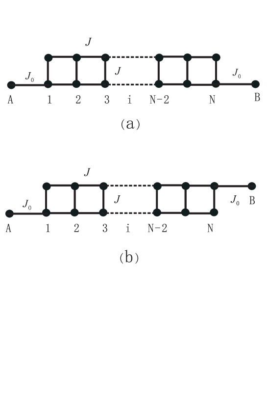
Figure 1: Two qubits $A$ and $B$ connect to a $2\times N$-site spin ladder. The ground state of $H$ with a-type connection (Fig.1(a)) is singlet (triplet) when $N$ is even (odd), while for b-type connection (Fig.1(b)), one should have opposite result.

contains two parts, the medium Hamiltonian

$$H_{M}=J\sum_{\left\langle ij\right\rangle\perp}\overrightarrow{S}_{i}\cdot\overrightarrow{S}_{j}+J\sum_{\left\langle ij\right\rangle\parallel}\overrightarrow{S}_{i}\cdot\overrightarrow{S}_{j}$$ (2)

describing the spin-1/2 Heisenberg spin ladder consisting of two coupled chains and the coupling Hamiltonian

$$H_{q}=J_{0}\overrightarrow{S}_{A}\cdot\overrightarrow{S}_{L}+J_{0}\overrightarrow{S}_{B}\cdot\overrightarrow{S}_{R}$$ (3)

describing the connections between qubits $A$, $B$ and the ladder. In the term $H_{M},$ $i$ denotes a lattice site on which one electron sits, $\left\langle ij\right\rangle$ $\perp$ denotes nearest neighbor sites on the same rung, $\left\langle ij\right\rangle$ $\parallel$ denotes nearest neighbors on either leg of the ladder. In term $H_{q}$, $L$ and $R$ denote the sites connecting to the qubits $A$ and $B$ at the ends of the ladder. There are two types of the connection between $\overrightarrow{S}_{A}(\overrightarrow{S}_{B})$ and the ladder, which are illustrated in Fig.1. According to the Lieb’s theorem Lieb , the spin of the ground state of $H$ with the connection of type a is zero (one) when $N$ is even (odd), while for the connection of type b, one should have an opposite result. For the two-leg spin ladder $H_{M},$ analytical analysis and numerical results have shown that the ground state and the first excited state of the spin ladder have spin $0$ and $1$ respectively Dagotto ; White . It is also shown that there exists a finite spin gap

$$\triangle=E_{1}^{M}-E_{g}^{M}\sim J/2.$$ (4)

between the ground state and the first excited state (see the Fig.2). This fact has been verified by experiments Dagotto and is very crucial for our present investigation.

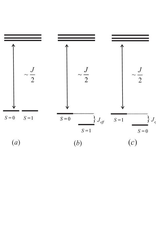
Figure 2: Schematic illustration of the energy levels of the system. (a) When the connections between two qubits and the medium switch off ($J_{0}=0$) the ground states are degenerate. (b), (c) When $J_{0}$ switches on, the ground state(s) and the first excited state(s) are either singlet or triplet. This is approximately equivalent to that of two coupled spins.

Thus, it can be concluded that the medium can be robustly frozen its ground state to induced the effective Hamiltonian

$$H_{eff}=J_{eff}\overrightarrow{S}_{A}\cdot\overrightarrow{S}_{B}$$ (5)

between the two end qubits. With the effective coupling constant $J_{eff}$ to be calculated in the following, this Hamiltonian depicts the direct exchange coupling between two separated qubits. As the famous Bell states, $H_{eff}$ has singlets and triplets eigenstates $\left|j,m\right\rangle_{AB}:$ $\left|0,0\right\rangle=$ $\frac{1}{\sqrt{2}}\left(\left|\uparrow\right\rangle_{A}\left|\downarrow\right\rangle_{B}-\left|\downarrow\right\rangle_{A}\left|\uparrow\right\rangle_{B}\right)$ and $\left|1,1\right\rangle=\left|\uparrow\right\rangle_{A}\left|\uparrow\right\rangle_{B}$ ,$\left|1,-1\right\rangle=\left|\downarrow\right\rangle_{A}\left|\downarrow\right\rangle_{B},\left|1,0\right\rangle$ $=\frac{1}{\sqrt{2}}\left(\left|\uparrow\right\rangle_{A}\left|\downarrow\right\rangle_{B}+\left|\downarrow\right\rangle_{A}\left|\uparrow\right\rangle_{B}\right),$which can be used as the channel to share entanglement for a perfect quantum communication in a longer distance.

The above central conclusion can be proved both with the analytical  and numerical methods as follows. To deduce the above effective Hamiltonian we utilize the Frőhlich transformation, whose original approach was used successfully for the superconductivity BCS theory. As a second order perturbation, the effective Hamiltonian $H_{\mathrm{eff}}\cong H_{\mathrm{M}}+\frac{1}{2}\left[H_{\mathrm{q}},S\right]$ can be achieved approximately by a unitary operator $U=\exp\{-S\}$ where anti-Hermitian operator $S$, obeys $H_{\mathrm{q}}+[H_{\mathrm{M}},S]=0.$Let $\left|m\right\rangle$ and $E_{m}$ are the eigenvectors and eigenvalues of $H_{M}=$ $H(J_{0}=0)$ respectively.

From the explicit expressions for the elements $S_{mn}$ = $\left(H_{\mathrm{q}}\right)_{\mathrm{mn}}/(E_{\mathrm{m}}-E_{\mathrm{n}}),(m\neq n),S_{mm}=0$, the matrix elements of effective Hamiltonian can be achieved approximately as

$$\left\langle n\right|H_{\mathrm{eff}}\left|m\right\rangle\cong E_{\mathrm{m}}\delta_{mn}+\underset{\mathrm{k}\neq\mathrm{m}}{\sum}\frac{\left(H_{\mathrm{q}}\right)_{\mathrm{nk}}\left(H_{\mathrm{q}}\right)_{\mathrm{km}}}{2(E_{\mathrm{k}}-E_{\mathrm{m}})}-\underset{\mathrm{k}\neq\mathrm{n}}{\sum}\frac{\left(H_{\mathrm{q}}\right)_{\mathrm{nk}}\left(H_{\mathrm{q}}\right)_{\mathrm{km}}}{2(E_{\mathrm{n}}-E_{\mathrm{k}})}.$$ (6)

We use $|\psi_{g}\rangle_{M}$ ($|\psi_{\alpha}\rangle_{M}$) and $E_{g}$ ($E_{\alpha}$) to denote ground (excited) states of $H_{\mathrm{M}}$ and the corresponding eigen-values. The zero order eigenstates $\left|m\right\rangle$ can then be written as in a joint way

$$\left|j,m\right\rangle_{g}=\left|j,m\right\rangle_{AB}\otimes|\psi_{g}\rangle_{M},\left|\psi_{\alpha}^{jm}(s^{z})\right\rangle=\left|j,m\right\rangle_{AB}\otimes|\psi_{\alpha}\rangle_{M}$$ (7)

Here, we have considered that z-component $S^{z}=S_{M}^{z}+S_{A}^{z}+S_{B}^{z}$ of total spin  is conserved with respect to the connection Hamiltonian $H_{q}$. Since $S_{M}^{z}$ and $S_{M}^{2}$ conserves with respect to $H_{M}$ we can label $|\psi_{g}\rangle_{M}$ as $|\psi_{g}(s_{M},s_{M}^{z},)\rangle_{M}$ and then $s^{z}=m+s_{M}^{z}$ can characterize the non-coupling spin state $\left|\psi_{\alpha}^{jm}(s^{z})\right\rangle.$

When the connections between two qubits and the medium switch off, i.e., $J_{0}=0,$ the degenerate ground states of $H$ are just $\left|j,m\right\rangle_{g}$ with the degenerate energy $E_{g}$ and spin $0,1$ respectively, which is illustrated in Fig.2 (a). When the connections between the two qubits and the medium switch on, the degenerate states with spin $0,1$ should split as illustrated in Fig.2 (b) and (c). In the case with $J_{0}\ll J$ at lower temperature $kT<J/2$ , the medium can be frozen in its ground state and then we have the effective Hamiltonian

$$H_{\mathrm{eff}} \cong \sum_{j^{\prime},m^{\prime},j,m,s^{z}}\frac{|_{g}\left\langle j,m\right|H_{\mathrm{q}}\left|\psi_{\alpha}^{j^{\prime}m^{\prime}}(s^{z})\right\rangle|^{2}}{E_{g}-E_{\mathrm{\alpha}}}\left|j,m\right\rangle_{gg}\left\langle j,m\right|$$

$$= J_{eff}.\mathit{Diag}.(\frac{1}{4},\frac{1}{4},\frac{1}{4},-\frac{3}{4})+\varepsilon$$

where

$$J_{eff} = \sum\limits_{\alpha}\frac{J_{0}^{2}[L(\alpha)R^{\ast}(\alpha)+R(\alpha)L^{\ast}(\alpha)]}{E_{g}-E_{\alpha}},$$ (7)

$$\varepsilon = \sum\limits_{\alpha}\frac{3J_{0}^{2}\left[\left|L(\alpha)\right|^{2}+\left|R(\alpha)\right|^{2}\right]}{4\left(E_{g}-E_{\alpha}\right)}.$$

This just proves the above effective Heisenberg Hamiltonian (5). Here, the matrix elements of interaction $K(\alpha)=_{M}\left\langle\psi_{g}\right|S_{K}^{z}\left|\psi_{\alpha}\left(1,0\right)\right\rangle_{M}$ ($K=S,L)$ can be calculated only for the variables of data bus medium. We also remark that, because $S^{z}$ and $S^{2}$ are conserved for $H_{q},$ off-diagonal elements in the above effective Hamiltonian vanish.

In temporal summary, we have shown that at lower temperature $kT<J/2,$ $H$ can be mapped to the effective Hamiltonian (5), which semmingly depicts the direct exchange coupling between two separated qubits. Notice that the coupling strength has the form $J_{eff}\sim g(L)J_{0}^{2}/J,$, where $g(L)$ is a function of $L=N+1$, the distance between the two qubits we concerned. Here we take the $N=2$ case as an example. According to Eq.(9) one can get $J_{eff}=-\frac{1}{4}J_{0}^{2}/J$ and $\frac{1}{3}J_{0}^{2}/J$ when $A$ and $B$ connect the plaquette diagonally and adjacently, respectively. This result is in agreement to the theorem Lieb about the ground state and the numerical result when $J_{0}\gg J$. In general case, the behavior $g(L)$ vs $L$ is very crucial for quantum information since $L/\left|J_{eff}\right|$ determines the characteristic time of quantum state transfer between the two qubits $A$ and $B$. In order to investigate the profile of $g(L),$ a numerical calculation is performed for the systems $L=4,5,6,7,8,$ and $10$, with $J=10,20,40,$ and $J_{0}=1$. The spin gap between the ground state(s) and first excite state(s) are calculated, which corresponds to the magnitude of $J_{eff}$. The numerical result is plotted in Fig.3 , which indicates that $J_{eff}\sim 1/(LJ)$. It implies that the characteristic time of quantum state transfer linearly depends on the distance and then guarantees the possibility to realize the entanglement of two separated qubits in practice.

In order to verify the validity of the effective Hamiltonian $H_{eff}$, we need to compare the the eigen states of $H_{eff}$ with those reduced states from the eigen states of total system. In general the eigenstates of $H$ can be written formally as

$$\left|\psi\right\rangle=\sum_{jm}c_{jm}\left|j,m\right\rangle_{AB}\otimes|\beta_{jm}\rangle_{M}$$ (8)

where {$|\beta_{jm}\rangle_{M}$ } is a set of vectors of the data bus, which is not necessarily orthogonal. Then we have the condition $\sum_{jm}|c_{jm}|_{M}^{2}\langle\beta_{jm}|\beta_{jm}\rangle_{M}=1$for normalization of $\left|\psi\right\rangle$. In this sense the practical description of the A-B subsystem of two quits can be only given by the reduced density matrix

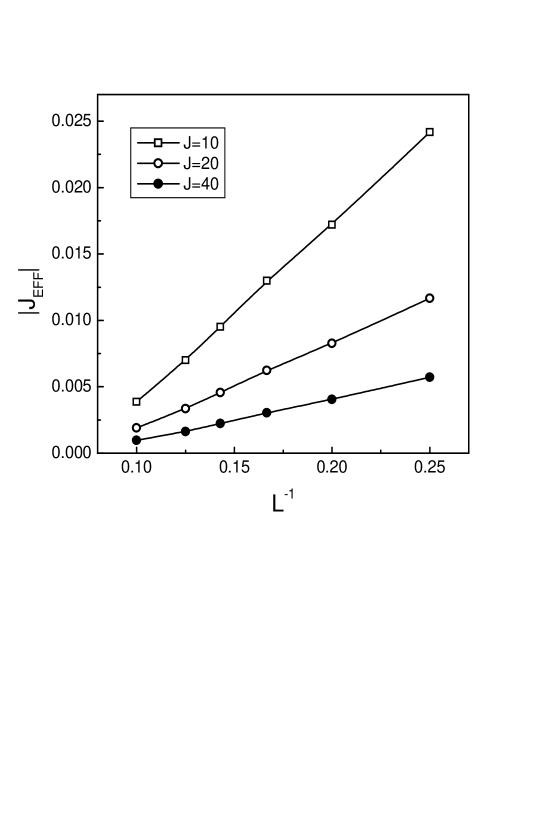
Figure 3: The spin gaps obtained by numerical method for the systems $L=4,5,6,7,8,$ and $10$, with $J=10,20,40,$ and $J_{0}=1$ are potted, which is corresponding to the magnitude of $J_{eff}$. It indicates that $J_{eff}\sim 1/(LJ)$.

$$\rho_{AB} = Tr_{M}(\left|\psi\right\rangle\left\langle\psi\right|)=\sum_{jm}|c_{jm}|^{2}\left|j,m\right\rangle_{AB}\langle j,m|$$

$$+\sum_{j^{\prime}m^{\prime}\neq jm}c_{j^{\prime}m^{\prime}}^{\ast}c_{jmM}\langle\beta_{j^{\prime}m^{\prime}}|\beta_{jm}\rangle_{M}\left|j,m\right\rangle_{AB}\langle j^{\prime},m^{\prime}|$$

where $Tr_{M}$ means the trace over the variables of the medium. By a straightforward calculation we have

$$\left|c_{11}\right|^{2} = \left|c_{1-1}\right|^{2}=\left\langle\psi\right|\left(\frac{1}{4}+S_{A}^{z}\cdot S_{B}^{z}\right)\left|\psi\right\rangle,$$

$$\left|c_{00}\right|^{2} = \left\langle\psi\right|\left(\frac{1}{4}-\overrightarrow{S}_{A}\cdot\overrightarrow{S}_{B}\right)\left|\psi\right\rangle,$$ (10)

$$\left|c_{10}\right|^{2} = 1-2\left|c_{11}\right|^{2}-\left|c_{00}\right|^{2}.$$

Now we need a criteria to judge how close the practical reduced eigenstate by the above reduced density matrix (11) to the pure state for the effective two sites coupling $H_{eff}$. As we noticed, it has the singlet and triplet eigenstates $\left|j,m\right\rangle_{AB}$ in the subspace spanned by $\left|0,0\right\rangle_{AB}$ with $S^{z}=S_{A}^{z}+S_{B}^{z}=0$, we have $\left|c_{11}\right|^{2}=\left|c_{10}\right|^{2}=\left|c_{1-1}\right|^{2}=0,$ $\left|c_{00}\right|^{2}=1;$ for triplet eigen state $\left|1,0\right\rangle_{AB}$, we have $\left|c_{11}\right|^{2}=\left|c_{1-1}\right|^{2}=\left|c_{00}\right|^{2}=0,$ $\left|c_{10}\right|^{2}=1$. With the practical Hamiltonian $H,$ the values of $\left|c_{jm}\right|^{2},\quad i=1,2,3,4$ are numerically calculated for the ground state $\left|\psi_{g}\right\rangle$ and first excited state $\left|\psi_{1}\right\rangle$ of finite system systems $L=4,5,6,7,8$ and $10$ with $J=10,20,$ and $40,$ $(J_{0}=1)$ in $S^{z}=0$ subspace, which are listed in the Table 1(a,b,c). It shows that, at lower temperature, the realistic interaction leads to the results about $\left|c_{jm}\right|^{2}$, which are very close to that described by $H_{eff},$ even if $J$ is not so large in comparison with $J_{0}.$

Table 1. The diagonal elements of reduced density matrix, which provide a criteria for the validity of $H_{eff},$, are calculated numerically for the ground state and first excited state of finite system systems $L=4,5,6,7,8$ and $10.$ The results for $J=10,20,$ and $40,(J_{0}=1)$ are listed in (a), (b), and (c) respectively. It shows that, at lower temperature, the result based the realistic interaction is very close to that by $H_{eff}.$

We remark that the above tables reflect all the facts distinguishing the difference between the results about the entanglement of two end qubit generated by $H_{eff}$ and $H.$ Though we have ignored the considerations for the off-diagonal terms in the reduced density matrix, the calculation of the feudality $F(|j,m\rangle)\equiv._{M}\langle j,m|\rho_{AB}|j,m\rangle_{M}=|c_{jm}|^{2}$ further confirm our observation that, the effective Heisenberg type interaction of two end qubits can approximates the realistic Hamiltonian very well. Then we can transfer the quantum information between two ends of the $2\times N$-site two-leg spin ladder that can be regarded as the channel to share entanglement with separated Alice and Bob. Physically, this is just due to a large spin gap existing in such a perfect medium, whose ground state can induce a maximal entanglement of the two end qubits. We also pointed out that our analysis is applicable for other types of medium systems as data buses, which possess a finite spin gap. Since $L/\left|J_{eff}\right|$ determines the characteristic time of quantum state transfer between the two qubits, the dependence of $J_{eff}$ upon $L$ becomes important and relies on the appropriate choice of the medium.

In conclusion, we have presented and studied in details a protocol to achieve the entangled states and fast quantum states transfer of two spin qubits by connecting two spins to a medium which possesses a spin gap. A perturbation method, the Frőhlich transformation, shows that the interaction between the two spins can be mapped to the Heisenberg type coupling. Numerical results show that the isotropic antiferromagnetic spin ladder system is a perfect medium through which the interaction between two separated spins is very close to the Heisenberg type coupling with a coupling constant inversely proportional to the distance even if the spin gap is not so large comparing to the couplings between the input and output spins with the medium.

This work of SZ is supported by the Cooperation Foundation of Nankai and Tianjin university for research of nanoscience. CPS also acknowledge the support of the CNSF (grant No. 90203018) , the Knowledge Innovation Program (KIP) of the Chinese Academy of Sciences, the National Fundamental Research Program of China (No. 001GB309310).

References

- (1) D. Bouwmeeste, A. Ekert, and A. Zeilinger (Ed.), The Physics of Quantum Information (Springer, Berlin, 2000).
- (2) C. Liu, Z. Dutton, C. H. Behroozi, and L. V. Hau, Nature 409, 490 (2001).
- (3) M. D. Lukin, Rev. Mod. Phys. 75, 457 (2003).
- (4) C. P. Sun, Y. Li, and X. F. Liu, Phys. Rev. Lett. 91, 147903 (2003).
- (5) D. P. DiVincenzo and C. Bennet, Nature 404, 247 (2000) and references therein
- (6) S. Bose, Phys. Rev. Lett. 91, 207901 (2003).
- (7) V. Subrahmanyam, Phys. Rev. A69, 034304 (2004).
- (8) M. Christandl, N. Datta, and J. Landahl, Phys. Rev. Lett. 92, 187902 (2004).
- (9) C.H. Bennett, G. Brassard, C. Crepeau, R. Jozsa, A. Peres, and W. Wootters, Phys. Rev. Lett. 70, 895 (1993)
- (10) D. Loss and D. P. DiVincenzo, Phys. Rev. A 57, 120 (1998); B. E. Kane, Nature (London) 393, 133 (1998).
- (11) E. Dagotto and T. M. Rice, Science 271, 618 (1996).
- (12) S. White, R. Noack, and D. Scalapino, Phys. Rev. Lett. 73, 886 (1994); R. Noack, S. White, and D. Scalapino, Phys. Rev. Lett. 73, 882 (19940).
- (13) E. Lieb, Phys. Rev. Lett. 62, 1201 (1989); E. Lieb and D. Mattis, J. Math. Phys. 3, 749 (1962).
- (14) Z. Song, Phys. Lett. A 231, 135 (1997); Z. Song, Phys. Lett. A 233, 135 (1997).