Vacuum fluctuations and the conditional homodyne detection of squeezed light

Abstract

Conditional homodyne detection of quadrature squeezing is compared with standard nonconditional detection. Whereas the latter identifies nonclassicality in a quantitative way, as a reduction of the noise power below the shot noise level, conditional detection makes a qualitative distinction between vacuum state squeezing and squeezed classical noise. Implications of this comparison for the realistic interpretation of vacuum fluctuations (stochastic electrodynamics) are discussed.

1 Introduction

The field of quadrature squeezing saw its main period of growth in the 1980’s [1, 2, 3]. The topic continues to be important to many areas of research involving nonclassical light and its applications [4, 5, 6, 7]. In this paper we discuss one of the earliest and most fundamental issues addressed in this field: the detection of quadrature squeezed light and the characterization of squeezing as a nonclassical effect.

The standard squeezing measurement uses balanced homodyne detection [8]. In this scheme, nonclassical squeezing is identified with a reduction of the measured noise variance below the shot noise level. The noise variance depends on the phase of the local oscillator, in such a way that the reduction evolves into an enhancement as the phase is continuously changed. In this standard measurement the shot noise level is the “measuring stick”, used to differentiate quantum from classical squeezing in a quantitative way. Considered for the qualitative response only, the two types of squeezing appear in the same way. In either case, one observes a phase-sensitive reduction of the noise variance over a limited bandwidth; as stated, the distinction made is purely quantitative: a reduction below the shot noise level is a quantum effect, otherwise the squeezing is classical.

There is nothing particularly curious in this. Other instances exist in quantum optics where nonclassicality is defined by the violation of a quantitative bound; one might prefer that the bound be a relative measure—a fringe visibility, for example; on the other hand, there is no reason to doubt that the shot noise level can be reliably set.

At a more fundamental level, however, it does seem reasonable to expect that the difference between quantum and classical noise would amount to something more than the mere size of a noise variance. If, after all, that is the only distinction, the natural conclusion is that quantum and classical fluctuations are qualitatively the same. Classical noise models, such as stochastic electrodynamics, should then be adequate to account for quantum noise.

We show in this paper that in the case of quadrature squeezing the expected qualitative difference does exist. It is revealed by a measurement based on conditional homodyne detection [9, 10]. Our proposal is not the first to make a qualitative distinction between classical and quantum squeezing, since such differences also appear in the response of atoms illuminated by squeezed light [11]. In contrast to this earlier work, however, our proposal makes the distinction at the level of an elementary squeezing measurement.

In section 2 we review the theoretical treatment of quadrature squeezing of broadband classical noise and its extension to the quantum case via the Wigner representation. Section 3 discusses the detection of squeezed light, and contrasts nonconditional and conditional homodyne detection schemes. The implications of the demonstrated qualitative difference between quantum and classical squeezing for the realistic interpretation of vacuum fluctuations (stochastic electrodynamics) is discussed in section 4. Brief conclusions are then drawn in section 5.

2 Quadrature squeezing as a property of the electromagnetic field

Quadrature squeezing is commonly understood as a property of the electromagnetic field, without referring to how that property will be measured. This way of thinking is certainly unproblematic so far as squeezed classical noise is concerned. We therefore begin from this point of view and review the well-known results for the quadrature squeezing of a broadband classical noise field, ${\cal E}_{\rm in}(z,t)$ in figure 1, injected into the input of a below-threshold degenerate parametric oscillator (DPO). The squeezing observed at the output is readily understood by considering how ${\cal E}_{\rm out}(z,t)$ is formed from the interference of ${\cal E}_{\rm in}(z,t)$ with the partial transmission, through the output mirror, of the intracavity field $\alpha(t)$ [12]. The spectrum of the squeezing may be calculated in the following straightforward way.

Figure 1: Sketch of the ring-cavity DPO squeezer with single input-output port. The shaded region represents the $\chi^{(2)}$ nonlinear crystal.

2.1 Squeezed classical noise

We first expand the input and output fields in terms of traveling-wave modes satisfying periodic boundary conditions on an interval of length $2L$ (figure 1). Mode frequencies are denoted by $\omega+\omega_{0}$, where $\omega_{0}$ is the resonance frequency of the DPO cavity. The fields, in photon flux units, are then given by

$${\cal E}_{\rm in}(z,t) = \sum_{\omega}\sqrt{c/2L}\mkern 2.0muf_{\omega}\exp[-\rmi(\omega_{0}+\omega)(t-z/c)],$$ (2.1)

$${\cal E}_{\rm out}(z,t) = \sum_{\omega}\left(\mkern-2.0mu\sqrt{c/2L}\mkern 2.0muf_{\omega}+\sqrt{2\kappa}\mkern 2.0mu\alpha_{\omega}\right)\exp[-\rmi(\omega_{0}+\omega)(t-z/c)],$$ (2.2)

where the complex amplitudes $f_{\omega}$ are random variables, of zero mean, and with covariances

$$\overline{f_{\omega}f_{\omega^{\prime}}}=\overline{f_{\omega}^{*}f_{\omega^{\prime}}^{*}}=0,\qquad\overline{f_{\omega}^{*}f_{\omega^{\prime}}}=\bar{n}\delta_{\omega\omega^{\prime}};$$ (2.3)

the input-field noise spectrum is thus assumed to be flat with an average strength of $\bar{n}$ photons per mode. The intracavity field is expanded in a similar way as

$$\alpha(t)=\sum_{\omega}\alpha_{\omega}\rme^{-\rmi(\omega_{0}+\omega)t},$$ (2.4)

and the advertised interference of ${\cal E}_{\rm in}(z,t)$ with $\alpha(t)$ appears explicitly as a sum of amplitudes $f_{\omega}$ and $\alpha_{\omega}$ on the right-hand side of equation (2.2). We also introduce the two-mode quadrature amplitudes [13, 14]

$$\eqalign{X_{\omega}&\equiv(f_{\omega}+f_{-\omega}^{*})/2,\cr\vskip 2.0pt\cr Y_{\omega}&\equiv-\rmi(f_{\omega}-f_{-\omega}^{*})/2,}\qquad\eqalign{x_{\omega}&\equiv(\alpha_{\omega}+\alpha_{-\omega}^{*})/2,\cr\vskip 2.0pt\cr y_{\omega}&\equiv-\rmi(\alpha_{\omega}-\alpha_{-\omega}^{*})/2.}$$ (2.9)

Note that these are complex quadrature amplitudes and correspond to non-Hermitian quantum operators (except when $\omega=0$).

The root cause of squeezing is the phase-sensitive amplification and deamplification of the intracavity field. It arises because the amplitude $\alpha_{\omega}$ couples to $\alpha_{-\omega}^{*}$ through the $\chi^{(2)}$ nonlinearity of the intracavity crystal. In addition, $\alpha_{\omega}$ is excited by $f_{\omega}$ and damped at the rate $\kappa$. The pair of coupled amplitude equations are

$$0 = -(\kappa-\rmi\omega)\alpha_{\omega}+\kappa\lambda\alpha_{-\omega}^{*}-\sqrt{c/2L}\sqrt{2\kappa}\mkern 2.0muf_{\omega},$$ (2.10)

$$0 = -(\kappa-\rmi\omega)\alpha_{-\omega}^{*}+\kappa\lambda\alpha_{\omega}-\sqrt{c/2L}\sqrt{2\kappa}\mkern 2.0muf_{-\omega}^{*},$$ (2.11)

where $\lambda$ is a (real) parameter proportional to $\chi^{(2)}$ and the amplitude of the field that pumps the nonlinear crystal; the threshold for sustained oscillation of the DPO occurs at $\lambda=1$. The solution of equations (2.10) and (2.11) for the frequency-dependent intracavity quadrature amplitudes is

$$x_{\omega} = -\sqrt{\frac{c}{2L}}\sqrt{2\kappa}\mkern 2.0mu\frac{X_{\omega}}{\kappa(1-\lambda)-\rmi\omega},$$ (2.12)

$$y_{\omega} = -\sqrt{\frac{c}{2L}}\sqrt{2\kappa}\mkern 2.0mu\frac{Y_{\omega}}{\kappa(1+\lambda)-\rmi\omega},$$ (2.13)

which when substituted into equation (2.2) yield the relationship between output- and input-field quadrature amplitudes. The spectra of squeezing are thus given by the intensities

$$\frac{2L}{c}\overline{\left|\sqrt{c/2L}\mkern 2.0muX_{\omega}+\sqrt{2\kappa}\mkern 2.0mux_{\omega}\right|^{2}}=\bar{n}\frac{1}{2}\frac{[\kappa(1+\lambda)]^{2}+\omega^{2}}{[\kappa(1-\lambda)]^{2}+\omega^{2}},$$ (2.14)

and

$$\frac{2L}{c}\overline{\left|\sqrt{c/2L}\mkern 2.0muY_{\omega}+\sqrt{2\kappa}\mkern 2.0muy_{\omega}\right|^{2}}=\bar{n}\frac{1}{2}\frac{[\kappa(1-\lambda)]^{2}+\omega^{2}}{[\kappa(1+\lambda)]^{2}+\omega^{2}}.$$ (2.15)

The $Y$-quadrature spectrum exhibits squeezing over a bandwidth $2\kappa$. Asymptotically ($\omega\to\pm\infty$) the spectrum is flat, following the spectrum of the input noise. Squeezing appears as a Lorentzian dip centered at $\omega=0$. The degree of squeezing increases with the pump parameter $\lambda$, and the Lorentzian dip goes all the way to zero for $\lambda=1$, corresponding to perfect squeezing on resonance; thus, on resonance and for $\lambda=1$ the interference of ${\cal E}_{\rm in}(z,t)$ and $\alpha(t)$ produces a complete cancellation of the input noise—from equation (9), $\sqrt{c/2L}\mkern 2.0muY_{\omega=0}+\sqrt{2\kappa}\mkern 2.0muy_{\omega=0}=0$. The squeezing mechanism in this classical calculation is remarkably simple and transparent.

2.2 Vacuum state squeezing in the Wigner representation

The calculation is readily extended to account for vacuum state squeezing. With the field quantized, the amplitudes $f_{\omega}$ and $\alpha(t)$ may be interpreted as complex amplitudes within the Wigner representation. The quadrature variances then correspond to operator averages in symmetric order [15], which requires the substitution

$$4\overline{\left|X_{\omega}\right|^{2}} \to 4\left(\mkern 3.0mu\overline{\left|X_{\omega}\right|^{2}}\mkern 3.5mu\right)_{W}$$

$$= \frac{1}{2}\left\langle(\hat{f}_{\omega}^{\dagger}+\hat{f}_{-\omega})(\hat{f}_{\omega}+\hat{f}_{-\omega}^{\dagger})+(\hat{f}_{\omega}+\hat{f}_{-\omega}^{\dagger})(\hat{f}_{\omega}^{\dagger}+\hat{f}_{-\omega})\right\rangle$$

$$= 2\bar{n}+1,$$ (2.17)

where $\hat{f}_{\omega}$ and $\hat{f}_{\omega}^{\dagger}$ are input-mode annihilation and creation operators. Similarly,

$$4\overline{\left|Y_{\omega}\right|^{2}}\to 4\left(\mkern 3.0mu\overline{\left|Y_{\omega}\right|^{2}}\mkern 3.5mu\right)_{W}=2\bar{n}+1.$$ (2.18)

The spectra of squeezing become

$$\frac{2L}{c}\left(\mkern 3.0mu\overline{\left|\sqrt{c/2L}\mkern 2.0muX_{\omega}+\sqrt{2\kappa}\mkern 2.0mux_{\omega}\right|^{2}}\mkern 4.0mu\right)_{\mkern-2.0muW}=\left(\bar{n}+\frac{1}{2}\right)\mkern-2.0mu\frac{1}{2}\frac{[\kappa(1+\lambda)]^{2}+\omega^{2}}{[\kappa(1-\lambda)]^{2}+\omega^{2}},$$ (2.19)

and

$$\frac{2L}{c}\left(\mkern 3.0mu\overline{\left|\sqrt{c/2L}\mkern 2.0muY_{\omega}+\sqrt{2\kappa}\mkern 2.0muy_{\omega}\right|^{2}}\mkern 4.0mu\right)_{\mkern-2.0muW}=\left(\bar{n}+\frac{1}{2}\right)\mkern-2.0mu\frac{1}{2}\frac{[\kappa(1-\lambda)]^{2}+\omega^{2}}{[\kappa(1+\lambda)]^{2}+\omega^{2}}.$$ (2.20)

Nothing substantial has changed in the calculation of these spectra, nor in the interpretation of the squeezing mechanism. The only change is an additional noise variance per mode, $\frac{1}{2}\langle\hat{f}_{\omega}^{\dagger}\hat{f}_{\omega}+\hat{f}_{\omega}\hat{f}_{\omega}^{\dagger}\rangle_{\rm vac}=\frac{1}{2}$. Squeezing is now judged to be quantum when the Lorentzian dip drops below this vacuum fluctuation level—by the condition

$$\frac{2L}{c}\left(\mkern 3.0mu\overline{\left|\sqrt{c/2L}\mkern 2.0muY_{\omega=0}+\sqrt{2\kappa}\mkern 2.0muy_{\omega=0}\right|^{2}}\mkern 4.0mu\right)_{\mkern-2.0muW}<\frac{1}{4}.$$ (2.21)

The on-resonance squeezing is still perfect for $\lambda=1$.

There appears from this calculation to be no physical difference between vacuum fluctuations and classical noise. Certainly, vacuum fluctuations have their characteristic strength; but they are not distinguished from classical noise in a qualitative way. For all practical purposes, vacuum state squeezing is accounted for in the replacement

$$\overline{f_{\omega}^{*}f_{\omega^{\prime}}}=\bar{n}\delta_{\omega\omega^{\prime}}\to\left(\bar{n}+{\textstyle\frac{1}{2}\displaystyle}\right)\delta_{\omega\omega^{\prime}}.$$ (2.22)

One is tempted to view the vacuum field as a visualizable reality, no less real than the classical noise itself. Then quadrature squeezing appears to make the case of stochastic electrodynamics [16, 17, 18, 19, 20, 21, 22]: the vacuum field is real, merely a stochastic component of the (asymptotic) input Maxwell field.

We know, however, that there is a physical distinction between vacuum fluctuations and classical noise: a classical noise field causes a photodetector to fire; vacuum fluctuations, on the other hand, do not. The difference is important where the measurement of squeezing is concerned, and particularly so when conditional homodyne detection is used, since in this case the data taking is triggered by a photocount [9, 10]. Indeed, as we aim to show, through conditional homodyne detection vacuum state squeezing is revealed to be a qualitatively distinct phenomenon from the squeezing of classical noise. In order to demonstrate how and why, we turn our attention now to the detection of squeezed light.

3 Quadrature squeezing as a scattering process between classical inputs and outputs

Experiments in quantum optics begin with inputs that can be described in classical terms and end with classical data records—time series of real numbers. In this sense, they are scattering processes between classical inputs and outputs. In some instances a classical model serves to map the inputs to outputs. More generally, quantum mechanical ideas are needed for a correct and consistent account. Squeezing, viewed as a scattering process, is a process of the latter sort. The classical inputs in the model of figure 1 are the noise field ${\cal E}_{\rm in}(z,t)$ and the DPO pump field, represented by the parameter $\lambda$. Stochastic electrodynamics would have us add a realistic vacuum field to this, and thus view squeezing as a scattering process of the classical type. Conventional opinion regards such a view to be problematic, in spite of the calculation leading from equation (2.22) to equations (2.19) and (2.20). Problems arise with the generation of data records through the process of photoelectric detection; inevitable difficulties and inconsistencies appear such as vacuum-induced firings of the detectors. These problems are noted as a secondary theme in what follows. Our primary interest, however, is with the comparison between standard nonconditional and conditional homodyne detection. In particular, the demonstration of how the latter distinguishes quantum squeezing from its classical counterpart.

3.1 Homodyne detection for classical fields

Unconditional balanced homodyne detection of the classical field ${\cal E}_{\rm out}(z,t)$ is accomplished using the scheme sketched in figure 2(a) [8]. The output data record is the current $i(t)$. Its generation from ${\cal E}_{\rm out}(z,t)$ follows in an elementary way. On combining ${\cal E}_{\rm out}(z,t)$ with a strong local oscillator field, amplitude ${\cal E}_{\rm lo}$, at a 50/50 beam splitter, the two fields

$${\cal E}_{1}(t) = [{\cal E}_{\rm lo}\exp(-\rmi\omega_{0}t)+{\cal E}_{\rm out}(t)]/\sqrt{2}\mkern 2.0mu,$$ (3.1)

$${\cal E}_{2}(t) = [{\cal E}_{\rm lo}\exp(-\rmi\omega_{0}t)-{\cal E}_{\rm out}(t)]/\sqrt{2}\mkern 2.0mu,$$ (3.2)

are produced, with ${\cal E}_{\rm out}(t)\equiv{\cal E}_{\rm out}(z_{o},t)$, $z_{o}$ some arbitrary location. Their intensities are

$$|{\cal E}_{1}(t)|^{2} \approx {\textstyle\frac{1}{2}\displaystyle}|{\cal E}_{\rm lo}|^{2}+{\textstyle\frac{1}{2}\displaystyle}|{\cal E_{\rm lo}}|[\exp(-\rmi\phi_{\rm lo})\tilde{\cal E}_{\rm out}(t)+\exp(\rmi\phi_{\rm lo})\tilde{\cal E}_{\rm out}^{*}(t)],$$ (3.3)

$$|{\cal E}_{2}(t)|^{2} \approx {\textstyle\frac{1}{2}\displaystyle}|{\cal E}_{\rm lo}|^{2}-{\textstyle\frac{1}{2}\displaystyle}|{\cal E_{\rm lo}}|[\exp(-\rmi\phi_{\rm lo})\tilde{\cal E}_{\rm out}(t)+\exp(\rmi\phi_{\rm lo})\tilde{\cal E}_{\rm out}^{*}(t)],$$ (3.4)

where small terms $|\tilde{\cal E}_{1}(t)|^{2}$ and $|\tilde{\cal E}_{2}(t)|^{2}$ are neglected, $\phi_{\rm lo}$ is the local oscillator phase, and

$$\tilde{\cal E}_{\rm out}(t)=\exp(\rmi\omega_{0}t){\cal E}_{\rm out}(t).$$ (3.5)

The intensities $|{\cal E}_{1}(t)|^{2}$ and $|{\cal E}_{2}(t)|^{2}$ determine the rates of photoelectron generation at the detectors. Since photoelectron emission is a random process, the difference “current” (units $[{\rm time}]^{-1/2}$) satisfies a stochastic differential equation,

$$\rmd i=-B_{\rm d}\kappa(i\rmd t-\rmd Q),$$ (3.6)

where $2B_{\rm d}\kappa$ is the detection bandwidth and

$$\rmd Q=2\tilde{\cal E}_{\rm out}^{\rm Y}(t)\rmd t+\rmd W_{t}$$ (3.7)

is the “charge” (units $[{\rm time}]^{1/2}$) deposited in time step $dt$, with $dW_{t}$ a Weiner increment ($\overline{dW_{t}dW_{t}}=dt$) introduced to account for the Poisson fluctuation in photoelectron number (shot noise). For an appropriate choice of $\phi_{\rm lo}$,

$$\tilde{\cal E}_{\rm out}^{\rm Y}(t)=\sqrt{c/2L}\mkern 2.0muY(t)+\sqrt{2\kappa}\mkern 2.0muy(t),$$ (3.8)

with $Y(t)=\sum_{\omega}Y_{\omega}\rme^{-\rmi\omega t}$ and similarly for $y(t)$, and the current $i(t)$ records a filtered version of the squeezed quadrature amplitude $\sqrt{c/2L}\mkern 2.0muY(t)+\sqrt{2\kappa}\mkern 2.0muy(t)$, contaminated by shot noise $W_{t}=\int_{0}^{t}\rmd W_{t^{\prime}}$.

Figure 2: (a) In balanced homodyne detection the signal field ${\cal E}_{\rm out}(t)$ is mixed with a local oscillator at a 50/50 beam splitter (BS). Photoelectric detection of the outputs generates two photocurrents, which are filtered and subtracted to produce the current $i(t)$. (b) and (c) Autocorrelation of $i(t)$ reveals nonsqueezed fluctuations over a wide bandwidth (central spike) and a narrow bandwidth of squeezed fluctuations (negative dip). The plotted correlation functions are calculated for the model of figure 4, with classical noise bandwidth $B_{\rm c}=15$, detection bandwidth $B_{\rm d}=25$, DPO pump parameter $\lambda=0.4$, and classical noise photon number in the DPO cavity $\bar{n}_{a}=0.2$ (b) and $\bar{n}_{a}=0$ (c).

We might propose an extension of this treatment to vacuum state squeezing in the manner of section 2.2, simply increasing the input noise variances as in equation (2.22). The strategy meets with a difficulty here, though, since $\rmd Q$ already includes shot noise; adding realistic vacuum fluctuations double-counts this noise. From an operational point of view, one might certainly remove the $\rmd W_{t}$ from equation (3.7), add vacuum fluctuations to $Y(t)$, and effectively move the shot noise into the signal $\tilde{\cal E}_{\rm out}^{\rm Y}(t)$. The result is a rather unsatisfactory modeling of photoelectric detection, where the photocurrent is identified deterministically with the fluctuating light intensity; the production of photoelectrons is not longer a random process. Rather than dwell on this issue, we switch to a quantum mechanical treatment of homodyne detection.

3.2 Homodyne detection in quantum trajectory theory

Quantum trajectory theory [23] makes only a small change to the scheme set out in equations (3.6), (3.7), and 3.8). In equation (3.8) the replacement

$$y(t)\to\langle\tilde{\psi}_{W_{t}}(t)|\hat{y}|\tilde{\psi}_{W_{t}}(t)\rangle$$ (3.9)

is made, where $\hat{y}$ is the operator quadrature amplitude

$$\hat{y}\equiv-\rmi(\hat{\tilde{a}}-\hat{\tilde{a}}^{\dagger})/2,\qquad\hat{\tilde{a}}\equiv\exp(\rmi\omega_{0}t)\hat{a},$$ (3.10)

and $|\tilde{\psi}_{W_{t}}(t)\rangle\equiv|\tilde{\bar{\psi}\mkern 4.0mu}\mkern-4.0mu_{W_{t}}(t)\rangle/\big{[}\langle\tilde{\bar{\psi}\mkern 4.0mu}\mkern-4.0mu_{W_{t}}(t)|\tilde{\bar{\psi}\mkern 4.0mu}\mkern-4.0mu_{W_{t}}(t)\rangle\big{]}^{1/2}$ is the quantum state conditioned on a realization of the shot noise $W_{t}$; for the model of figure 1 it satisfies the stochastic Schrödinger equation

$$\rmd|\tilde{\bar{\psi}\mkern 4.0mu}\mkern-4.0mu_{W_{t}}\rangle=\left\{\mkern-2.0mu\left[-\kappa\hat{\tilde{a}}^{\dagger}\hat{\tilde{a}}+(\kappa\lambda/2)(\hat{\tilde{a}}^{\dagger 2}-\hat{\tilde{a}}^{2})\right.\right.$$

$$\left.\left.\vphantom{\hat{\tilde{a}}^{\dagger}}-\sqrt{2\kappa}\left[\vphantom{\hat{a}^{\dagger}}\right.\mkern-2.0mu\tilde{\cal E}_{\rm in}(t)\hat{a}^{\dagger}-\tilde{\cal E}_{\rm in}^{*}(t)\hat{a}\mkern-2.0mu\left.\vphantom{\hat{a}^{\dagger}}\right]\right]\mkern-3.0mu\rmd t-\rmi\sqrt{2\kappa}\mkern 2.0mu\hat{\tilde{a}}\rmd Q\right\}\mkern-2.0mu|\tilde{\bar{\psi}\mkern 4.0mu}\mkern-4.0mu_{W_{t}}\rangle,$$ (3.11)

with

$$\tilde{\cal E}_{\rm in}(t)=\exp(\rmi\omega_{0}t){\cal E}_{\rm in}(z_{i},t),$$ (3.12)

$z_{i}$ an arbitrary location.

Figures 2(b) and (c) illustrate how the squeezing of equation (2.20) appears in standard homodyne detection. The simulations are based upon the model depicted in figure 4 of a finite bandwidth input, where equation (2.20) has been generalized to a frequency-dependent variance [$\bar{n}\to\bar{n}(\omega)$]. Results are presented in the time domain; we plot the autocorrelation function of the homodyne current $\overline{i(0)i(\tau)}$—i.e., the Fourier transform of the output current power spectrum. The correlation function is the sum of two terms: a tall narrow spike, arising from the broad background of nonsqueezed fluctuations in the frequency domain, and a wider, negative dip, corresponding to the finite bandwidth of quadrature squeezing. We are interested specifically in the narrow spike, which in turn is the sum of two contributions: the nonsqueezed shot noise (vacuum fluctuations)—the $1/2$ of $[\bar{n}(\omega)+1/2]$ in equation (2.20)—and the nonsqueezed classical noise described by the $\bar{n}(\omega)$, both filtered through the detection bandwidth. The classical noise strength is zero in figure 2(c) and hence the height of the spike is reduced in comparison with figure 2(b).

Our main result, demonstrated in the section 3.4, is that conditional homodyne detection differentiates between the two nonsqueezed contributions. It eliminates the shot noise and retains only the classical noise; the central spike disappears altogether in the case of vacuum state squeezing [figure 5(d) versus 2(c)].

3.3 Conditional homodyne detection

The conditional homodyne measurement scheme is sketched in figure 3. The idea is to sample the current $i(t+\tau)$ only when the “start” photodetector has fired (will fire) at time $t$. The average over many samples yields a conditional average of $i(t+\tau)$. The scheme measures the cross-correlation of the light intensity in the “start” channel and the quadrature amplitude selected by the homodyne detector. For a squeezing measurement, correct settings of the phases of the coherent offset, ${\cal E}_{\rm off}\exp(-\rmi\omega_{0}t)$, and the local oscillator are required, and the choice of the amplitude $|{\cal E}_{\rm off}|$ affects the normalization of the measured correlation function. These details are discussed elsewhere [9, 10, 24]. Assuming an optimum choice for ${\cal E}_{\rm off}$, a detection bandwidth much larger than the signal bandwidth, and Gaussian fuctuations, the measured correlation function is

$$h_{\rm Y}(\tau)=1+\frac{\langle\mkern 2.0mu:\hat{\tilde{\cal E}\mkern 4.0mu}\mkern-4.0mu{}_{\rm out}^{\rm Y}(0)\hat{\tilde{\cal E}\mkern 4.0mu}\mkern-4.0mu{}_{\rm out}^{\rm Y}(\tau)\mkern-3.0mu:\mkern 2.0mu\rangle}{\langle\hat{\tilde{\cal E}\mkern 4.0mu}\mkern-4.0mu{}_{\rm out}^{\dagger}(0)\hat{\tilde{\cal E}\mkern 4.0mu}\mkern-4.0mu{}_{\rm out}(0)\rangle},$$ (3.13)

where $\langle\mkern 2.0mu:\mkern 3.0mu:\mkern 2.0mu\rangle$ denotes the normal- and time-ordered quantum average.

Figure 3: In conditional homodyne detection, the signal field $\hat{\cal E}_{\rm out}(t)$ is displaced by a weak coherent offset ${\cal E}_{\rm off}$ and sampling of the current $i(t)$ is triggered by a “start” photocount. Beam splitters ${\rm BS}_{1}$ and ${\rm BS}_{2}$ can have arbitrary reflection and transmission. ${\rm BS}_{3}$ is a 50/50 beam splitter.

In contrast to the autocorrelation of $i(t)$ plotted in figure 2, the time-displaced quadrature amplitudes entering this expression, $\hat{\tilde{\cal E}\mkern 4.0mu}\mkern-4.0mu{}_{\rm out}^{\rm Y}(0)$ and $\hat{\tilde{\cal E}\mkern 4.0mu}\mkern-4.0mu{}_{\rm out}^{\rm Y}(\tau)$, have physically different origins: the first comes from the interference of $\hat{\cal E}_{\rm out}(t)$ with ${\cal E}_{\rm off}\exp(-\rmi\omega_{0}t)$ in the square law response of the “start” photodetector; the second from the interference of $\hat{\cal E}_{\rm out}(t+\tau)$ and ${\cal E}_{\rm lo}\exp[-\rmi\omega_{0}t+\tau)]$ at beam splitter ${\rm BS}_{3}$. Thus, in place of the autocorrelation plotted in figure 2, we have a cross-correlation of the “start” channel with $i(t)$. From this it follows that if the shot noise enters the homodyne current due to the randomness of photoelectric detection, rather than as a real fluctuation carried by $\hat{\cal E}_{\rm out}(t)$, then $h(\tau)$ should not include a contribution from the autocorrelation of the nonsqueezed shot noise, though the classical-noise autocorrelation should still be present. The distinction is made, mathematically, by the normal ordering of the quantum average.

3.4 Vacuum state squeezing versus squeezed classical noise

To demonstrate this prediction we have simulated conditional homodyne detection for the model of figure 4. In the model, the broadband classical noise field ${\cal E}_{\rm in}(z,t)$ is passed through a filter cavity to produce noise of bandwidth $2B_{\rm c}\kappa$. The filtered noise provides the input to the DPO squeezer, whose squeezed output, $\hat{\cal E}_{\rm out}(z,t)$, is fed to the conditional homodyne detector. The entire system may be viewed as a scattering process from the classical inputs ${\cal E}_{\rm in}(z,t)$, $\lambda$, ${\cal E}_{\rm off}\exp(-\rmi\omega_{0}t)$, and ${\cal E}_{\rm lo}\exp(-\rmi\omega_{0}t)$, to classical data records composed of the “start” counts and $i(t)$. The simulations were in fact performed using the quantum trajectory theory of cascaded open systems [25], by treating both cavity modes as quantized fields as indicated by the operator labels in figure 4. Equally well, the squeezer might be provided with a classical input field $\tilde{\cal E}_{\rm in}^{\prime}(t)$ (in photon flux units) that satisfies the stochastic differential equation

$$\rmd\tilde{\cal E}_{\rm in}^{\prime}=-B_{\rm c}\kappa\tilde{\cal E}_{\rm in}^{\prime}\rmd t-2\sqrt{B_{\rm c}\kappa\kappa^{\prime}\bar{n}}\mkern 2.0mu\rmd W_{t}^{\prime},\qquad B_{\rm c}\kappa\gg\kappa^{\prime},$$ (3.14)

where $\rmd W^{\prime}_{t}/\rmd t$ models the filter cavity input, with $\rmd W_{t}^{\prime}$ a Weiner increment.

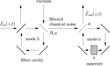
Figure 4: Sketch of the finite bandwidth classical noise source and squeezer.

Figure 5 presents results from the simulated measurement of $h_{\rm Y}(\tau)$, where figures 5(a) and (d) correspond to figures 2(b) and (c), respectively. The shot noise contribution to the central spike has disappeared while the contribution from the classical noise remains; for vacuum state squeezing there is no spike at all. Thus, vacuum state squeezing is distinguished qualitatively by the measurement from squeezed classical noise.

Figure 5: The correlation function $h_{\rm Y}(\tau)$ calculated for the model of figure 4: with classical noise bandwidth $B_{\rm c}=15$, detection bandwidth $B_{\rm d}=25$, DPO pump parameter $\lambda=0.4$, and classical noise photon number in the DPO cavity $\bar{n}_{a}=0.2$ (a), $\bar{n}_{a}=0.1$ (b), $\bar{n}_{a}=0.05$ (c), and $\bar{n}_{a}=0$ (d).

4 Conditional homodyne detection in stochastic electrodynamics

We turn now to our subsidiary theme. Given the comparison between figure 5 and figures 2(b) and (c), what does conditional homodyne detection have to say about realistic vacuum fluctuations—about stochastic electrodynamics?

Consider again our argument in section 3.3 for the disappearance of the shot noise spike. It regards the shot noise to be produced in the photoelectric detection process: shot noise is not derived from a fluctuation of the field and is therefore distinguishable from the classical noise which is. It appears then that stochastic electrodynamics suffers a fatal blow from the demonstrated results, as it sees shot noise precisely as additional (indistinguishable) fluctuations added to the field. Such a conclusion is too hasty, though. Stochastic electrodynamics does a better job of describing conditional homodyne detection than one might initially expect. Certainly it meets with difficulties of the usual sort. Nevertheless, it also predicts the vanishing of the shot noise spike; it offers an entirely different explanation of the effect. We conclude by modeling the conditional measurement of squeezing within stochastic electrodynamics.

The Achilles heel of stochastic electrodynamics is its inability to give a plausible account of the firing of photoelectric detectors. To avoid this important yet distracting issue, we set aside a consideration of the detection process itself and return to the attitude taken in section 2; we simply calculate moments of the measured fields. The arrangement used is illustrated in figure 6. There are three fields to consider:

$${\cal E}_{1}(t) = \left[{\cal E}_{\rm lo}\exp(-\rmi\omega_{0}t)+\sqrt{1-r}\mkern 2.0mu{\cal E}_{\rm out}(t)-\sqrt{r}\mkern 2.0mu{\cal E}_{\rm vac}(t)\right]/\sqrt{2},$$ (4.1)

$${\cal E}_{2}(t) = \left[{\cal E}_{\rm lo}\exp(-\rmi\omega_{0}t)-\sqrt{1-r}\mkern 2.0mu{\cal E}_{\rm out}(t)+\sqrt{r}\mkern 2.0mu{\cal E}_{\rm vac}(t)\right]/\sqrt{2},$$ (4.2)

and

$${\cal E}_{\rm start}(t)=\sqrt{r}\mkern 2.0mu{\cal E}_{\rm out}(t)+\sqrt{1-r}\mkern 2.0mu{\cal E}_{\rm vac}(t),$$ (4.3)

where $r$ is the reflection coefficient of beam splitter ${\rm BS}_{2}$ (figure 6) and

$${\cal E}_{\rm vac}(t)\equiv{\cal E}_{\rm vac}(z_{v},t),$$ (4.4)

$z_{v}$ an arbitrary location. Each field is filtered, with bandwidth $B_{\rm d}\kappa$, so that the vacuum fluctuations have finite photon flux. We calculate the correlation function as

$$h^{\prime}_{\rm Y}(\tau)=\frac{\overline{|{\cal E}_{\rm start}^{\prime}(0)|^{2}[|{\cal E}_{1}^{\prime}(\tau)|^{2}-|{\cal E}_{2}^{\prime}(\tau)|^{2}]}}{\overline{|{\cal E}_{\rm start}^{\prime}(0)|^{2}}\times\overline{[|{\cal E}_{1}^{\prime}(0)|^{2}-|{\cal E}_{2}^{\prime}(0)|^{2}]}};$$ (4.5)

${\cal E}_{1}^{\prime}(t)$, ${\cal E}_{2}^{\prime}(t)$, and ${\cal E}_{\rm start}^{\prime}(t)$ are the filtered fields. The question for us now is the following: what does this expression have to say about the shot noise spike?

In stochastic electrodynamics the signal field ${\cal E}_{\rm out}(t)$ carries realistic vacuum fluctuations, injected at the vacuum input to the filter cavity (figure 4). If this were the only vacuum input, the spike would remain in $h^{\prime}_{\rm Y}(\tau)$; but conditional detection introduces a second vacuum input—the field ${\cal E}_{\rm vac}(z,t)$ injected at beam splitter ${\rm BS}_{2}$. Considering it, the expansion of equation (4.5) (for Gaussian fluctuations) yields

$$h^{\prime}_{\rm Y}(\tau)=1+A\left[\overline{\tilde{\cal E}_{\rm out}^{\rm Y}(0)\tilde{\cal E}_{\rm out}^{\rm Y}(\tau)}-\overline{\tilde{\cal E}_{\rm vac}^{\rm Y}(0)\tilde{\cal E}_{\rm vac}^{\rm Y}(\tau)}\right],$$ (4.6)

where $A$ is a constant that depends on the amplitude of the offset $|{\cal E}_{\rm off}^{\prime}|$, the reflection coefficient $r$, and the filter bandwidth $2B_{\rm d}\kappa$. We see that the shot noise contribution to the spike is eliminated, not through the normal ordering of quantum operators, but by the explicit subtraction of the autocorrelation of the realistic vacuum fluctuations fed through beam splitter ${\rm BS}_{2}$, the term $-\overline{\tilde{\cal E}_{\rm vac}^{\rm Y}(0)\tilde{\cal E}_{\rm vac}^{\rm Y}(\tau)}$ [26].

Figure 6: The field arrangement used to model conditional homodyne detection in stochastic electrodynamics.

Figure 7: The correlation function $h^{\prime}_{Y}(\tau)$ calculated within stochastic electro-dynamics: for the parameters of figure 5.

Simulated results for $y_{\rm Y}^{\prime}(\tau)$ are presented in figure 7. They are in qualitative agreement with figure 5; although all is not well at a quantitative level; there is a difference in both the absolute and relative sizes of the squeezing dips. This comes from the inevitable difficulties faced by stochastic electrodynamics. A problem arises due to the presence in $|{\cal E}_{\rm start}(t)|^{2}$ of a nonphysical vacuum field photon flux proportional to the filter bandwidth $2B_{\rm d}\kappa$—i.e., nonphysical dark counts at the “start” detector. If we are prepared to set this inevitable problem aside, however, stochastic electrodynamics provides an alternative explanation for the elimination of the shot noise spike.

5 Conclusions

We have compared conditional and nonconditional measurements of quadrature squeezing and shown that conditional detection distinguishes qualitatively between quantum and classical squeezing. We showed that both measurements may be understood at a superficial level by adding realistic vacuum fluctuations to asymptotic input fields (stochastic electrodynamics). The strategy is unable to offer a plausible treatment of photoelectric detection, however, and this leads to serious quantitative errors in the treatment of the conditional measurement.

References

References

- [1] Special issue on “Squeezed Light” 1987 J. Mod. Opt. 34 709
- [2] Feature ussue on “Squeezed States of the Electromagnetic Field” 1987 J. Opt. Soc. Am. B 4 1450
- [3] Special issue on squeezed light 1992 Appl. Phys. B 4 189
- [4] Fabre C 1997 Quantum Fluctuations editors Reynaud S, Giacobino E and Zinn-Justin J (Amsterdam: North Holland) p 181
- [5] Pereira S F, Breitenbach G, Schiller S and Mlynek J 1997 Quantum Fluctuations editors Reynaud S, Giacobino E and Zinn-Justin J (Amsterdam: North Holland) p 267
- [6] Furusawa A, Sørensen J L S, Braunstein S L, Fuchs C A, Kimble H J and Polzik E S 1998 Science 282 706
- [7] Bowen W P, Treps N, Buchler B C, Schnabel R, Ralph T C, Bachor H-A, Symul T and Lam P K 2003 Phys. Rev. A 67 032302
- [8] Yuen H P and Chan V W S 1983 Opt. Lett. 8 177
- [9] Carmichael H J, Castro-Beltran H M, Foster G T and Orozco L A 2000 Phys. Rev. Lett. 85 1855
- [10] Foster G T, Orozco L A, Castro-Beltran H M, and Carmichael H J 2000 Phys. Rev. Lett. 85 3149
- [11] Dalton B ?, Ficek ? ?, and Swain S 1999 J. Mod. Opt. 46, 379
- [12] Yurke B 1984 Phys. Rev. A 29 408
- [13] Caves C M and Schumaker B L 1985 Phys. Rev. A 31 3068
- [14] Schumaker B L and Caves C M 1985 Phys. Rev. A 31 3093
- [15] Carmichael H J 1999 Statistical Methods in Quantum Optics 1: Master Equations and Fokker-Planck Equations (Berlin: Springer-Verlag) p 108
- [16] Marshall T W 1963 Proc. R. Soc. London 276 475
- [17] Boyer T H 1975 Phys. Rev. D 11 809
- [18] Marshall T W and Santos E 1988 Found. Phys. 18 185
- [19] Casado A, Marshall T W and Santos E 1997 J. Opt. Soc. Am. B 14 494
- [20] Casado A, Fernández-Rueda A, Marshall T W, Risco-Delgado R and Santos E 1997 Phys. Rev. A 55 879
- [21] Casado A, Fernández-Rueda A, Marshall T W, Risco-Delgado R and Santos E 1997 Phys. Rev. A 56 477
- [22] Casado A, Marshall T W and Santos E 1998 J. Opt. Soc. Am. B 15 1572
- [23] Carmichael H J 1993 An Open Systems Approach to Quantum Optics Lecture Notes in Physics vol m18 (Berlin: Springer-Verlag) p 140
- [24] Foster G T, Smith W P, Reiner J E and Orozco L A 2002 Phys. Rev. A 66 33807
- [25] Carmichael H J 1993 Phys. Rev. Lett. 70 2273
- [26] A similar subtraction to that in equation (4.6) is made in equation (12) of Ralph T C, Munro W J, and Polkinghorne R E S 2000 Phys. Rev. Lett. 85, 2035