Proposed Test of Quantum Nonlocality for Continuous Variables

Abstract

We propose a test of nonlocality for continuous variables using a two-mode squeezed state as the source of nonlocal correlations and a measurement scheme based on conditional homodyne detection. Both the CHSH- and the CH-inequality are constructed from the conditional homodyne data and found to be violated for a squeezing parameter larger than $r\approx 0.48$.

Nonlocality has been a topic of great interest ever since Bell reevaluated the claim of Einstein, Podolsky, and Rosen (EPR) that quantum mechanics is incomplete Bell1 . Considerable effort has been invested in experimental demonstrations of nonlocality, which manifests itself through the violation of a Bell inequality. Experiments for discrete variable systems have used the polarization state of photon pairs in an atomic cascade Aspect or parametric down conversion Zeilinger , and the spin state of trapped ions Rowe . Experiments for continuous variable (CV) systems have been rare; although they are of particular interest as they match more closely the situation considered in the original work of EPR. Recently, A. Kuzmich et al. Kuzmich reported a signature of nonlocality in an intensity correlation measurement of a pulsed mode EPR state. These authors adopt the approach proposed by Grangier et al. Grangier , whereby an auxiliary constraint is imposed to construct the relevant Bell inequality. Specifically, it is assumed in this case that a change in local oscillator phase does not change the total detection probability in the transmitted and reflected channels.

The EPR state, or in quantum optics, the two-mode squeezed state, plays a central role in the quantum information processing of CVs QIbook . It is not possible, however, to demonstrate nonlocality for the EPR state directly by making a CV measurement, since the EPR state (more generally any Gaussian state) possesses a positive-definite Wigner function, which provides a hidden variable model Bell . For this reason, proposals for demonstrating nonlocality with EPR-like states (squeezed states) employ dichotomous observables derived from some discrete physical characteristic, e.g. even and odd photon number. In this way it is possible to formally map the CV system onto a spin-1/2 Chen . Alternatively, Banaszek and Wodkiewicz demonstrated that the Bell inequality constructed from a joint parity measurement (photon number even or odd) is violated for two-mode squeezed states Banaszek . They provide an operational connection between their scheme and the Wigner phase-space distribution. These proposals suffer from two limitations, however: first, being based on discrete data sets, they do not demonstrate nonlocality of a true continuous character; they are also difficult to realize experimentally, due to the inefficiency of photoelectric detection. Another strategy is to retain the CV measurement in the form of balanced homodyne detection—a highly efficient measurement compared to photon counting—but consider a non-Gaussian state Leonhardt . Offsetting the fundamental merit of this approach is the difficulty of preparing the states shown to exhibit nonlocality to date Leonhardt ; Gilchrist ; Munro .

In this Letter we show that the optical EPR state (two-mode squeezed state), although possessing a positive Wigner function, provides for a genuine CV nonlocality test under conditional homodyne detection, where collection of the homodyne data is conditioned on the prior local detection of one or more photons by each of the parties sharing the EPR-correlated fields. The detection scheme is motivated by the work of Foster et al. Foster . Although the detection is conditional, the demonstrated violation of locality may still be attributed to the EPR state itself, since local detection of a photon cannot create nonlocal correlations from a classically correlated state.

Ralph et al. Ralph1 also proposed a scheme demonstrating Bell-type correlations using homodyne detection of two-mode squeezed states and an auxiliary measurement; but their scheme imposes a constraint on the considered hidden-variable models Ralph2 , in a similar manner to Refs. Kuzmich ; Grangier . In contrast, the underlying principle of our proposal is that conditioning on the detection of a photon is a nonlinear operation that transforms a Gaussian state into a non-Gaussian one; thus, the conditioning automatically prepares a state that does not possess a positive-definite Wigner function. The demonstrated nonlocality may be attributed to the newly prepared state. Our scheme therefore constitutes a genuine CV nonlocality test, and demonstrates a violation of the Bell inequality in the strong sense, with no additional constraint on the considered hidden-variable models Note1 . We show that it is insensitive to the quantum efficiency of the detectors that generate the conditioning photocounts.

The proposed scheme is depicted in Fig. 1. Light in a two-mode squeezed state $\rho_{12}$ is spatially separated and mixed with the vacuum field—states $|0\rangle\langle 0|_{3,4}$—at beam splitters of reflectance $R=\sin^{2}\theta$. Balanced homodyne detection is performed at output ports $1$ and $2$, with local oscillator phases $\phi_{1}$ and $\phi_{2}$, respectively, as shown in the figure. Photodetectors ${\rm PD}_{3}$ and ${\rm PD}_{4}$ register photon counts, at output ports $3$ and $4$, respectively. The photodetectors merely detect the presence of photons, and hence output modes $3$ and $4$ are projected to states of either zero or any nonzero photon number, according to the detection record. Data from the balanced homodyne detectors, ${\rm HD}_{1}(\phi_{1})$ and ${\rm HD}_{2}(\phi_{2})$, are collected only when both ${\rm PD}_{3}$ and ${\rm PD}_{4}$ fire. The conditional state presented for homodyne measurement is therefore

$$\rho_{c}=\frac{{\rm tr}_{34}\{\rho_{\rm BS}\hat{P}_{3}\hat{P}_{4}\}}{{\rm tr}\{\rho_{\rm BS}\hat{P}_{3}\hat{P}_{4}\}},$$ (1)

with $\hat{P}_{i}=I_{i}-|0\rangle\langle 0|_{i}$ ($i=3,4$) and

$$\rho_{\rm BS}=\hat{B}_{13}^{{\dagger}}\hat{B}_{24}^{{\dagger}}\big{(}\rho_{12}\otimes|0\rangle\langle 0|_{34}\big{)}\hat{B}_{13}\hat{B}_{24},$$ (2)

where $\hat{B}_{ij}^{{\dagger}}=\exp[(\theta-\pi/2)(\hat{a}_{i}^{{\dagger}}\hat{a}_{j}-\hat{a}_{i}\hat{a}_{j}^{{\dagger}})]$ accounts for the beam splitter action.

Figure 1: Schematic diagram of the conditional homodyne detection of an EPR-correlated state. Two beams of light in the correlated state $\rho_{12}$ are shared at beam splitters ${\rm BS(\theta)}$ between photodetectors ${\rm PD}_{3}$ and ${\rm PD}_{4}$, and homodyne detectors ${\rm HD}_{1}(\phi_{1})$ and ${\rm HD}_{2}(\phi_{2})$. The homodyne data is accepted when both photodetectors fire (each at least once).

To construct a CHSH inequality we use a binning process to convert the continuous homodyne date into binary form. We adopt the scheme used by Bell Bell and Gilchrist et al. Gilchrist , assigning a value $+1$ ($-1$) when a measurement of the quadrature variable ${\hat{x}}_{\phi}\equiv\frac{1}{2}\left(\hat{a}e^{-i\phi}+\hat{a}^{{\dagger}}e^{i\phi}\right)$ gives a nonnegative (negative) result. In the single mode case, the probability for a nonnegative result is given by

$$P_{+}(\phi)=\int_{-\infty}^{\infty}dx_{\phi}\mkern 2.0mup(x_{\phi})\theta(x_{\phi})=\langle{\hat{\theta}}\left({\hat{x}}_{\phi}\right)\rangle,$$ (3)

with

$${\hat{\theta}}\left({\hat{x}}_{\phi}\right)\equiv\frac{1}{\pi}\mkern-2.0mu\int_{0}^{\infty}\mkern-2.0mudy\mkern-2.0mu\int_{-\infty}^{+\infty}\mkern-2.0mudk\mkern 2.0mue^{2ik({\hat{x}}_{\phi}-y)};$$ (4)

$\hat{\theta}(\hat{x})$ is the operator step function, with $\theta(x)=1$ or $0$, for $x\geq 0$ or $x<0$. The two-mode probability, $P_{++}\left(\phi_{1},\phi_{2}\right)$, that measurements of ${\hat{x}}_{\phi_{1}}$ at output 1 and ${\hat{x}}_{\phi_{2}}$ at output 2 both yield nonnegative results is given by

$$P_{++}\left(\phi_{1},\phi_{2}\right) = {\rm tr}\{\rho{\hat{\theta}}_{1}\left({\hat{x}}_{\phi_{1}}\right){\hat{\theta}}_{2}\left({\hat{x}}_{\phi_{2}}\right)\}$$ (5)

$$= \frac{1}{\pi^{2}}\mkern-2.0mu\int\mkern-2.0mud^{2}y\mkern-2.0mu\int\mkern-2.0mud^{2}k\mkern 2.0muC\left(\xi_{1},\xi_{2}\right)e^{-2i{\bm{k}}\cdot{\bm{y}}},$$

with ${\bm{y}}\equiv(y_{1},y_{2})$, ${\bm{k}}\equiv(k_{1},k_{2})$, and $\xi_{i}=ik_{i}e^{i\phi_{i}}$ ($i=1,2$), where

$$C\left(\lambda_{1},\lambda_{2}\right)\equiv{\rm tr}\{\rho_{c}\hat{D}_{1}(\lambda_{1})\hat{D}_{2}(\lambda_{2})\}$$ (6)

is the characteristic function of the two-mode state $\rho_{c}$, with $\hat{D}_{i}(\lambda_{i})\equiv\exp(\lambda_{i}\hat{a}_{i}^{{\dagger}}-\lambda^{*}_{i}\hat{a}_{i})$ the displacement operator; integration with respect to ${\bm{y}}$ and ${\bm{k}}$ in Eq. (5) covers the positive quadrant and the entire plane, respectively. Introducing the two-mode Wigner function $W_{12}\left(\alpha_{1},\alpha_{2}\right)$ [the Fourier transform of $C(\lambda_{1},\lambda_{2})$] Eq. (5) yields

$$P_{++}\left(\phi_{1},\phi_{2}\right)$$

$$=\int\mkern-2.0mud^{2}\mkern-2.0mu\alpha_{1}\mkern-2.0mu\int d^{2}\mkern-2.0mu\alpha_{2}W_{12}\left(\alpha_{1},\alpha_{2}\right)F\left(\alpha_{1},\phi_{1}\right)F\left(\alpha_{2},\phi_{2}\right),\mkern 30.0mu$$ (7)

where $F\left(\alpha,\phi\right)\equiv\theta\left({\rm Re}\{\alpha e^{i\phi}\}\right)$. It is clear from this equation that if the Wigner function is positive definite, the amplitudes $\alpha_{1},\alpha_{2}$ provide a hidden variable explanation of any correlation revealed by $P_{++}\left(\phi_{1},\phi_{2}\right)$ .

We find it most practical to calculate $P_{++}\left(\phi_{1},\phi_{2}\right)$ from Eq. (5), where we first calculate the characteristic function (6). Denoting the probability of joint photodetection by $p_{34}={{\rm tr}\{\rho_{\rm BS}\hat{P}_{3}\hat{P}_{4}\}}$ and using the normal-ordered form $|0\rangle\langle 0|_{i}={:\exp({-\hat{a}_{i}^{{\dagger}}\hat{a}_{i}}):}$, after some algebra we find

$$C\left(\lambda_{1},\lambda_{2}\right) = p_{34}^{-1}C_{\rm vac}\left(-\lambda_{1}\cos\theta\right)C_{\rm vac}\left(-\lambda_{2}\cos\theta\right)$$ (8)

$$\times{\rm tr}\left\{\rho^{\prime}_{12}\hat{D}_{1}(\lambda_{1}\sin\theta)\hat{D}_{2}(\lambda_{2}\sin\theta)\right\},$$

where $C_{\rm vac}\left(\lambda\right)=e^{-|\lambda|^{2}/2}$ is the characteristic function of the single-mode vacuum, and

$$\rho^{\prime}_{12}=\left({\cal I}_{1}-{\cal S}_{1\theta}\right)\otimes\left({\cal I}_{2}-{\cal S}_{2\theta}\right)\rho_{12};$$ (9)

superoperators $S_{1\theta}$ and $S_{2\theta}$ are defined by

$${\cal S}_{i\theta}\equiv\sum_{k=0}^{\infty}\frac{(-\cos^{2}\theta)^{k}}{k!}\mkern 2.0mu\hat{a}_{i}^{k}\cdot\mkern 2.0mu\hat{a}_{i}^{{\dagger}k},$$ (10)

while ${\cal I}_{1}$ and ${\cal I}_{2}$ are superoperator identities. The probability $p_{34}$ is obtained by setting $\lambda_{1}=\lambda_{2}=0$ in Eq. (8).

The mapping $\cal M$ defined by Eqs. (8) and (9) has some notable features. First, it preserves local classicality, in the sense that a state that is locally classical in view of its Glauber P-function is mapped to another such state. Second, and more importantly, it is a nonlinear operation $\left({\cal M}\{\Sigma_{i}p_{i}\rho_{12}^{i}\}\neq\Sigma_{i}p_{i}{\cal M}\{\rho_{12}^{i}\}\right)$ that transforms a Gaussian state to a non-Gaussian one. In particular, a two-mode squeezed state is mapped to a state which does not possess a positive-definite Wigner function. We note, for example, that the Wigner function of any single-mode field with zero vacuum component necessarily takes negative values, since it must satisfy $\langle 0|\rho|0\rangle=2\!\int\!d^{2}\alpha\,W(\alpha)e^{-2|\alpha|^{2}}=0$. Thus, in spite of the undesirable contamination by the vaccum states in Eq. (8), a nonlocality test by a CV measurement becomes possible.

The two-mode squeezed state adopted for the input is

$$\rho_{12}=\frac{1}{\pi^{2}}\mkern-2.0mu\int\mkern-2.0mud^{2}\lambda_{1}\mkern-2.0mu\int\mkern-2.0mud^{2}\lambda_{2}C_{\rm sq}\left(\lambda_{1},\lambda_{2}\right)\hat{D}_{1}^{{\dagger}}(\lambda_{1})\hat{D}_{2}^{{\dagger}}(\lambda_{2}),$$ (11)

with characteristic function

$$C_{\rm sq}\left(\lambda_{1},\lambda_{2}\right) = \exp\mkern-2.0mu\left[-{\textstyle\frac{1}{2}\displaystyle}\cosh 2r(|\lambda_{1}|^{2}+|\lambda_{2}|^{2})\right.$$ (12)

$$+\left.\vphantom{\textstyle\frac{1}{2}\displaystyle}\sinh 2r{\rm Re}(\lambda_{1}\lambda_{2}^{*})\right],$$

where $e^{-2r}$ is the degree of squeezing. A long but straightforward calculation using Eqs. (5) and (8) then gives the binning probability

$$P_{++}\left(\phi_{1},\phi_{2}\right)=\frac{1}{4}+\frac{1}{2\pi p_{34}}\sum_{i=1}^{3}c_{i}\mkern-2.0mu\tan^{-1}\mkern-2.0mu\left[\frac{A}{\sqrt{b_{i}^{2}-A^{2}}}\right]\mkern-2.0mu,\mkern 10.0mu$$ (13)

with $A=\sin^{2}\theta\sinh 2r\cos(\phi_{1}+\phi_{2})$,

$$b_{1} = 1+2\sin^{2}\theta\sinh^{2}r,$$

$$b_{2} = \sqrt{d_{1}d_{2}},$$

$$b_{3} = b_{1}+\eta(2-\eta)\cos^{4}\theta\sinh^{2}r,$$ (14)

and

$$c_{1} = 1$$

$$c_{2} = -2(1+d_{1}-b_{1})^{-1},$$

$$c_{3} = (1+b_{3}-b_{1}+d_{1}-d_{2})^{-1}$$

$$d_{1} = b_{1}+\eta\cos^{2}\theta\sinh^{2}r,$$

$$d_{2} = d_{1}-2\eta\sin^{2}\theta\cos^{2}\theta\sinh^{2}r.$$ (15)

These expressions take into account the nonunit quantum efficiency $\eta$ of the photodetectors at outputs 3 and 4. The joint photodetection probability is found to be

$$p_{34}=\frac{B^{2}{\rm tanh}^{2}r\left[1+(1-B){\rm tanh}^{2}r\right]}{\left[1-(1-B){\rm tanh}^{2}r\right]\mkern-3.0mu\left[1-(1-B)^{2}{\rm tanh}^{2}r\right]},$$ (16)

with $B=\eta\cos^{2}\theta$. The local probability that homodyne detection gives a nonnegative result is $P_{i+}(\phi_{i})=1/2$ ($i=1,2$), independent of the phase $\phi_{i}$.

We note that $P_{++}\left(\phi_{1},\phi_{2}\right)$ depends only on the sum of local oscillator phases $\phi_{1}+\phi_{2}$, which we denote $\phi$. Because $P_{--}\left(\phi_{1},\phi_{2}\right)=P_{++}\left(\phi_{1},\phi_{2}\right)$ in the present case, the correlation

$$E\left(\phi_{1},\phi_{2}\right) \equiv P_{++}(\phi_{1},\phi_{2})+P_{--}(\phi_{1},\phi_{2})$$ (17)

$$-P_{+-}(\phi_{1},\phi_{2})-P_{-+}(\phi_{1},\phi_{2})$$

that enters the CHSH inequality CHSH can be evaluated from $P_{++}\left(\phi_{1},\phi_{2}\right)$ alone, and hence is also a function of $\phi$ only. We write

$$E(\phi)\equiv E(\phi_{1},\phi_{2})=4P_{++}(\phi_{1},\phi_{2})-1,$$ (18)

and the CHSH inequality is written as

$$B_{\rm CHSH}\equiv|E(\phi)-E(\varphi)+E(\varphi^{\prime})+E(\phi^{\prime})|\leq 2.$$ (19)

The inequality must be satisfied for any $\phi=\phi_{1}+\phi_{2}$, $\phi^{\prime}=\phi^{\prime}_{1}+\phi^{\prime}_{2}$, $\varphi=\phi^{\prime}_{1}+\phi_{2}$, and $\varphi^{\prime}=\phi_{1}+\phi^{\prime}_{2}$.

With the phases set to $\phi=\phi^{\prime}=\varphi/3=-\varphi^{\prime}\equiv\Psi$, the optimal violation occurs at $\Psi=\pi/4$. To realize this setting, we might take, for example, $\phi_{1}=0$, $\phi^{\prime}_{1}=\pi/2$, and $\phi_{2}=-\phi^{\prime}_{2}=\pi/4$. Adopting these values, in Fig. 2 the quantity $B_{\rm CHSH}$ is plotted as a function of the squeezing parameter $r$ and reflectance $R=\sin^{2}\theta$ (for $\eta=1$). Violation of the CHSH inequality occurs for any $r$ larger than $r\approx 0.48$ so long as the reflectance is sufficiently large. The need for a sufficiently large reflectance is to be expected, since too low a reflectance contaminates the outputs with the vacuum field from inputs 3 and 4 [Eq. (8)]. The maximal violation occurs for $r\approx 0.65$, with a decreasing violation at larger values of $r$. The appearance of such a maximum is expected also, as the mean photon number increases with the squeezing $r$, and at large photon numbers the projections $P_{i}=I_{i}-|0\rangle\langle 0|_{i}$ ($i=3,4$) bring little change to the input Gaussian state. The expected behavior is reflected in the fact that the joint photocount probability [Eq. (16)] approaches unity for $r\rightarrow\infty$—i.e., the conditioning is no longer selective.

We note that whenever the CHSH inequality is violated, the strong CH inequality is violated also, as was found in Munro . According to the latter,

$$B_{\rm CH}\equiv\frac{P_{++}\left(\phi\right)-P_{++}\left(\varphi\right)+P_{++}\left(\varphi^{\prime}\right)+P_{++}\left(\phi^{\prime}\right)}{P_{1+}(\phi^{\prime}_{1})+P_{2+}(\phi_{2})}$$ (20)

is bounded by unity for any local realistic model Clauser . In our case, $P_{1+}(\phi^{\prime}_{1})=P_{2+}(\phi_{2})=1/2$, and hence $4B_{\rm CH}=\left(B_{\rm CHSH}+2\right)$, from Eqs. (18)–(20). Thus, $B_{\rm CHSH}>2$ is equivalent to $B_{\rm CH}>1$.

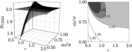
Figure 2: $B_{\rm CHSH}$ as a function of the squeezing parameter $r$ and the reflectance $R=\sin^{2}\theta$, for quantum efficiency $\eta=1$. The CHSH inequality is violated for $B_{\rm CHSH}>2$.

As discussed in Gilchrist , homodyne detection with a strong LO is highly efficient compared to direct photon counting. But unlike the proposal there, our proposal relies on photodetectors ${\rm PD}_{3}$ and ${\rm PD}_{4}$ in addition to the homodyne detectors ${\rm HD}_{1}$ and ${\rm HD}_{2}$ (Fig. 1). It is important, therefore, to investigate the dependence of our results on the quantum efficiency of these detectors. To obtain expressions (13)–(16), a nonunit quantum efficiency was introduced by mixing outputs 3 and 4 with additional vacuum states, placing beam splitters of transmittance $\eta$ in front of ${\rm PD}_{3}$ and ${\rm PD}_{4}$. From a direct calculation, the term $\cos^{2}\theta$ in Eq. (10) is replaced by $\eta\cos^{2}\theta$, with no further change required in Eq. (8). Figure 3(a) presents a contour plot of $B_{\rm CHSH}$ as a function of $r$ and $R=\sin^{2}\theta$ for a quantum efficiency $\eta=0.3$. Comparing Fig. 2, we see that the violation of the CHSH inequality is not especially sensitive to $\eta$. In particular, when $R$ is close to unity, as in Fig. 3(b), $B_{\rm CHSH}$ hardly changes with $\eta$ at all; here the CHSH inequality is violated for any quantum efficiency. Of course, a high efficiency is desirable to maximize the rate of data acquisition, which is determined by the joint photocount probability $p_{34}$.

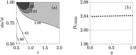
Figure 3: (a) $B_{\rm CHSH}$ as a function of the squeezing parameter $r$ and the reflectance $R=\sin^{2}\theta$, for quantum efficiency $\eta=0.3$. (b) $B_{\rm CHSH}$ as a function of $\eta$, for $r=0.6$ and $R\approx 0.9891$.

Realization of the proposed scheme appears to be feasible with currently available methods. The EPR paradox for CVs has been demonstrated with squeezed light Ou , and EPR-correlated light has been used for the quantum teleportation of coherent states Furusawa . These particular experiments involve multimode fields, however, and it will be necessary to generalize the present treatment for application to that case. More relevant to this work is the experiment of Kuzmich et al. Kuzmich , where the optical analog of the EPR state is produced in a pulsed optical parametric amplifier. In such a case the projections associated with photodetectors ${\rm PD}_{3}$ and ${\rm PD}_{4}$ refer to the total photon number in a single spatio-temporal mode.

Finally, we should comment on the subtle question of whether the proposed conditional test demonstrates nonlocality for the initial state $\rho_{12}$. The most important observation in this regard is that the sampling of the homodyne data is based on the local detection of photons coming from inputs 1 and 2. How observers of ${\rm PD}_{3}$ and ${\rm PD}_{4}$ determine whether to keep or discard the data involves, at most, a classical communication. Thus, the act of conditional data acquisition cannot create nonlocality from a classically correlated state; this is clearly reflected in the tensor product form of Eq. (9). In this sense, one may argue that the demonstrated nonlocality is implicitly an attribute of the initial state $\rho_{12}$. In particular, the situation differs from the so-called “detection loophole” Rowe , which asserts that “unfair” data sampling can lead to the violation of a Bell inequality even for a classically correlated state. In our case the data sampling is “fair” and under the experimenter’s control.

Of course, this is not to claim that the proposed test demonstrates nonlocality for $\rho_{12}$ directly. Strictly, a new state having a CV nonlocal correlation is created by the conditioning [Eq. (8)] and homodyne detection is used to reveal nonlocality for the newly created state.

In conclusion, we have shown that nonlocality for CVs can be demonstrated by conditional homodyne detection, where the optical analog of the orginal EPR state (two-mode squeezed state) provides the source of nonlocal correlations. Violation of the CHSH inequality occurs for squeezing parameters greater than $r\approx 0.48$, and the proposed scheme is insensitive to the quantum efficiency of the conditioning photodetectors. In addition, our work has broader relevance to the field of quantum information. It shows that even a positive Wigner-function state can be employed as a source of continuous-variable nonlocality if suitable local nonlinear operations are added. It provides a concrete example of the “photon-presence test” performing such an operation Bartlett .

This work was supported by the NSF under Grant No. PHY-0099576 and by the Marsden Fund of the RSNZ. Email: hnha001@postbox.auckland.ac.nz

References

- (1) J. S. Bell, Physics ( N. Y.), 1, 195 (1965).
- (2) S. J. Freedman et al., Phys. Rev. Lett. 28, 938 (1972); A. Aspect et al., Phys. Rev. Lett. 49, 91 (1982).
- (3) P. G. Kwiat et al., Phys. Rev. Lett. 75, 4337 (1995); G. Weihs et al., Phys. Rev. Lett. 81, 5039 (1998).
- (4) M. A. Rowe et al., Nature 409, 791 (2001).
- (5) A. Kuzmich et al, Phys. Rev. Lett. 85, 1349 (2000).
- (6) P. Grangier et al., Phys. Rev. A38, R3132 (1988).
- (7) Quantum Information with Continuous Variables, edited by S. L. Braunstein and A. K. Pati, (Kluwer, Dordrecht, 2003)
- (8) J. S. Bell, Speakable and Unspeakable in Quantum Mechanincs, (Cambridge University Press, Cambridge, 1987), Chap. 21.
- (9) Z.-B. Chen et al., Phys. Rev. Lett. 88, 40406 (2002).
- (10) K. Banaszek and K. Wodkiewicz, Phys. Rev. A58, 4345 (1998); Phys. Rev. Lett. 82, 2009 (1999).
- (11) U. Leonhardt et al., J. Mod. Opt 42, 939 (1995).
- (12) A. Gilchrist et al., Phys. Rev. Lett. 80, 3169 (1998).
- (13) W. J. Munro, Phys. Rev. A59, 4197 (1999).
- (14) G. T. Foster et al., Phys. Rev. Lett. 85, 3149 (2000).
- (15) T. C. Ralph et al., Phys. Rev. Lett. 85, 2035 (2000); T. C. Ralph and W. J. Munro, quant-ph/0104092.
- (16) E. H. Huntington and T. C. Ralph, Phys. Rev. A65, 012306 (2001).
- (17) It is questionable whether proposal Ralph1 demonstrates nonlocality of a genuine continuous character, since it merely reexpresses what is fundamantally a photon-counting inequality in terms of homodyne detection.
- (18) J. F. Clauser et al., Phys. Rev. Lett. 23, 880 (1969).
- (19) J. F. Clauser et al., Phys. Rev. D10, 526 (1974).
- (20) Z. Y. Ou et al., Phys. Rev. Lett. 68, 3663 (1992).
- (21) A. Furusawa et al., Science 282, 706 (1998).
- (22) S. D. Bartlett et al., Phys. Rev. Lett. 89, 207903 (2002).