Quantum Dynamics of a Particle with a Spin-dependent Velocity

Abstract

We study the dynamics of a particle in continuous time and space, the displacement of which is governed by an internal degree of freedom (spin). In one definite limit, the so-called quantum random walk is recovered but, although quite simple, the model possesses a rich variety of dynamics and goes far beyond this problem. Generally speaking, our framework can describe the motion of an electron in a magnetic sea near the Fermi level when linearisation of the dispersion law is possible, coupled to a transverse magnetic field. Quite unexpected behaviours are obtained. In particular, we find that when the initial wave packet is fully localized in space, the $J_{z}$ angular momentum component is frozen; this is an interesting example of an observable which, although it is not a constant of motion, has a constant expectation value. For a non-completely localized wave packet, the effect still occurs although less pronounced, and the spin keeps for ever memory of its initial state. Generally speaking, as time goes on, the spatial density profile looks rather complex, as a consequence of the competition between drift and precession, and displays various shapes according to the ratio between the Larmor period and the characteristic time of flight. The density profile gradually changes from a multimodal quickly moving distribution when the scatttering rate is small, to a unimodal standing but flattening distribution in the opposite case.

I Introduction

The term quantum random walk has been coined some times ago by Aharonov and Davidovich Aharonov to qualify the motion of a quantum particle moving either left or right according to the value of the $J_{z}$ component of its spin. As such, this is completely different of the quantum Brownian motion problem, in which one fully describes in a quantum framework the motion of a single (light) particle moving in a bath of heavy particles – a quantum version of the classical Brownian motion. This latter problem has been the subject of many papers in the past, revivified in the 80’s by the pioneering work of Caldeira and Leggett (for a review, see Leggett etal Caldelegggett ), showing that for the so-called ohmic coupling with the bath, dynamical symmetry breaking occurs above a given threshold. On a more elementary level, simple models show how the classical brownian motion can be generalized to the quantum world, although long time scales (and algebraic behaviours) appear in correlation functions at small enough temperature, as shown by Aslangul etal Asl85 . We shall adopt here the recent meaning as proposed by Aharonov and Davidovich, shortened as QRW in the following.

This latter problem is presently the subject of an intense activity, following the basic papers by Ambainis et al Ambainis01 , Nayak and Vishwanath nayak and Dür et al Duretal (for a recent comprehensive review, see the preprint by Kempe kempe081 ). The basic motivation lies in the fact that QRW yields a dynamics at the opposite of classical random walk: for a spin $\frac{1}{2}$ particle, and a symmetric initial spin state with definite phases (see below for details), the probability density in space $P_{\rm QRW}(x,\,t)$ displays two well-defined peaks, moving away linearly in time from the starting place. This is to be contrasted with the $t^{1/2}$ spreading of the classical packet, the particle staying (in the average) at its starting point when no drift is present. It can be said that QRW, except for oscillations in spatial density, displays the same basic features as the classical non-difffusive motion with a drift (which can be obtained from the biased diffusion equation $\frac{\partial P}{\partial t}=-\vec{\nabla}[\vec{v}\,P-D\vec{\nabla}\,P]$ – in the (singular) limit $D\rightarrow\,0$, as explained for instance in the book by Gardiner gardiner ) –, when the velocity itself is a random variable assuming two values $\pm v_{0}$ with definite probabilities. This rather intuitive picture has been firmly grounded by the recent work of Blanchard and Hongler blanchongler .

Due to the quantum nature of the walk, all steps are strongly correlated (as contrasted to classical motion), as it is also the case for repeated mesurements yielding the Zeno paradox theoretically found by Misra and Sudarshan misrasudar and observed by Itano et alitano ; this means that specific ever-lasting correlations are always relevant. One consequence is that the linear dimension of the visited space increases linearly in time, i. e. much more rapidly for QRW than for classical motion. It is hoped, on a somewhat speculative level, that Monte-Carlo algorithms could be improved by drawing benefit of this fact (see e. g. Kempe kempe0205 ).

We adopt here a more general point of view. Indeed, we define a simple model containing a single parameter, noted $\alpha$ in the following, which is essentially the product of the spin-flip rate by the time of flight in space. As shown below, the limit $\alpha\rightarrow\,0$ can be viewed as the continuous space-time version of the conventional QRW. Out this limiting case, the model can describe the dynamics of an electron near the Fermi level (once the dispersion law has been linearized, $\varepsilon(k)\rightarrow\,\pm\hbar(k-k_{\rm F})v_{\rm F}$ as is done e. g. in the Luttinger model luttinger ), moving in a magnetic sea created by impurities, or coupled to nuclear spins (Vagner vagner ). Elastic collisions with the magnetic background can flip the spin of the moving electron and, simultaneously, change its velocity from $+v_{\rm F}$ to $-v_{\rm F}$. Alternatively, such an reversal can be induced by a transverse magnetic field forcing the spin to precess harmonically at the Larmor frequency $\omega$. As a whole, spin and orbital degrees of freedom are coupled, yielding intrication of the state as time goes on, and competition between precession and translation in space. This produces interesting effects; the first one (and probably the most unexpected) is freezing of the precession when the initial packet is quite narrow – an effect which could have interesting applications in spintronics, as well in two-dimensional systems (McGuire et al mcguire ), in carbon nanotubes (Yang et al yang ), in quantum dots (Levitov and Rashba levitov ) and in semiconductors (Dyakonov dyakonov ). A second characteristic feature is the $\propto t$ spreading of the wavepacket which arises in any case, even when the precession is extremely rapid: because of the latter, the particle has no time to choose between right and left moves, but dispersion still occurs, and very quickly as compared to classical random motion.

Obviously, the physical relevance of our model is subjected to small deviations around $k_{\rm F}$. On the other side, it is hoped that the basic (and surprising) results found below keep some relevance even with such restrictions, and at least can take place on space and time scales to be precised in real life. It is worthy to note that, provided such a physical picture is meaningful, $\alpha$ becomes an easily tunable parameter by varying either the magnetic field, or the filling-ratio of the band, or the density of the magnetic diffusing centers.

This paper is organized as follows. We first define the model (section II), we explicitely show the relation between our model and QRW and we give a qualitative discussion of limiting cases. We then briefly derive the equations giving the time-evolution of the density for an arbitrary spin $J$ (section III), on which the spin-locking due to space confinement in the $\alpha\,\rightarrow\,0$ limit can be directly shown. This fact is confirmed by a detailed study of the average value $J_{z}$ (section IV). Then, we focus on the $J=\frac{1}{2}$ case (section V), and calculate the density profile $P(x,\,t)$, which displays many various shapes, some unexpected when the two time-scales related to the Larmor precession and the displacement in space are of the same order of magnitude. Eventually, conclusions are drawn and hints for future work are given. In the Appendix, details are given on the asymptotic analytical work required to get insight on the features of the probability density.

II Model and qualitative discusssion

For a spin $\vec{J}$ particle, our model Hamiltonian reads:

$$H\,=\,\omega J_{y}+\hbar^{-1}\vec{v}.\hat{\vec{p}}\,J_{z}\enspace.$$ (1)

In this expression, $\omega$ is the spin-flip rate due to scattering on impurities, or the Larmor frequency due to a transverse magnetic field along the $y$ direction. $\vec{v}$ is the (scalar) quantity defining the velocity-scale, $\hat{\vec{p}}$ is the momentum (${\hat{p}}=-{\rm i}\hbar\vec{\nabla}$ in the $q$-representation). Despite some similitude at first glance, the Hamiltonian (1) has nothing to do with the Dirac Hamiltonian, in which the momentum is coupled to the Dirac $\vec{\alpha}$ matrices; indeed, the angular momentum (spin) is there not given by $\vec{\alpha}$ and, in addition, the problem has here the dimensionality $2J+1$ in spin space, instead of four in the Dirac theory. Also note that, in its one-dimensional form, with a space dependent $\omega$ and for $J=\frac{1}{2}$, this Hamiltonian has been used in various contexts such as inhomogeneous supraconductors (de Gennes degennes ) and solitons in polyacetylene (Takayama et al makietal ).

In the following, we restrict to one-dimensional space; calling $Ox$ the line on which the particle moves, the Hamiltonian (1) simplifies to:

$$H=\omega J_{y}+\hbar^{-1}v\,{\hat{p}}\,J_{z}\enspace,\qquad{\hat{p}}\,=\,-{\rm i}\hbar\frac{\partial}{\partial x}\enspace.$$ (2)

Note that the label $x$ of direction of motion and the three directions defining the components $J_{x},\,J_{y}$ and $J_{z}$ generally have no relations between them. Also note that the “kinetic” term is invariant under time-reversal.

II.1 Continuous limit of the Quantum Brownian Walk

In order to perform the continuous limit of QRW, let us recall the basic formalism. In the original model Duretal , the spin-$\frac{1}{2}$ particle hops on a lattice (lattice spacing $a$, $n\in{\bf Z}$) from one site to the two first-neighbors, either right or left according to the value $+$ or $-$ of the $J_{z}$ component. In obvious notations, the operator $S$ generating this spatial motion is

$$S\,=\,|+\rangle\langle+|\otimes\sum_{n}|n+1\rangle\langle n|+|-\rangle\langle-|\otimes\sum_{n}|n-1\rangle\langle n|\enspace.$$ (3)

Once a jump is done, the spin is changed by the action of a Hadamard matrix $T$ acting on the $|\pm\rangle$ spin states, which we choose of the following form:

$$T\,=\,\frac{1}{\sqrt{2}}\,\left[\begin{array}[]{cc}1&-1\\ 1&1\end{array}\right]\enspace.$$ (4)

Thus, one step of the motion is generated by the product $TS$, which reflects the basic sequential nature of the walk. As a whole, for integer times $t$, the state $|\Psi(t)\rangle$ obeys the following equation:

$$|\Psi(t+1)\rangle\,=\,TS|\Psi(t)\rangle\,\equiv\,H_{\rm QRW}|\Psi(t)\rangle\enspace.$$ (5)

Performing now a Fourier transformation in space ($|k\rangle=N^{-1/2}\sum_{n}{\rm e}^{{\rm i}kna}$), one obtains:

$$H_{\rm QRW}\,=\,\sum_{k}{\rm e}^{-{\rm i}\hbar^{-1}\frac{\pi}{2}J_{y}}\,{\rm e}^{-{\rm i}\hbar^{-1}kaJ_{z}}|k\rangle\langle k|\enspace.$$ (6)

Let us now formally replace $t+1$ by $t+\Delta t$, $\frac{\pi}{2}$ by $\omega\Delta t$ in the first exponential; taking the limit $a\rightarrow\,0$, $\Delta t\rightarrow\,0$, $\frac{a}{\Delta t}=\mbox{Const}\equiv\,v$, one has:

$$H_{\rm QRW}\,\rightarrow\,{\bf 1}+\frac{\Delta t}{{\rm i}\hbar}\sum_{k}(\omega J_{y}+kvJ_{z})|k\rangle\langle k|\enspace.$$ (7)

Going back to direct space, and taking now the limit $\lim_{\Delta t\rightarrow\,0}\frac{1}{\Delta t}[|\Psi(x,\,t+\Delta t)\rangle-|\Psi(x,\,t)\rangle]$, (5) yields:

$${\rm i}\hbar\,\frac{\partial}{\partial t}|\Psi(x,\,t)\rangle\,=\,H|\Psi(x,\,t)\rangle\enspace$$ (8)

where $H$ is the Hamiltonian given in (2). This Schrödinger equation retains the two essential features of QRW: the direction of the motion is determined by the value of the $J_{z}$ component, and the latter is not a constant of motion due to the transverse magnetic field (external or intrinsic) to which the particle is coupled though the operator $J_{y}$.

Yet, a basic difference exists between $H_{\rm QRW}$ and $H$, due to the fact that in the discrete version, the particle jumps, and then the spin is changed by $T$: as already mentionned, the rules of the game are essentially sequential, allowing to state that the spin changes slowly as compared to the time of flight. By contrast, with $H$ given in (2), both motion and spin-flip occur simultaneously. This means that, within the framework defined by $H$, one expects to recover the quantum random motion only when the Larmor frequency $\omega$ is quite small as compared to the time scale of the displacement. As it stands, the Hamiltonian $H$ defines a model for which ordinary QRW is just one limit.

One additional ingredient is required, namely the initial state, which will be chosen of the spin-space separate form:

$$|\Psi(x,\,t=0)\rangle\,=\,\psi(x)\otimes\sum_{M=-J}^{+J}c_{M}|M\rangle\equiv\,\psi(x)\otimes|\chi\rangle\enspace.$$ (9)

$|M\rangle$ is the eigenstate of $J_{z}$ with the eigenvalue $M\hbar$; for physical purpose, $\psi(x)$ is chosen as a localized even function with a width $\sigma$, assuming real values in order to avoid any built-in inessential drift; for explicit calculations, we retain the gaussian normalized form:

$$\psi(x)\,=\,(\sqrt{2\pi}\sigma)^{-1/2}\,{\rm e}^{-x^{2}/(4\sigma^{2})}\enspace.$$ (10)

Obviousy, the state becomes intricate as time goes on, and one generally has at time $t>0$:

$$|\Psi(x,\,t)\rangle\,=\,\sum_{M=-J}^{+J}\psi_{M}(x,\,t)|M\rangle\enspace.$$ (11)

The main goal is to find the probability density in space, given by:

$$P(x,\,t)\,=\,\sum_{M=-J}^{+J}|\psi_{M}(x,\,t)|^{2}\enspace.$$ (12)

The model is now completely defined, and involves just one dimensionless parameter, called $\alpha$ in all the following:

$$\alpha\,=\,\frac{\sigma\omega}{v}\enspace.$$ (13)

When $\alpha$ is large, the spin undergoes many Larmor precessions during a relatively small displacement in space; on the contrary, $\alpha$ small means that the spin precesses quite slowly when moving in space.

II.2 The limiting cases

Let us now briefly describe the limiting cases. As explained above, the $\alpha\rightarrow\,0$ limit must reproduce QRW. More precisely, when the Larmor period becomes much larger that any other relevant time-scale, the limit of the spatial density is the $(2J+1)$-modal distribution:

$$\lim_{\alpha\,\rightarrow\,0}P(x,\,t)\,=\,\sum_{M=-J}^{+J}|c_{M}|^{2}\,|\psi(x-Mvt)|^{2}\quad\forall\,t\enspace$$ (14)

(for $J=\frac{1}{2}$, the two-peak splitting of ordinary QRW is recovered). Such a density trivially gives $\langle x\rangle(t)=vt\sum_{M}\hbar^{-1}\langle J_{z}\rangle(0)$ and $\Delta x^{2}(t)=(vt)^{2}\hbar^{-2}\Delta J_{z}^{2}(0)$. The $\propto t^{2}$ increase of its mean-square deviation merely reflects the fact that each peak of the density moves away linearly in time due to the persisting multimodal character of the density profile, which is frankly different from spreading in the usual sense. Note that, in the limit $\alpha=0$, the relative phases of the $c_{M}$ play no role, a symmetry which is broken for any finite $\alpha$: in the general case, this phases are essential (see below) and, in particular, determine whether the density $P(x,\,t)$ is symmetric in space or not.

On the other side, when $\alpha$ goes to infinity, spin and space degrees of freedom become decoupled. Thus the spin stays immobile, and simply precesses within its initial wave packet, which remains as it stood at the beginning:

$$\lim_{\alpha\,\rightarrow\,+\infty}P(x,\,t)\,=\,|\psi(x)|^{2}\quad\forall\,t\enspace.$$ (15)

It will be seen in the following that these two trivial limits are indeed singular, especially the limit $\alpha\rightarrow\,0$ (because the velocity $v$ is in factor of the highest derivative in $H$); this can be considered as a first symptom of the richness of the dynamics for any finite $\alpha$. Anyway, the above limiting behaviours of $P(x,\,t)$ are expected to hold approximately true in the general case for times $t\ll\frac{2\pi}{\omega}$ and $t\ll\frac{\sigma}{v}$, respectively and mimick the actual dynamics.

III Formal expression of the density

The Schrödinger equation (8) is formally easily solved by going to the $p$-representation. It then reads:

$${\rm i}\hbar\frac{\partial}{\partial t}|\Phi(p,\,t)\rangle\,=\,\left(\omega J_{y}+\hbar^{-1}v\,p\,J_{z}\right)|\Phi(p,\,t)\rangle\enspace,$$ (16)

where $|\Phi(p,\,t)\rangle$ is the $p$-representation of the state at time $t$ ($p$ is now a scalar). The time-evolution operator $U(p,\,t)$ is such that:

$$|\Phi(p,\,t)\rangle\,=\,U(p,\,t)|\Phi(p,\,0)\rangle\enspace,$$ (17)

where $|\Phi(p,\,0)\rangle\equiv\phi(p)\otimes|\chi\rangle$ is the $p$-representation of the initial state (9); with the gaussian (10), one has:

$$\phi(p)=\left(\frac{2\sigma}{\hbar\sqrt{2\pi}}\right)^{\frac{1}{2}}\,{\rm e}^{-\sigma^{2}p^{2}/\hbar^{2}}\enspace.$$ (18)

By introducing the $p$-dependent unitary transformation $R(p)={\rm e}^{({\rm i}\hbar)^{-1}\theta(p)J_{x}}$, $U(p,\,t)$ assumes the form:

$$U(p,\,t)\,=\,R^{\dagger}(p)\,{\rm e}^{-{\rm i}\hbar^{-1}\Omega(p)t\,J_{z}}\,R(p)\enspace,$$ (19)

where:

$$\Omega(p)\,=\,[\omega^{2}+(v\hbar^{-1}p)^{2}]^{\frac{1}{2}}\enspace,$$ (20)

$$\cos\theta(p)\,=\,\frac{v\hbar^{-1}p}{\Omega(p)}\enspace,\quad\sin\theta(p)\,=\,\frac{\omega}{\Omega(p)}\enspace.$$ (21)

This allows to write down the formal expression of the Fourier transform of the density probability, ${\cal P}(k,\,t)=\int_{-\infty}^{+\infty}{\rm d}x\,{\rm e}^{{\rm i}kx}P(x,\,t)$, as the following:

$${\cal P}(k,\,t)=\int_{-\infty}^{+\infty}{\rm d}p\,\,\phi^{*}_{+}\phi_{-}\langle\chi|U^{\dagger}(p+\frac{\hbar k}{2},t)U(p-\frac{\hbar k}{2},t)|\chi\rangle\enspace,$$ (22)

where $\phi_{\pm}=\phi(p\pm\hbar k/2)$. For arbitrary $J$, such an expression seems untractable as it stands, but it allows to look at the limiting case $\alpha\rightarrow 0$, which can be obtained by assuming a fully localized packet ($\sigma=0+$). Starting with the initial gaussian wavepacket (10), a careful limiting procedure yields:

$$\lim_{\alpha\rightarrow 0}{\cal P}(k,\,t)=\sqrt{\frac{2}{\pi}}\int_{-\infty}^{+\infty}{\rm d}\xi\,{\rm e}^{-2\xi^{2}}\langle\chi|{\rm e}^{{\rm i}kvt\hbar^{-1}J_{z}}|\chi\rangle\enspace.$$ (23)

From this, one immediately obtains the limiting expression of the probability density in direct space:

$$\lim_{\alpha\rightarrow 0}P(x,\,t)=\sum_{M=-J}^{+J}\,|c_{M}|^{2}\,\delta(x-Mvt)\enspace.$$ (24)

This says that the initial narrow packet splits off in $2J+1$ components, each of them going away from the starting point with its own velocity $Mv$. Expression (24) holds true for any $J$ and any initial spin state.

This result is at first surprising (it would also trivially occur in the absence of magnetic background or of the transverse field ($\omega=0$) – which also gives $\alpha=0$). It means that extreme confinement ($\sigma=0$) of the spin forces the component $J_{z}$ to have a constant expectation value, although $J_{z}$ is not a constant of motion due to the fact that $\omega\neq 0$. Obviously enough, one can question the validity of the above limiting procedure, because the value $\alpha=0$ is indeed singular; in fact, the above result, which provides an oversimplified picture of the spin-freezing phenomenon, can be easily confirmed by analysing an innocent-looking observable (indeed $J_{z}$ itself), directly obtained by the Heisenberg equations. This is done in the following section.

IV Dynamics of the coordinate and of the component $J_{z}$

In order to get more insight in the above result, we now solve the Heisenberg equations of motion. They write:

$${\dot{x}}_{\rm H}=v\hbar^{-1}J_{z\,{\rm H}}\enspace,\quad{\dot{p}}_{\rm H}=0\enspace,\quad{\dot{J}}_{z\,\rm H}=-\omega J_{x\,{\rm H}}\enspace.$$ (25)

$${\dot{J}}_{x\,\rm H}=\omega J_{z\,{\rm H}}-\hbar^{-1}vp_{\rm H}J_{y\,{\rm H}}\enspace,\quad{\dot{J}}_{y\,\rm H}=\hbar^{-1}vp_{\rm H}J_{x\,{\rm H}}\enspace.$$ (26)

These equations can be readily integrated to yield:

$$J_{z\,\rm H}(t)=\,\vec{e}(t).\vec{J}\enspace,$$ (27)

$$x_{\rm H}(t)=x+v\hbar^{-1}\vec{T}(t).\vec{J}\enspace,$$ (28)

where $\vec{J}$ (resp. $x$) coincides with $\vec{J}_{\rm H}(0)$ (resp. $x_{\rm H}(0)$ and where the components of the scalar vectors $\vec{e}(t)$ and $\vec{T}(t)$ are:

$$e_{x}(t)=-\sin\theta\sin\Omega t\enspace,\hskip 50.0pt$$

$$e_{y}(t)=\sin\theta\cos\theta(1-\cos\Omega t)\enspace,\hskip 15.0pt$$ (29)

$$e_{z}(t)=\cos^{2}\theta+\sin^{2}\theta\cos\Omega t\enspace,\hskip 20.0pt$$ (30)

and $T_{u}(t)=\int_{0}^{t}e_{u}(t^{\prime})\,{\rm d}t^{\prime}$. The mean-square deviation of the coordinate is:

$$\Delta x^{2}(t)=\Delta x^{2}(0)+(v\hbar^{-1})^{2}\sum_{u,v}(\langle T_{u}T_{v}J_{u}J_{v}\rangle-\langle T_{u}J_{u}\rangle\langle T_{v}J_{v}\rangle)\enspace,$$ (31)

where the brackets denote averages over the initial state (see (9) and (18)) – remember that $\Omega$ and $\theta$ are functions of $p$, see (20) and (21), and enter in a convolution with the Fourier transform of (10). For any separate initial state, the averages factorize: $\langle T_{u}J_{v}\rangle=\langle T_{u}\rangle\langle J_{v}\rangle$ and so on.

These results allow a straightforward discussion displaying the strange features of the dynamics, especially the rather counterintuitive role of the initial spin state on the subsequent motion, especially on the symmetry of the probability density, as already discussed (see e. g. the analysis by Kempe kempe081 ).

Close inspection first shows the essential role of the phases of the coefficients $c_{M}$ appearing in the expansion (9). Indeed, it is readily seen that when the initial spin state is an eigenvector of $J_{y}$, then $\langle J_{z}\rangle(t)$ and $\langle x\rangle(t)$ are constant (and thus vanish at any time), whereas $\Delta x^{2}$ is still $\propto t^{2}$. Another consequence is that the density probability $P(x,\,t)$ is symmetric in space in this case, and only in this case. Thus, the dynamics, and the parity of the spatial density, strongly depend on the relative phases of the coefficients $c_{M}$ defining the initial spin state (see (9)), not only of the weights $|c_{M}|^{2}$ – a feature which clearly separates the general $\alpha$-finite case from the $\alpha=0+$ limit. For any other preparation, $P(-x,\,t)\neq P(x,\,t)$ and the expectation values $\langle J_{z}\rangle(t)$ and $\langle x\rangle(t)$ do vary in time, as examplified below for a definite preparation.

Indeed, let us assume that the initial spin state is the eigenstate $|M\rangle$ of $J_{z}$ ($J_{z}|M\rangle=M\hbar|M\rangle$); then, the expectation values at time $t$ are:

$$\langle J_{z}\rangle(t)=\,M\hbar\langle\cos^{2}\theta+\sin^{2}\theta\cos\Omega t\rangle\enspace,$$ (32)

$$\langle x\rangle(t)=\,Mv\,t\langle\cos^{2}\theta+\sin^{2}\theta\frac{\sin\Omega t}{\Omega t}\rangle\enspace,$$ (33)

$$\Delta x^{2}(t)=\sigma^{2}+v^{2}\left[\frac{1}{2}[J(J+1)-M^{2}]\langle T_{x}^{2}+T_{y}^{2}\rangle+M^{2}(\langle T_{z}^{2}\rangle-\langle T_{z}\rangle^{2})\right]$$ (34)

In the preceding equations, $\langle\bullet\rangle$ denotes the average over the orbital variable:

$$\langle\bullet\rangle=\,\sqrt{\frac{2}{\pi}}\frac{\sigma}{\hbar}\int_{-\infty}^{+\infty}(\bullet)\,{\rm e}^{-2(\sigma p)^{2}/\hbar^{2}}\,{\rm d}p\enspace.$$ (35)

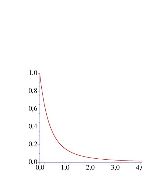
Figure 1: Variation of the time average $\overline{\eta}$ (see (37)) as a function of $\alpha$.

In particular, the expectation value of $J_{z}$ is given by $\langle J_{z}\rangle(t)=\eta(t)\langle J_{z}\rangle(0)$ with:

$$\eta(t)=\,\sqrt{\frac{2}{\pi}}\int_{-\infty}^{+\infty}\,\frac{{\rm e}^{-2\xi^{2}}}{\alpha^{2}+\xi^{2}}\left(\xi^{2}+\alpha^{2}\cos\sqrt{\alpha^{2}+\xi^{2}}\,\frac{\omega t}{\alpha}\right)\,{\rm d}\xi\enspace$$ (36)

(note that, with our definitions, $\frac{\omega t}{\alpha}=\frac{vt}{\sigma}$). $\eta(t)$ (obviously bounded by $\pm 1$) is clearly an oscillating function of time. This expression allows to discuss the unexpected behaviour of the average value of $J_{z}$ when $\alpha$ varies. First, let us look at the time-average value of $\eta$, $\overline{\eta}\equiv\lim_{t\rightarrow+\infty}\frac{1}{t}\int_{0}^{t}\eta(t^{\prime}){\rm d}t^{\prime}$. One readily finds:

$$\overline{\eta}=1-\sqrt{2\pi}\,\alpha\,{\rm e}^{2\alpha^{2}}[1-\Phi(\sqrt{2}\alpha)]\enspace$$ (37)

where $\Phi$ is the probability integral gradryz . $\overline{\eta}$ has the following behaviours:

$$\overline{\eta}\,\simeq\,\left\{\begin{array}[]{ll}1-\sqrt{2\pi}\,\alpha&\mbox{\quad$\alpha\ll 1$}\\ \frac{1}{4\alpha^{2}}&\mbox{\quad$\alpha\gg 1$}\end{array}\right.$$ (38)

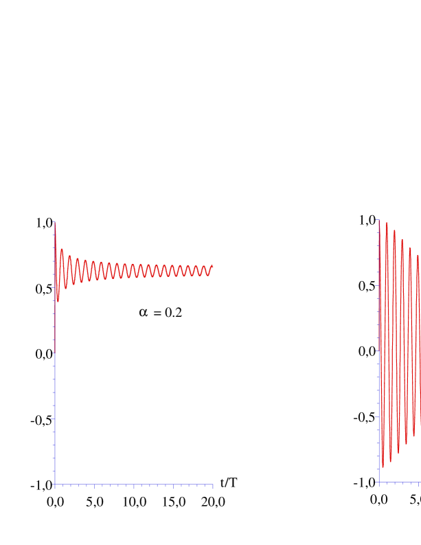
Figure 2: Variation in time of $\eta(t)$ for a narrow initial wave packet (left) and for a large one (right). For an infinitely narrow wave packet, $\langle J_{z}\rangle$ remains constant. The unit of time is one period $T$ of the Larmor precession.

In addition, it is readily seen that $1-2\overline{\eta}\leq\eta(t)\leq 1$. Thus, for $\alpha$ small, $\eta(t)$ oscillates around a value which is quite close to one, showing that $\langle J_{z}\rangle$ becomes nearly constant in time. On the contrary, for $\alpha$ large, the oscillation takes place symmetrically around a quite small value. The variation of $\overline{\eta}$ as a function of $\alpha$ is given in Fig. 1.

At short times, one has $\eta(t)\simeq 1-\frac{1}{2}(\omega t)^{2}$. The behaviour of $\eta(t)$ at large times is easily found by using a saddle-point method. We find:

$$\eta(t)\simeq\overline{\eta}+\frac{2\alpha}{\sqrt{\omega t}}\,\cos\left(\omega t+\frac{\pi}{4}\right)\enspace,\quad t\gg\mbox{min }(\frac{\sigma}{v},\,\omega^{-1})\enspace.$$ (39)

The enveloppe of the oscillation around the time averaged value $\overline{\eta}$ thus decreases as $t^{-1/2}$. The variation of $\eta(t)$ at any time is plotted in Fig.2 for two values of $\alpha$.

These results confirm the confinement-locking of the spin: whereas $J_{z}$ is not a constant of motion, narrowing the width of the initial wave packet yields an expectation value which is less and less varying in time.

From (33), the average position of the particle is easily calculated and can be written as:

$$\langle x\rangle(t)=Mvt\left[\overline{\eta}+\frac{\alpha^{3}}{\omega t}\sqrt{\frac{2}{\pi}}\int_{-\infty}^{+\infty}\frac{{\rm e}^{-2\xi^{2}}}{(\alpha^{2}+\xi^{2})^{3/2}}\sin\sqrt{\alpha^{2}+\xi^{2}}\,\frac{\omega t}{\alpha}\,{\rm d}\xi\right]\enspace.$$ (40)

This represents a drift motion, with a damped-in-time ($\propto t^{-1}$) oscillation around the central position $Mvt\overline{\eta}$, imaging the forward/backward motion of the particle within its wavepacket as the spin precesses, causing inversion of the velocity.

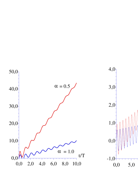
Figure 3: Variation in time of $\langle x\rangle(t)$ for four values of $\alpha$, when the initial state is an eigenvector of $J_{z}$. Note the different horizontal and vertical scales.

It is readily seen that $\langle x\rangle(t)$ is bounded for any time and any $\alpha$; one finds:

$$Mvt[\overline{\eta}-(\omega t)^{-1}]<\langle x\rangle(t)<Mvt[\overline{\eta}+(\omega t)^{-1}]\enspace.$$ (41)

This shows that, for such a preparation, the motion is always ballistic and simply approaches $\langle x\rangle(t)\simeq M\overline{\eta}vt$ at times which are large compared to the precession time scale. However, note that the effective velocity $\overline{\eta}v$ decreases rapidly when $\alpha$ becomes large (see (38) and Fig. 3). In the asymptotic regime, one precisely has:

$$\langle x\rangle(t)\simeq Mvt\left[\overline{\eta}+\frac{2\alpha}{(\omega t)^{3/2}}\sin\left(\omega t+\frac{\pi}{4}\right)\right]\enspace.$$ (42)

Note that in the limit $\alpha\rightarrow\,0$ but for an arbitrary initial spin state, one has $\langle J_{z}\rangle(t)=\,\langle J_{z}\rangle(0)$ and:

$$\langle x\rangle(t)=vt\hbar^{-1}\langle J_{z}\rangle(0)\enspace,\qquad\Delta x^{2}(t)=v^{2}t^{2}\hbar^{-2}\Delta J_{z}^{2}(0)\enspace,$$ (43)

in agreement with (24). The $\propto t^{2}$ increase of the mean-square dispersion merely reflects the fact that in this limit, the density is just the superposition of the $2J+1$ $\delta(x-Mvt)$ functions.

Obviously, the mean square deviation gives a first feeling about the spatial density, but the qualitative discussion given above convinces one that a given $t^{2}$ increase of $\Delta x^{2}(t)$ can be realized in a variety of ways, ranging from two moving sharp peaks to a gaussian-like flattening in situ. Clearly, a more precise analysis of the profile is required, and this is done in the following section for the $J=\frac{1}{2}$ case.

V Time evolution of the spatial density in the spin $\frac{1}{2}$ case

In the $J=\frac{1}{2}$ case, the evolution operator can be easily written explicitely. After some algebra, we find the propagator $U(p,\,t)$ as the following:

$$U(p,\,t)=\cos\frac{\Omega(p)t}{2}{\bf 1}-{\rm i}\sin\frac{\Omega(p)t}{2}\,\cos\theta(p)\,\sigma_{z}-{\rm i}\sin\frac{\Omega(p)t}{2}\,\sin\theta(p)\,\sigma_{y}\enspace$$ (44)

where the $\sigma_{u}$’s are the Pauli matrices. From this, one readily obtains the amplitudes $\psi_{\pm}(x,\,t)$, given by:

$$\psi_{\pm}(x,\,t)\,=\,\frac{1}{\sqrt{2\pi\hbar}}\int_{-\infty}^{+\infty}{\rm d}p\,{\rm e}^{\frac{{\rm i}}{\hbar}px}$$

$$\times\left[\left(\cos\frac{\Omega(p)t}{2}\mp{\rm i}\cos\theta(p)\sin\frac{\Omega(p)t}{2}\right)\,c_{\pm}\mp\sin\theta(p)\sin\frac{\Omega(p)t}{2}\,c_{\mp}\right]\,\phi(p)$$ (45)

Close inspection of the integrals in (45) again reveals that for any initial state which is even and real, the density $P(x,\,t)=\sum_{\varepsilon=\pm}|\psi_{\varepsilon}(x,\,t)|^{2}$ is even only when $|c_{+}|^{2}=|c_{-}|^{2}$ and $\frac{c_{+}}{c_{-}}$ purely imaginary, i. e. when the initial spin state is an eigenvector of $J_{y}$. In all other cases, $P(-x,\,t)\neq P(x,\,t)$.

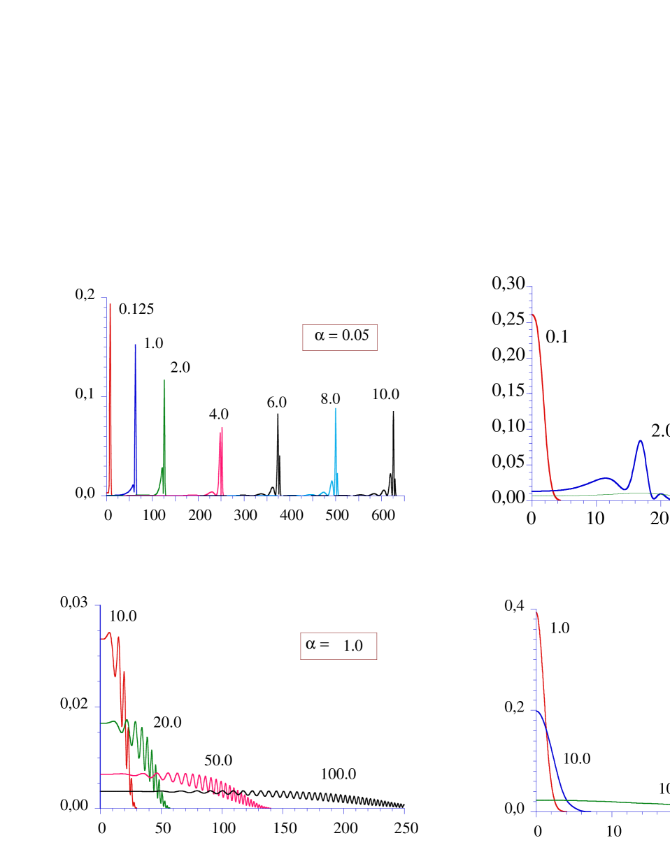
Figure 4: Snapshots of the (symmetric) density profile at successive times $t$ for various values of the parameter $\alpha$; each curve is labelled by $\frac{t}{T}$ where $T$ is the Larmor period $\frac{2\pi}{\omega}$. The abscissa unit is the width $\sigma$ of the initial gaussian packet. Note the different scales from one drawing to another.

In the following, we restrict to the symmetric case, taking $c_{+}=\frac{1}{\sqrt{2}}$ and $c_{-}=\frac{{\rm i}}{\sqrt{2}}$, corresponding to $|\chi\rangle\,=\,|+\rangle_{y}$. Then, the density can be written as follows:

$$P(x,\,t)\,=\,\frac{1}{\sqrt{2\pi}\sigma}\sum_{r=1,\,2,\,3}|I_{r}(x,\,t)|^{2}\enspace,$$ (46)

where the three quantities $I_{r}$ are given integrals. With the gaussian wave packet (18), the latter explicitely write ($X=\frac{x}{\sigma}$):

$$I_{1}(x,\,t)\,=\,\frac{\alpha}{\sqrt{\pi}}\int_{-\infty}^{+\infty}{\rm d}\xi\,\frac{{\rm e}^{-\xi^{2}+{\rm i}\xi X}}{\sqrt{\alpha^{2}+\xi^{2}}}\,\sin\sqrt{\alpha^{2}+\xi^{2}}\frac{vt}{2\sigma}\enspace,$$ (47)

$$I_{2}(x,\,t)\,=\,\frac{1}{\sqrt{\pi}}\int_{-\infty}^{+\infty}{\rm d}\xi\,{\rm e}^{-\xi^{2}+{\rm i}\xi X}\,\frac{\xi}{\sqrt{\alpha^{2}+\xi^{2}}}\,\sin\sqrt{\alpha^{2}+\xi^{2}}\frac{vt}{2\sigma}\enspace,$$ (48)

$$I_{3}(x,\,t)\,=\,\frac{1}{\sqrt{\pi}}\int_{-\infty}^{+\infty}{\rm d}\xi\,{\rm e}^{-\xi^{2}+{\rm i}\xi X}\,\cos\sqrt{\alpha^{2}+\xi^{2}}\frac{vt}{2\sigma}\enspace.$$ (49)

These expressions allow an easy numerical calculation of the density $P(x,\,t)$ in various cases; the results are shown in Fig. 4 and display the extreme variety of $P(x,\,t)$ when the single parameter $\alpha$ varies. For $\alpha$ small (remember this corresponds to QRW), the (two) peaks structure is clearly visible, and displays small satellites at the back of the packet. They are easily understood as arising from a (quantum) path in which the particle has undergone a small number of precessions. This is confirmed by the $\alpha=\frac{1}{3}$ curves: it can be checked that the number of peaks is close to $\frac{t}{T}$, where $T$ is the Larmor period. The extreme-right peak arises when the particle did not precess at all, then comes a secondary peak associated with one precession, and so on. When $\alpha$ increases, the structure is still present but diminishes quickly as time goes on. Eventually, for $\alpha$ large enough, the profile does not display any structure and vaguely looks like a standing gaussian wave packet. As a whole, the profile is rather sensitive to $\alpha$; also note that $P(x,\,t)$ remains notably non-zero in the central region even at large times (see below, especially (52)).

Approximate analytical expressions of the density can also be obtained (see Appendix). For $\alpha\ll 1$, we find that:

$$P(x,\,t)\,\simeq\,\frac{\alpha^{2}}{16(2\pi)^{3/2}}\left|\int_{-\infty}^{+\infty}\,{\rm d}X^{\prime}\,{\rm e}^{-\frac{1}{4}(X-X^{\prime}-\frac{vt}{2})^{2}}H^{(2)}_{1}(\tilde{X}^{\prime})\right|^{2}\enspace$$ (50)

where $\tilde{X}^{\prime}=\alpha\sqrt{\frac{vt}{\sigma}|X^{\prime}|}$ and where $H^{(2)}_{1}$ is the conventional Hankel function. Details given in the Appendix allow to understand that in this case ($\alpha\ll 1$), the two main peaks moving with the velocity $\frac{v}{2}$ are accompanied by small satellites, corresponding to those quantum paths with a few precessions.

On the other side, for $\alpha\gg 1$, one finds the plain gaussian distribution:

$$P(x,\,t)\,\simeq\,\frac{1}{\sqrt{2\pi}\Delta(t)}{\rm e}^{-\frac{x^{2}}{2\Delta(t)^{2}}}\enspace,\qquad\Delta\,=\,\sigma\,\left[1+\left(\frac{v^{2}t}{4\sigma^{2}\omega}\right)^{2}\right]^{1/2}\enspace.$$ (51)

Because the precession is rapid, the particle does not move in the mean, but the effect is not averaged to zero and produces a linear in time increase of the width of the distribution.

Generally speaking, it appears that, for any $\alpha$, the central region remains populated due to the fact that $P(x=0,\,t)$ decreases rather slowly in time. Indeed, a stationnary-phase argument shows that:

$$P(x=0,\,t)\,\simeq\,\frac{1}{\sqrt{2\pi}\Delta(t)}\,\sim t^{-1}\quad\,\forall\,t\gg\mbox{Max }\left(\frac{2\pi}{\omega},\,\frac{\sigma}{v}\right)\enspace.$$ (52)

As for any initial state, the mean square dispersion of the coordinate always increases $\propto t$ at large times, and can be readily calculated for the symmetric case, using the results of section IV. In particular, one finds:

$$\lim_{t\rightarrow+\infty}\frac{\Delta x(t)}{t}\,=\,\frac{1}{2}\langle\cos^{4}\theta\rangle^{1/2}\,v\,\equiv\,V(\alpha)\,v\enspace.$$ (53)

with:

$$\langle\cos^{4}\theta\rangle\,=\,1+\alpha^{2}-\sqrt{2\pi}\,\alpha(3+4\alpha^{2}){\rm e}^{2\alpha^{2}}\,[1-\Phi(\sqrt{2}\alpha)]\enspace.$$ (54)

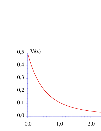
Figure 5: Variation as a function of $\alpha$ of the velocity $V$ of the standard deviation $\Delta x(t)$ (see (55)).

$V(\alpha)$ is a monotonically decreasing function of $\alpha$ (see Fig. 5), with the following behaviours:

$$V(\alpha)\,\simeq\,\left\{\begin{array}[]{ll}\frac{1}{2}\left(1-3\sqrt{\frac{\pi}{2}}\,\alpha^{2}\right)&\mbox{\quad$\alpha\ll 1$}\\ \frac{\sqrt{3}}{8\alpha^{2}}&\mbox{\quad$\alpha\gg 1$}\end{array}\right.$$ (55)

This means that, apart from small damped in time oscillations, the motion is essentially ballistic, with a velocity $V(\alpha)$ going to zero when the precession frequency increases. With the reduced units used in Fig.4, the width of the distribution is $2\pi/(\alpha V(\alpha))\,(t/T)$; rough estimates show that the gross features of the density profile are in agreement with the latter expression for the standard deviation.

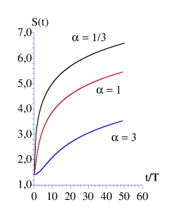
Figure 6: Variation in time of the Shannon entropy $S(t)$ (left). The right part shows the ratio $S(t)/\ln t$, which becomes a constant at large times.

As a final measure of the profile, let us analyse the Shannon entropy, defined as:

$$S(t)\,=\,-\int_{-\infty}^{+\infty}{\rm d}x\,P(x,\,t)\ln P(x,\,t)\enspace.$$ (56)

Three typical plots are given in the left part of Fig. 6, showing that $S(t)$ – an ever-increasing function in time –, changes gently with $\alpha$ and does not display a transition reflecting the bimodal/unimodal cross-over. In addition, it is seen that $S(t)\propto\ln\,t$ at large times, which means that, as it is often the case, $S(t)\propto\ln\Delta x(t)$.

VI Conclusions

In this paper, we presented a simple model describing the dynamics of a particle with a linear dispersion law, when the direction of motion is determined by the value of the spin, the former being able to flip due to magnetic impurity scatttering or by coupling with an external field. The resulting intrication between orbital and spin degrees of freedom yields a rather rich and complex dynamics with unexpected features, governed by the single parameter $\alpha=\sigma\omega/v$ measuring the ratio between the time of flight and the Larmor period $T$.

The most surprising fact is spin-freezing when the width of the initial wave packet becomes quite small: narrowing the latter produces stronger and stronger shielding of the spin which can thus keep for ever the memory of its initial value. This robustness could be of interest in applications where the spin value carries sensitive information, e. g. in spintronics and in quantum spin computation.

Aside this remarkable fact, the density profile itself shows up a variety of shapes which reflect the competition between motion in space and Larmor precession. In the intermediate case where the characteristic time of flight $\sigma/v$ is of the order of the precession period, the profile displays a rich structure corresponding to the various quantum paths with zero, one, two,…  precessions: the number of rotations can be directly read by looking at the maxima of the density. In one extreme case ($\alpha\ll 1$), one recovers conventional Quantum Random Walk in a space-time continuous framework, and its characteristic multimodal (bimodal for $J=1/2$) distribution. In the opposite case $\alpha\gg 1$, the particule hardly moves in the mean because of rapid precession, but the width of the packet increases proportionally to the time $t$.

Another interesting fact, already discussed in the past in the restricted QRW limit, is the role of the phases present in the initial spin state: it turns out that the space-density is even only when the initial state is an eigenvalue of the transverse spin $J_{y}$, i. e. when the coefficients have the same modulus and a definite phase relationship. For an infinitely narrow wave packet, this specific property disappears, and the subsequent motion becomes phase-independent: we do not have a simple explanation of this phase symmetry breaking.

In all cases, the RMS deviation of the coordinate $\Delta x(t)$ increases like $t$, much faster than in classical random motion. This universal increase integrates in fact various shapes, from sharp rapidly moving well defined peaks, to a standing flattening gaussian distribution. The same can be said about the Shannon entropy, which does not show up any cross-over when $\alpha$ varies; it essentially behaves like $\ln\Delta x$, as is often the case, and thus increases $\propto\,t$ at times large enough.

Some of our results are restricted to the $J=1/2$ case. Obviously enough, generalization to arbitrary $J$ is appealing; in particular, it would be interesting to look at the high-$J$ (quasi-classical limit), especially in order to analyse the above mentionned phase symmetry-breaking phenomenon. Furthermore, it would be interesting to check whether the above shielding effect is robust against phase decoherence, i. e. to develop simple models incorporating coupling to a quantum or classical bath. Work in these directions is in progress.

Appendix

We now briefly sketch the methods allowing to obtain the approximate expressions (50) and (51) given in the main text. In all cases, the approximations start with the expression of the time-evolution operator $U$, and preserve unitarity.

Let us begin with the easiest case, namely $\alpha\gg 1$, i. e. when the spin precesses quickly and when the drift is slow. Then, the angle $\theta$ in (21) is close to $\frac{\pi}{2}$. From (45), one readily obtains:

$$\psi_{+}(x,\,t)\,\simeq\,\frac{1}{(2\pi)^{3/4}\sigma^{1/2}}\int_{-\infty}^{+\infty}\,{\rm d}k\,{\rm e}^{-k^{2}+{\rm i}kX}\,{\rm e}^{-{\rm i}\omega t\sqrt{1+(k/\alpha)^{2}}/2}\enspace,$$ (57)

and $\psi_{-}(x,\,t)={\rm i}\,\psi_{+}(-x,\,t)$. Taking advantage of the gaussian cut-off, the square-root can be safely expanded when $\frac{k}{\alpha}\sim\frac{1}{\alpha}\ll 1$; the resulting gaussian integrals are readily evaluated, and one eventually finds the result given in (51).

The other case, $\alpha\ll 1$, (swift drift ans slow precession) is much more involved, due to the fact that the limit $\alpha\rightarrow\,0$ is highly singular. From (21), the expression of $\psi_{+}$ is:

$$\psi_{+}(x,\,t)\,=\,\frac{1}{(2\pi)^{3/4}\sigma^{1/2}}\int_{-\infty}^{+\infty}\,{\rm d}k\,{\rm e}^{-k^{2}+{\rm i}kX}\,{\rm e}^{-{\rm i}\frac{vt}{2\sigma}\,\sqrt{k^{2}+\alpha^{2}}}\enspace,$$ (58)

and one still has $|\psi_{-}(x,\,t)|=|\psi_{+}(-x,\,t)|$. No simple approximation seems possible on such an expression but, since one expects that the rapidly moving peak aroud $x\sim\frac{vt}{2}$ be slighthy modulated by the precession, it is tempting to write an approximation using a convolution integal. For that purpose, we rewrite (58) as follows:

$$\psi_{+}(x,\,t)\,=\,\frac{1}{(2\pi)^{3/4}\sigma^{1/2}}\int_{-\infty}^{+\infty}\,{\rm d}k\,{\rm e}^{{\rm i}kX}\,{\rm e}^{-k^{2}-{\rm i}k\frac{vt}{2\sigma}}\,{\rm e}^{{\rm i}\frac{vt}{2\sigma}\,(k-\sqrt{k^{2}+\alpha^{2}})}\enspace.$$ (59)

By the convolution theorem, this means that $\psi_{+}$ can be expressed as:

$$\psi_{+}(x,\,t)\,=\,\frac{1}{2^{3/4}\pi^{1/4}\sigma^{1/2}}\int_{-\infty}^{+\infty}\,{\rm d}X^{\prime}\,{\rm e}^{-\frac{1}{4}\left(X-X^{\prime}-\frac{vt}{2\sigma}\right)^{2}}F(X^{\prime},\,t)\enspace,$$ (60)

where $F(X,\,t)$ is the Fourier transform:

$$F(X,\,t)\,=\,\frac{1}{2\pi}\int_{-\infty}^{+\infty}\,{\rm d}k\,{\rm e}^{{\rm i}kX}\,{\rm e}^{{\rm i}\frac{vt}{2\sigma}\,(k-\sqrt{k^{2}+\alpha^{2}})}\enspace.$$ (61)

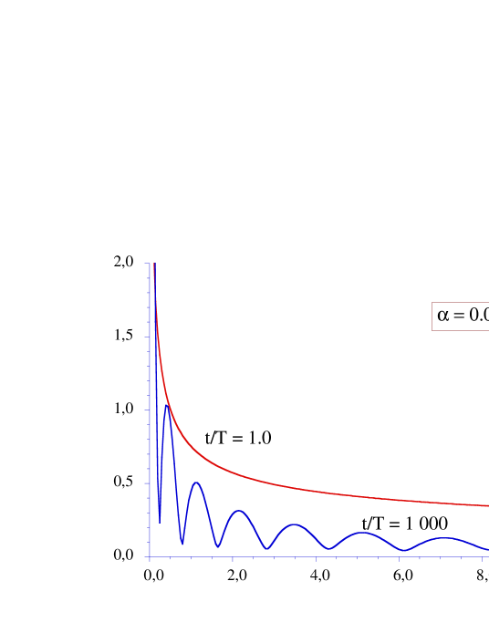
Figure 7: Kernel $F(X,\,t)$ defined in (62) for the convolution (see (60)).

Note that for $\alpha=0$, $F(X)$ reduces to the Dirac function $\delta(X)$. Now, we expand the (small) phase factor as $k-\sqrt{k^{2}+\alpha^{2}}\simeq k-|k|(1+\frac{\alpha^{2}}{2k^{2}})$, allowing to write:

$$F(X,\,t)\,\simeq\,f(X,\,t)-f(X+\frac{vt}{2\sigma},\,t)\enspace$$ (62)

where the function $f$ is defined as:

$$f(X,\,t)\,=\,\frac{1}{2\pi}\int_{0}^{+\infty}\,{\rm d}k\,{\rm e}^{{\rm i}X[k-\alpha^{2}vt/(4\sigma Xk)]}\enspace.$$ (63)

This function can be expressed with the Hankel functions $H^{(1,2)}_{\nu}(z)$ gradryz . A somewhat tedious calculation yields:

$$f(X,\,t)\,=\,\frac{\alpha}{4}\mbox{sgn}(X)\sqrt{\frac{vt}{\sigma|X|}}\,H^{(2)}_{1}\left(\alpha\sqrt{\frac{vt}{\sigma}|X|}\right)\enspace.$$ (64)

By (62), this completes the determination of the kernel $F(X,\,t)$; nevertheless, analysis reveals that the second term in (62) is quickly negligible, because of the rapid translation of each well-defined peak, so that one nearly always has $F(X,\,t)\,\simeq\,f(X,\,t)$. Fig. 7 shows the variation of $|F(X,\,t)|$ as a function of the reduced abscissa $X=\frac{x}{\sigma}$, at short and long times. In all cases, the strong peak in $F(X,\,t)$ near $X=0$ explains the persistence of the two main peaks in the density $P(x,\,t)$, whereas slowly decreasing ($\sim X^{-1/2}$) oscillations are responsible for the secondary small peaks located just behind the main one. The minima arise from the zeroes of the $Y_{1}$ Bessel function included in $H^{(2)}_{1}$, which becomes denser and denser as time goes on; this can explain that at large times, the moving peaks for $\alpha\ll 1$ eventually grows up (see Fig. 4, upper left).

I am indebted to C. Caroli, R. Mosseri, P. Ribeiro and J. Vidal for helpful and numerous fruitful discussions.

References

References

- (1) Y. Aharonov, L. Davidovich, Quantum Random Walks, Phys. Rev. A. 48, 1687 (1993)
- (2) A. J. Leggett, S. Chakravarty, A. T. Dorsey, M. P. A. Fisher, A. Garg, W. Zwerger, Dynamics of the disipative two-state system, Rev. Mod. Phys., 59, 1 (1987)
- (3) Cl. Aslangul, N. Pottier, D. Saint-James, Time-behaviour of the correlation functions in a simple dissipative quantum model, J. Stat. Phys., 40, 167 (1985)
- (4) A. Ambainis, E. Bach, A. Nayak, A. Vishwanath and J. Watrous, One-dimensional quantum walks, Proc. 33rd Ann. Symp. on Theory of Computing, p. 37 (New York, ACM, 2001)
- (5) A. Nayak and A. Vishwanath Briegel, Quantum walk on the line, quant-ph/0010117
- (6) W. Dür, R. Raussendorf, V. M. Kendon and H.-J. Briegel, Quantum random walks in optical lattices, quant-ph/0207137
- (7) J. Kempe, Quantum random walks – an introductory overview, quant-ph/0303081
- (8) C.W. Gardiner, Handbook of Stochastic Methods (Springer, 1990)
- (9) Ph. Blanchard and M.-O. Hongler, Quantum Random Walks and Piecewise Deterministic Evolutions, Phys. Rev. Let., 92, 120601 (2004)
- (10) B. Misra and E.C.G. Sudarshan, The Zeno’s paradox in quantum theory, J. Math. Phys., 18, 756 (1977)
- (11) W.M. Itano, D.H. Heinzen, J.J. Bolllinger and D.J. Wineland, Quantum Zeno effect, Phys. Rev., A41, 2295 (1990)
- (12) J. Kempe, Quantum Random Walk Hits Exponentially Faster, quant-ph/0205083
- (13) J.M. Luttinger, An exactly soluble model of a many-fermion system, J. Math. Phys., 9, 1154 (1963)
- (14) I.D. Vagner, Nuclear spintronics: quantum Hall and nano-objects, cond-mat/0403087
- (15) J.P. McGuire, C. Ciuti, and L.J. Sham, Theory of spin transport induced by ferromanetic proximity on a two-dimensional electron gas, Phys. Rev., B69, 115339 (2004)
- (16) C.-K. Yang, J. Zhao, and J. P. Lu, Magnetism of Transition-Metal/Carbon-Nanotube Hybrid Structures, Phys. Rev. Let., 90, 257203 (2003)
- (17) L.S. Levitov and E.I. Rashba, Dynamical spin-electric coupling in a quantum dot, Phys. Rev., B69, 115324 (2004)
- (18) M.I. Dyakonov, Spintronics?, cond-mat/0401369
- (19) P.G. de Gennes, Superconductivity of Metals and Alloys (Benjamin, New York, 1966)
- (20) H. Takayama, Y.R. Lin-Liu and K. Maki, Continuum model for solitons in polyacetylene, Phys. Rev., B21, 2388 (1980)
- (21) I. S. Gradshteyn and I. M. Ryzhik, Table of Integrals, Series and Products (Acad. Pr., New York, 1980)