On the classical-quantum correspondence for the scattering dwell time

Abstract

Using results from the theory of dynamical systems, we derive a general expression for the classical average scattering dwell time $\langle\tau\rangle$. Remarkably, $\langle\tau\rangle$ depends only on a ratio of phase space volumes. We further show that, for a wide class of systems, the average classical dwell time is not in correspondence with the energy average of the quantum Wigner time delay.

I Introduction

The study of the time a quantum collision process takes to occur is one of the most interesting chapters in scattering theory. This problem turns out to be subtle and fascinating due to the lack of a Hermitian operator to measure the time as a quantum observable. Hence, one inevitably has to rely on auxiliary constructions to quantify the time spent by a scattering process. To that end several ingenious strategies have been proposed over the past 50 years Carvalho02 . In a pioneering work, Eisenbud and Wigner Wigner55 proposed measuring the scattering delay time by recording the peak position of wave packets scattered in one-dimension. This simple construction, that just invokes the concept of group velocity, already captures the deep connection between the energy variations of the scattering phase shift and the delay time. In 1960, Smith Smith60 put forward an alternative scheme, applicable to stationary scattering processes, where the scattering dwell time is associated to the ratio between the probability of finding the particle inside the scattering region and the flux through its surface. This approach has the advantage of eliminating the necessity of wave-packets and can be easily generalized to multi-channel scattering. As a result, the dwell-time $\tau_{W}(E)$ is expressed as

$$\tau_{W}(E)=-\frac{i\hbar}{N}\sum_{a,b=1}^{N}{\sf S}_{ab}^{\ast}\frac{\partial{\sf S}_{ba}}{\partial E}~{},$$ (1)

where the scattering matrix ${\sf S}$, that encodes all accessible information about the scattering process, is taken at the energy $E$. The sums in (1) run over all $N$ open asymptotic scattering channels. The time $\tau_{W}(E)$ is usually called Wigner time delay.

Is $\tau_{W}(E)$ in correspondence with the classical dwell time for general scattering systems? To answer this question we approach the problem from the classical side. We use the theory of dynamical systems to obtain a remarkably simple and general expression for the classical dwell time, revealing its geometric nature. Comparing this result with the semiclassical limit for the energy averaged quantum dwell-time, we find that the quantum-classical correspondence does not hold in general.

The present analysis does not contradict a previous study of ours Lewenkopf04 . There we followed a different path, applicable only to chaotic systems, and concluded that the classical-quantum correspondence for the dwell time holds. Here, approaching the problem in a way that is insensitive to the details of the dynamics, we vastly expand Lewenkopf04 and show that the correspondence fails in the more general case of systems with mixed phase space.

The paper is organized as follows. In Sec. II we derive the central result of this paper, namely, a general expression for the classical average time delay in terms of the system phase space volume. It is key to our analysis the formulation of the scattering process as the first return of a measure-preserving map, allowing us to benefit from well-known results of ergodic theory. In Sec. III we discuss the semiclassical limit of the energy-averaged Wigner time delay. We conclude presenting, in Sec. IV, a comparison between the classical and quantum dwell time. We show that, in general, these two quantities do not coincide.

II The classical dwell time

Poincaré sections are extremely useful tools for the analysis of phase space structures in bounded low-dimensional Hamiltonian systems: These surfaces of section allow us to reduce the continuous time evolution of dynamical systems to discrete mappings, much simpler to work with.

Surfaces of section are essential for the proper definition of a scattering problem. Consider the scattering of a particle by a potential. The description of the scattering process requires two control surfaces for detecting the state of the particle before and after the scattering event. The description of all possible scattering processes demands the control surfaces to be chosen so as to enclose the scatterer completely. In this case we can consider just one surface for registering both the states of incoming and outgoing particles.

Let us illustrate these concepts by discussing a generic scattering process in three-dimensions. We choose a spherical control surface enclosing the region where the potential is non-negligible. A point on the associated Poincaré surface $\Sigma$ has coordinates $({\bf q},{\bf p}_{\|})$, where $\bf q$ represents a position on the sphere and ${\bf p}_{\|}$ the conjugate (angular) momentum. An incoming state is completely specified by giving its coordinates on $\Sigma$ together with the condition that the momentum normal to the sphere, ${\bf p}_{\perp}$, must point inwards (the modulus of ${\bf p}_{\perp}$ is fixed by energy conservation). The incoming state then evolves inside the scattering region, along a trajectory given by Hamilton equations. It eventually intersects $\Sigma$ again at the exit point $({\bf q}^{\prime},{\bf p}_{\|}^{\prime})$ and escapes. Hence, any scattering process can be essentially viewed as the first return map of $\Sigma$ Ozorio00 ,

$${\cal S}:\Sigma\mapsto\Sigma\;,\qquad({\bf q},{\bf p}_{\|})\stackrel{{\scriptstyle\cal S}}{{\longmapsto}}({\bf q}^{\prime},{\bf p}_{\|}^{\prime})\;.$$ (2)

As a consequence of the Poincaré-Cartan theorem, this map is volume-preserving Ozorio88 .

The structure of the classical scattering problem has a clear quantum mechanical counterpart. The quantum analogue of the classical Poincaré surface is the Hilbert space ${\cal H}_{\Sigma}$ associated to $\Sigma$. The quantum scattering ${\sf S}$-matrix is a linear operator of ${\cal H}_{\Sigma}$, mapping incoming states into outgoings ones. The Poincaré map (2) is the classical limit of ${\sf S}$. Conversely, the scattering matrix ${\sf S}$ can be thought of as the quantization of ${\cal S}$ Rouvinez95 . The unitarity of ${\sf S}$ is the quantum counterpart of the classical volume conservation Miller74 ; Smilansky91 .

This parallel between classical and quantum scattering processes serves to facilitate the determination of some quantum-classical correspondences. For instance, and very useful for what follows, it becomes clear that the classical analogue of an average over “channels” (a complete basis set of ${\cal H}_{\Sigma}$) is an average over $\Sigma$ weighted by its Liouville measure.

Let us now discuss in detail a very simple scattering system: a two-dimensional billiard with an attached pipe. The case of a smooth cavity with several (smooth) pipes in two or three dimensions, or even, the scattering of asymptotically free particles by a smooth potential, are conceptually equivalent to the two-dimensional billiard with a single pipe, and will be discussed later.

The physical process we analyze is: A classical particle propagates along the pipe and eventually arrives at the billiard, where it elastically bounces $n$ times at the walls before escaping (see Figure 1). A Poincaré section $\Sigma$, transverse to the pipe, separates the scattering region (interior, billiard region, interaction region) from the asymptotic region (exterior, pipe). We ask the average number of times $\langle n\rangle$ a particle bounces before escaping, or, what is the average dwell time $\langle\tau\rangle$ of a particle inside the billiard. As already mentioned, the appropriate measure for averaging gives equal weights to all points on $\Sigma$ having the same energy $E$.

In what follows we show that the answers to these questions are given by very simple ratios between phase space volumes. Then we argue that our results are also applicable to more general geometries.

II.1 Birkhoff maps

Let us consider the Birkhoff section taken along the billiard walls, see Fig. 1.

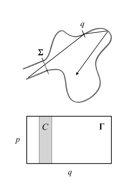
Figure 1: (top) Billiard with attached pipe. The Poincaré section $\Sigma$ (dashed line) defines an auxiliary closed billiard. (bottom) Boundary phase space $\Gamma$ of the scattering billiard. The phase space coordinates are $q$, the position along the boundary, and $p$, its conjugate momentum. The shaded rectangle $C$ corresponds to the closure $\Sigma$.

The coordinates $(q,p)$, where $q$ is the particle position on the billiard boundary and $p$ is its conjugate momentum, entirely characterize the particle phase space $\Gamma$. The dynamics inside the scattering region is given by the Birkhoff (or boundary) map $T$ that propagates a particle between successive bounces, i.e., from a phase space point $(q,p)\in\Gamma$ to the one where the next bounce takes place.

Now we “close” the billiard by adding a straight segment normal to the pipe axis Ozorio00 . The Poincaré section associated to this segment, $\Sigma$, closes the Birkhoff section $\Gamma$. Thus, the scattering process can be identified with the first-recurrence map to $\Sigma$, now considered as a part of $\Gamma$; the dwell time becomes the first-return time to $\Sigma$. Figure 1 shows the boundary phase space $\Gamma$, namely, a rectangle of length equal to the perimeter of the closed billiard and height $2p_{\rm max}$, with $p_{\rm max}^{2}=2mE$, where $m$ is the particle mass and $E$ its energy. The shaded vertical strip corresponds to the closure $\Sigma$, and is denoted by $C$. The inclusion of more pipes to the billiard is accounted for by adding the corresponding (disjoint) vertical stripes. This construction can be easily extended to higher dimensions.

We recall that $n$ is the return time measured in units of bounces against the billiard walls. Its average is

$$\langle n\rangle=\frac{\sum_{n=1}^{\infty}n\,\mu(C_{n})}{\mu(C)}\;,$$ (3)

where $C_{n}\subset C$ is the subset of initial conditions that first return to $C$ after $n$ iterations of the boundary map $T$ and $\mu$ refers to the volume measure in $\Gamma$. Using measure-preservation arguments, it is not difficult to show that $\sum_{n=1}^{\infty}n\,\mu(C_{n})=\mu\left(\bigcup_{n=1}^{\infty}T^{n}C\right)$ Cornfeld82 . Hence, Eq. (3) becomes

$$\langle n\rangle=\frac{\mu\left(\bigcup_{n=1}^{\infty}T^{n}C\right)}{\mu(C)}\;,$$ (4)

which now expresses the time delay as a quotient of two measures: The denominator is the measure of the closure; the numerator represents the measure of the inner phase space that is explored by the ensemble of scattering trajectories. For an ergodic dynamics the set $\bigcup_{n=1}^{\infty}T^{n}C$ clearly coincides with the full phase space $\Gamma$. Remarkably, even nonergodic Birkhoff’s maps very often satisfy the weak ergodicity condition

$$\bigcup_{n=1}^{\infty}T^{n}C\equiv\Gamma^{\prime}=\Gamma\;.$$ (5)

For instance, it is simple to verify that the circle billiard Blumel92 ; Ozorio00 , an archetype of integrable dynamics, satisfies Eq. (5) for any straight closure $\Sigma$.

As a result, for weakly ergodic billiards we find that $\langle n\rangle={\mu(\Gamma)}/{\mu(C)}$. The weak-ergodicity condition is not verified by systems containing stable islands that cannot be reached from the outside, as for instance, the cosine-shaped billiard cosine . In these cases we replace $\Gamma$ by $\Gamma^{\prime}$, the phase space that is effectively explored by the scattering orbits to write

$$\langle n\rangle=\frac{\mu(\Gamma^{\prime})}{\mu(C)}\;.$$ (6)

The expression above shows that for both ergodic and non-ergodic systems $\langle n\rangle$ is finite. Thus, the probability of first returning after $n$ iterations,

$$P(n)=\frac{\mu(C_{n})}{\mu(C)}\;,$$ (7)

must decay faster than $1/n^{2}$. In some cases numerical simulations may suggest a divergent average return time. Note, however, that the true asymptotic decay may settle only after very long times Chirikov99 .

II.2 Continuous time

The real, continuous, time-delay problem is addressed in analogy to the simple one presented above. To make a link between continuous dynamics and maps we invoke the stroboscopic map $T_{\Delta t}$, i.e., a discretization of the continuous evolution into time steps of length $\Delta t$. The continuum limit is obtained by making $\Delta t\to 0$. The map $T_{\Delta t}$ acts on the full phase space of the scattering system, namely, a four-dimensional space for a planar billiard.

In order to adapt Eq. (6) to the present context, we note that the set of incoming states $C$ has zero measure when thought of as a subset of the full phase space: It has to be substituted by a properly defined set having finite measure, which we call $\overline{C}$. The simplest way of choosing $\overline{C}$ is by letting $C$ acquire two extra dimensions: in the direction normal to the energy surface, and in the direction parallel to the phase space flow. The corresponding additional canonical coordinates are the energy $E$ and the time $t$ measured along the trajectories starting at the section $\Sigma$. The variables $E$ and $t$, together with the coordinates on $\Sigma$, form a local canonical set. When $C$ grows in “thicknesses” by $\Delta E$ and $\Delta t$, we have the simple relation between measures

$$\mu(\overline{C})=\mu(C)\,\Delta E\,\Delta t\;.$$ (8)

The dwell time is then given by Balakrishnan00

$$\langle\tau\rangle=\lim_{\Delta t\to 0}\Delta t\,\frac{\mu(\overline{\Gamma^{\prime}})}{\mu(\overline{C})}\;,$$ (9)

where

$$\overline{\Gamma^{\prime}}=\bigcup_{n=1}^{\infty}(T_{\Delta t})^{n}\overline{C}\;.$$ (10)

The quantity $\overline{\Gamma^{\prime}}$ represents the inner phase space for the continuous dynamics that can be accessed from outside. It has an energy thickness $\Delta E$.

By construction, the set $\overline{C}$ has the important property that all its points enter the scattering region after one time step $\Delta t$, namely,

$$\mu(\overline{C}\cap T_{\Delta t}\overline{C})=0\;.$$ (11)

This avoids the problem of having to subtract spurious contributions to the dwell time arising from non-scattering orbits Balakrishnan00 .

Let us now express Eq. (9) in terms of more appealing quantities. Define $\Omega$ to be the phase space volume contained by the energy shell $E$ within the scattering region (as before, primes will indicate “accessible from outside”). Then

$$\mu(\overline{\Gamma^{\prime}})=\frac{\partial\Omega^{\prime}}{\partial E}\Delta E\;.$$ (12)

We recall that $\mu(C)$ is the phase space volume contained by the energy shell $E$ within the section $\Sigma$. We now switch to a more standard notation and, from now on, we call it $\Omega_{\Sigma}$. Gathering everything and substituting into Eq. (9) we arrive at

$$\langle\tau\rangle=\frac{1}{\Omega_{\Sigma}}\frac{\partial\Omega^{\prime}}{\partial E}\;.$$ (13)

This remarkable formula is exact and holds irrespective of the dynamics being chaotic, regular or mixed. After making the proper identifications, Eq. (13) can also be applied to billiard systems in three (or higher) dimensions.

For the sake of illustration, let us, for instance, use Eq. (13) to calculate the mean time between collisions for a closed billiard. In this case, we have to choose $\Sigma$ as the phase space corresponding to the full boundary $\cal{L}$. The weak ergodicity condition is obviously satisfied and the average bounce time reads $\tau_{\rm b}=(\partial\Omega/\partial E)/\Omega_{\cal{L}}$ for any billiard, truly ergodic or not. For the two-dimensional case, $\Omega_{\cal{L}}=2mv{\cal L}$ and $\Omega=\pi p^{2}{\cal A}=2\pi mE{\cal A}$ ($v$ = velocity, ${\cal L}$ = perimeter, ${\cal A}$ = area). Then we arrive at the well-known result $\tau_{\rm b}=\pi{\cal A}/v{\cal L}$, as heuristically shown in Ref. Jarzynski93 and proven in Ref. Chernov97 .

II.3 Smooth systems

The extension of our findings to smooth systems is immediate. The boundary that so far defined the system billiard-plus-pipe now is thought as the level curve of a smooth potential. The motion in the waveguide is free in the longitudinal direction ($\hat{x}$). In the directions transverse to the waveguide ($\hat{y}$) the dynamics is governed by a smooth Hamiltonian $H_{\perp}(y,p_{y})$.

The analysis of Sec. II.2 applies equally well to this case Thus, the formula for the dwell time is also Eq. (13), with the following definitions. $\Omega_{\Sigma}$ is the measure of the phase space in the Poincaré section lying inside the energy shell $H_{\perp}=E$,

$$\Omega_{\Sigma}=\int_{H_{\perp}\leq E}dy\,dp_{y}\;.$$ (14)

$\Omega$ is the volume of the inner phase space with energy less than $E$. Assuming that the scatterer lies in the region $x>0$, we have

$$\Omega=\int_{H\leq E\;\;{\rm and}\;\;x>0}dx\,dy\,dp_{x}\,dp_{y}\;.$$ (15)

The case of a particle scattered off a smooth potential in three dimensions can be accounted for by enclosing the scatterer with a large enough spherical shell (the Poincaré section $\Sigma$). Then one defines the delay time as the (average) return time to $\Sigma$ minus the return time when there is no potential. Both return times are special instances of Eq. (13), the free-flight time being just the average bounce time of a spherical billiard.

III Average Wigner time-delay

The Wigner time delay $\tau_{W}(E)$, given by Eq. (1), fluctuates as a function of the energy. Large time delays are due to resonant scattering, whereas off-resonance scattering corresponds to direct processes that spend short times in the interaction region. This picture becomes particularly clear in the regime of isolated resonances: Long time delays occur at narrow energy windows around each resonance, in the remaining energy interval scattering processes are fast (direct). The important energy scale that emerges from this picture is the mean resonance spacing. When the resonances are overlapping, the separation of time scales is less clear, and fluctuations are much smaller Lewenkopf91 .

By averaging the Wigner time delay over an energy window $\Delta E$ containing many resonances, fast and slow processes concur to give a very simple expression:

$$\langle\tau_{W}(E)\rangle=\frac{h}{N}\rho(E)\;,$$ (16)

where $\rho(E)$ is the mean resonance density (due to the scattering region). Hence, $\langle\tau_{W}\rangle$ basically just counts the number of resonances within the energy interval $\Delta E$. Equation (16) can be derived in various ways, for instance, using the ${\sf S}$–matrix pole structure Lewenkopf91 .

In order to relate $\langle\tau_{W}\rangle$ with the classical results, we take the semiclassical limit of Eq. (16). We first use the Weyl formula to express the mean resonance density $\rho(E)$. For that purpose, we consider the corresponding closed system (scattering region closed by $\Sigma$), to write

$$\widetilde{\rho}(E)=\frac{1}{h^{d}}\frac{\partial\Omega}{\partial E}\;,$$ (17)

where $d$ is the dimension of the system. The wide tilde is used to indicate that the semiclassical limit was taken. By the same token, the number of states in the pipes is given by

$$\widetilde{N}=\frac{\Omega_{\Sigma}}{h^{d-1}}\;.$$ (18)

We then arrive at

$$\langle\widetilde{\tau}_{W}\rangle=\frac{1}{\Omega_{\Sigma}}\frac{\partial\Omega}{\partial E}\;.$$ (19)

Remarkably, as in the classical case, the average Wigner time delay is a purely geometric quantity, and does not capture dynamical features.

IV Conclusions

The most striking result of our semiclassical analysis in that the Wigner time delay of Eq. (19) is not in correspondence with the classical dwell time of Eq. (13). The correspondence holds only in the case of weak ergodicity, where the phase space volume $\Omega^{\prime}$ equals $\Omega$. Both quantities are different in the more general situation of a mixed phase space.

This result can be interpreted as follows: In general, mixed systems have phase space domains in the interaction region which are not classically accessible from the outside. These regions, if larger than $h^{d}$ will support quantum states. Such states correspond to resonances, that can be very thin, depending on the height of the dynamical tunneling barriers. As we showed, they contribute to $\langle\tau_{W}\rangle$ with the same weight as other quantum states predominantly localized in classically accessible regions.

In a broader picture, we speculate that the lack of classical-quantum correspondence for the dwell time is another manifestation of the non commutativity between the long time limit ($t\rightarrow\infty$) and the semiclassical limit ($\hbar\rightarrow 0$). Tunneling into (or out from) localized states at islands of the mixed phase space takes a very large time scale to occur, and is absent in the classical limit of $\hbar=0$.

We conclude by stressing that our results are rigorous, and do not depend on the here presented interpretations.

- (1) C. A. A. de Carvalho and H. M. Nussenzveig, Phys. Rep. 364, 83 (2002).
- (2) L. E. Eisenbud, Ph. D. Thesis, Princeton University, 1948 (unpublished); E. P. Wigner, Phys. Rev. 98, 145 (1955).
- (3) F. T. Smith, Phys. Rev. 118, 349 (1960).
- (4) C. H. Lewenkopf and R. O. Vallejos, J. Phys. A 37 131 (2004).
- (5) A. M. Ozorio de Almeida and R. O. Vallejos, Chaos, Solitons and Fractals 11, 1015 (2000).
- (6) See, e.g., A. M. Ozorio de Almeida, Hamiltonian Systems: Chaos and Quantization (Cambridge University Press, Cambridge, 1988).
- (7) C. Rouvinez and U. Smilansky, J. Phys. A 28, 77 (1995).
- (8) W. H. Miller, Adv. Chem. Phys. 25, 69 (1974).
- (9) U. Smilansky, in Les Houches 1989 Session LII on Chaos and Quantum Physics, edited by M. J. Gianonni, A. Voros, and J. Zinn-Justin (North-Holland, Amsterdam, 1991), p. 371.
- (10) I. P. Cornfeld, S. V. Fomin, and Ya. G. Sinai, Ergodic Theory (Springer-Verlag, New York, 1982), p. 20.
- (11) R. Blümel, B. Dietz, C. Jung, and U. Smilansky, J. Phys. A 25, 1483 (1992).
- (12) G. A. Luna-Acosta, A. A. Krokhin, M. A. Rodríguez, and P. H. Hernández-Tejeda, Phys. Rev. B 54, 11 410 (1996).
- (13) B. V. Chirikov and D. L. Shepelyansky, Phys. Rev. Lett. 82, 528 (1999).
- (14) V. Balakrishnan, G. Nicolis, and C. Nicolis, Phys. Rev. E 61, 2490 (2000).
- (15) C. Jarzynski, Phys. Rev. E 48, 4340 (1993).
- (16) N. Chernov, J. Stat. Phys. 88, 1 (1997).
- (17) C. H. Lewenkopf and H. A. Weidenmüller, Ann. Phys. 212, 53 (1991); H. L. Harney, F.-M. Dittes, and A. Müller, Ann. Phys. 220, 159 (1992); Y. V. and H.-J. Sommers, J. Math. Phys. 38, 1918 (1997).