VIA MULTIRESOLUTION.

II. WIGNER ENSEMBLES

Antonina N. Fedorova, Michael G. Zeitlin

IPME RAS, St. Petersburg, V.O. Bolshoj pr., 61, 199178, Russia

e-mail: zeitlin@math.ipme.ru

e-mail: anton@math.ipme.ru

http://www.ipme.ru/zeitlin.html

http://www.ipme.nw.ru/zeitlin.html We present the application of the variational-wavelet analysis to the analysis of quantum ensembles in Wigner framework. (Naive) deformation quantization, the multiresolution representations and the variational approach are the key points. We construct the solutions of Wigner-like equations via the multiscale expansions in the generalized coherent states or high-localized nonlinear eigenmodes in the base of the compactly supported wavelets and the wavelet packets. We demonstrate the appearance of (stable) localized patterns (waveletons) and consider entanglement and decoherence as possible applications. Presented at IX International Workshop on Advanced

Computing and Analysis Techniques in Physics Research

ACAT03, December, 2003, KEK, Tsukuba, Japan Nuclear Instruments and Methods in Physics Research A, in press

Classical and Quantum Ensembles via Multiresolution.
II. Wigner Ensembles

Antonina N. Fedorova and Michael G. Zeitlin IPME RAS, St. Petersburg, V.O. Bolshoj pr., 61, 199178, Russia
E-mail: zeitlin@math.ipme.ru, anton@math.ipme.ru
http://www.ipme.ru/zeitlin.html, http://www.ipme.nw.ru/zeitlin.html

Abstract

We present the application of the variational-wavelet analysis to the analysis of quantum ensembles in Wigner framework. (Naive) deformation quantization, the multiresolution representations and the variational approach are the key points. We construct the solutions of Wigner-like equations via the multiscale expansions in the generalized coherent states or high-localized nonlinear eigenmodes in the base of the compactly supported wavelets and the wavelet packets. We demonstrate the appearance of (stable) localized patterns (waveletons) and consider entanglement and decoherence as possible applications.

1 WIGNER-LIKE EQUATIONS

In this paper we consider the applications of a numerical-analytical technique based on local nonlinear harmonic analysis (wavelet analysis, generalized coherent states analysis) to the description of quantum ensembles. The corresponding class of individual Hamiltonians has the form

$$\hat{H}(\hat{p},\hat{q})=\frac{\hat{p}^{2}}{2m}+U(\hat{p},\hat{q}),$$ (1)

where $U(\hat{p},\hat{q})$ is an arbitrary polynomial function on $\hat{p}$, $\hat{q}$, and plays the key role in many areas of physics [1]. The particular cases, related to some physics models, are considered in [2]. Our goals are some attempt of classification and the explicit numerical-analytical constructions of the existing quantum states in the wide class of models. There is a hope on the understanding of relation between the structure of initial Hamiltonians and the possible types of quantum states and the qualitative type of their behaviour. Most important in many areas are: localized states, chaotic-like or/and entangled patterns, localized (stable) patterns (waveletons). Our starting point is the general point of view of a deformation quantization approach at least on the Moyal/Weyl/Wigner level [1]. In the naive calculations we may use the simple formal representation for star product:

$$* \equiv \exp\Big{(}\frac{i\hbar}{2}(\overleftarrow{\partial}_{q}\overrightarrow{\partial}_{p}-\overleftarrow{\partial}_{p}\overrightarrow{\partial}_{q})\Big{)}$$ (2)

In this paper we consider the calculations of the Wigner functions $W(p,q,t)$ (WF) corresponding to the classical polynomial Hamiltonian $H(p,q,t)$ as the solution of the Wigner equation [1]:

$$i\hbar\frac{\partial}{\partial t}W=H*W-W*H$$ (3)

and related Wigner-like equations. According to the Weyl transform, a quantum state (wave function or density operator $\rho$) corresponds to the Wigner function, which is the analogue in some sense of classical phase-space distribution [1]. We consider the following form of differential equations for time-dependent WF, $W=W(p,q,t)$:

$$W_{t}=\frac{2}{\hbar}\sin\Big{[}\frac{\hbar}{2}(\partial^{H}_{q}\partial^{W}_{p}-\partial^{H}_{p}\partial^{W}_{q})\Big{]}\cdot HW$$ (4)

In quantum statistics the ensemble properties are described by the density operator

$$\rho(t)=\sum_{i}w_{i}|\Psi_{i}(t)><\Psi_{i}(t)|,\quad\sum_{i}w_{i}=1$$ (5)

After Weyl transform we have the following decomposition via partial Wigner functions $W_{i}(p,q,t)$ for the full ensemble Wigner function:

$$W(p,q,t)=\sum_{i}w_{i}W_{i}(p,q,t)$$ (6)

where the partial Wigner functions

$$W_{n}(q,p,t)\equiv\frac{1}{2\pi\hbar}\int\mathrm{d}\xi{\rm exp}\Big{(}-\frac{i}{\hbar}p\xi\Big{)}$$ (7)

$$\Psi^{*}_{n}(q-\frac{1}{2}\xi,t)\Psi_{n}(q+\frac{1}{2}\xi,t)$$

are solutions of proper Wigner equations:

$$\frac{\partial W_{n}}{\partial t}=-\frac{p}{m}\frac{\partial W_{n}}{\partial q}+$$ (8)

$$\sum^{\infty}_{\ell=0}\frac{(-1)^{\ell}(\hbar/2)^{2\ell}}{(2\ell+1)!}\frac{\partial^{2\ell+1}U_{n}(q)}{\partial q^{2\ell+1}}\frac{\partial^{2\ell+1}W_{n}}{\partial p^{2\ell+1}}$$

The next case describes the important decoherence process, where we have collective and environment subsystems with their own Hilbert spaces $\mathcal{H}=\mathcal{H}_{c}\otimes\mathcal{H}_{e}$. Analysis is based on Weyl transform of Lindblad master equation [1]:

$$\dot{W}=\{H,W\}_{PB}+\sum_{n\geq 1}\frac{\hbar^{2n}(-1)^{n}}{2^{2n}(2n+1)!}$$ (9)

$$\partial^{2n+1}_{q}U(q)\partial_{p}^{2n+1}W(q,p)+2\gamma\partial_{p}pW+D\partial^{2}_{p}W$$

In the next section we consider the variational-wavelet approach for the solution of all these Wigner-like equations (3), (4), (8), (9) for the case of an arbitrary polynomial $U(q,p)$, which corresponds to a finite number of terms in the series expansion in (4), (8), (9) or to proper finite order of $\hbar$. The localized bases/states are the natural generalization of standard coherent, squeezed, thermal squeezed states [1], which correspond to quadratical systems (pure linear dynamics) with Gaussian Wigner functions. Representation of underlying symmetry group (affine group in the simplest case) on the proper functional space of states generate the exact multiscale expansion which allows to control contributions to the final result from each scale of resolution from the whole underlying infinite scale of spaces. Numerical calculations according to methods of part I explicitly demonstrate the quantum interference of generalized localized states, pattern (entangled-like) formation from localized eigenmodes and the appearance of (stable) localized patterns (waveletons).

2 VARIATIONAL MULTISCALE REPRESENTATIONS

We obtain our multiscale/multiresolution representations for solutions of Wigner-like equations via a variational-wavelet approach. We represent the solutions as decomposition into localized eigenmodes (regarding action of affine group, i.e. hidden symmetry of underlying functional space of states) related to the hidden underlying set of scales [3]:

$$W_{n}(t,q,p)=\displaystyle\bigoplus^{\infty}_{i=i_{c}}W^{i}_{n}(t,q,p)$$ (10)

where value $i_{c}$ corresponds to the coarsest level of resolution $c$ or to the internal scale with the number $c$ in the full multiresolution decomposition of underlying functional space ($L^{2}$, e.g.) corresponding to problem under consideration: $V_{c}\subset V_{c+1}\subset V_{c+2}\subset\dots$ and $p=(p_{1},p_{2},\dots),\quad q=(q_{1},q_{2},\dots),\quad x_{i}=(p_{1},q_{1},\dots,p_{i},q_{i})$ are coordinates in phase space. In the following we may consider as fixed as variable numbers of particles. The second case corresponds to quantum statistical ensemble (via “wignerization” procedure) and will be considered in details elsewhere. We introduce the Fock-like space structure

$$H=\bigoplus_{i}\bigotimes_{n}H^{n}_{i}$$ (11)

for the set of n-partial Wigner functions (states): W^i={W^i_0,W^i_1(x_1;t),…, W^i_N(x_1,…,x_N;t),…} where $W_{p}(x_{1},\dots,x_{p};t)\in H^{p}$, $H^{0}=C,\quad H^{p}=L^{2}(R^{6p})$ (or any different proper functional space), with the natural Fock space like norm:

$$(W,W)=W^{2}_{0}+$$ (12)

$$\sum_{i}\int W^{2}_{i}(x_{1},\dots,x_{i};t)\prod^{i}_{\ell=1}\mu_{\ell}$$

First of all we consider $W=W(t)$ as a function of time only, $W\in L^{2}(R)$, via multiresolution decomposition which naturally and efficiently introduces the infinite sequence of the underlying hidden scales [3]. We have the contribution to the final result from each scale of resolution from the whole infinite scale of spaces (11). The closed subspace $V_{j}(j\in{\bf Z})$ corresponds to the level $j$ of resolution, or to the scale j and satisfies the following properties: let $D_{j}$ be the orthonormal complement of $V_{j}$ with respect to $V_{j+1}$: $V_{j+1}=V_{j}\bigoplus D_{j}.$ Then we have the following decomposition:

$$\{W(t)\}=\bigoplus_{-\infty<j<\infty}D_{j}=\overline{V_{c}\displaystyle\bigoplus^{\infty}_{j=0}D_{j}},$$ (13)

in case when $V_{c}$ is the coarsest scale of resolution. The subgroup of translations generates a basis for the fixed scale number: ${\rm span}_{k\in Z}\{2^{j/2}\Psi(2^{j}t-k)\}=D_{j}.$ The whole basis is generated by action of the full affine group:

$${\rm span}_{k\in Z,j\in Z}\{2^{j/2}\Psi(2^{j}t-k)\}=$$ (14)

$${\rm span}_{k,j\in Z}\{\Psi_{j,k}\}=\{W(t)\}$$

One of the key points (the so called Fast Wavelet Transform, FWT) of wavelet analysis approach demonstrates that for a large class of operators wavelets are good approximation for true eigenvectors and the corresponding matrices are almost diagonal. FWT gives the maximum sparse form of operators under consideration [3]. So, let us denote our (integral/differential) operator from equations under consideration as $T$ ($L^{2}(R^{n})\rightarrow L^{2}(R^{n})$) and its kernel as $K$. We have the following representation:

$$<Tf,g>=\int\int K(x,y)f(y)g(x)\mathrm{d}x\mathrm{d}y$$ (15)

In case when $f$ and $g$ are wavelets $\varphi_{j,k}=2^{j/2}\varphi(2^{j}x-k)$ (15) provides the standard representation for operator $T$. Let us consider multiresolution representation $\dots\subset V_{2}\subset V_{1}\subset V_{0}\subset V_{-1}\subset V_{-2}\dots$. The basis in each $V_{j}$ is $\varphi_{j,k}(x)$, where indices $\ k,j$ represent translations and scaling respectively. Let $P_{j}:L^{2}(R^{n})\rightarrow V_{j}$ $(j\in Z)$ be projection operators on the subspace $V_{j}$ corresponding to level $j$ of resolution: $(P_{j}f)(x)=\sum_{k}<f,\varphi_{j,k}>\varphi_{j,k}(x).$ Let $Q_{j}=P_{j-1}-P_{j}$ be the projection operator on the subspace $D_{j}$ ($V_{j-1}=V_{j}\oplus D_{j}$) then we have the following representation of operator T which takes into account contributions from each level of resolution from different scales starting with the coarsest and ending to the finest scales [3]:

$$T=\sum_{j\in Z}(Q_{j}TQ_{j}+Q_{j}TP_{j}+P_{j}TQ_{j}).$$ (16)

We remember that this is a result of presence of affine group inside this construction. The non-standard form of operator representation [3] is a representation of operator T as a chain of triples $T=\{A_{j},B_{j},\Gamma_{j}\}_{j\in Z}$, acting on the subspaces $V_{j}$ and $D_{j}$: $A_{j}:D_{j}\rightarrow D_{j},B_{j}:V_{j}\rightarrow D_{j},\Gamma_{j}:D_{j}\rightarrow V_{j},$ where operators $\{A_{j},B_{j},\Gamma_{j}\}_{j\in Z}$ are defined as $A_{j}=Q_{j}TQ_{j},\quad B_{j}=Q_{j}TP_{j},\quad\Gamma_{j}=P_{j}TQ_{j}.$ The operator $T$ admits a recursive definition via

$$T_{j}=\left(\begin{array}[]{cc}A_{j+1}&B_{j+1}\\ \Gamma_{j+1}&T_{j+1}\end{array}\right),$$ (19)

where $T_{j}=P_{j}TP_{j}$ and $T_{j}$ acts on $V_{j}:V_{j}\rightarrow V_{j}$. So, it is possible to provide the following “sparse” action of operator $T_{j}$ on sufficiently smooth function $f$:

$$(T_{j}f)(x)=\sum_{k\in Z}\left(2^{-j}\sum_{\ell}r_{\ell}f_{j,k-\ell}\right)\varphi_{j,k}(x),$$ (20)

in the wavelet basis $\varphi_{j,k}(x)=2^{-j/2}\varphi(2^{-j}x-k)$ where

$$f_{j,k-1}=2^{-j/2}\int f(x)\varphi(2^{-j}x-k+\ell)\mathrm{d}x$$ (21)

are wavelet coefficients and $r_{\ell}$ are roots of some additional linear system of equations related to the “type of localization” [3]. So, we have simple linear parametrization of matrix representation of our operators in localized wavelet bases and of the action of this operator on arbitrary vector/state in proper functional space. The variational approach [2] reduces the initial problem to the problem of solution of functional equations at the first stage and some algebraical problems at the second one. So, the solution is parametrized by the solutions of two sets of reduced algebraical problems, one is linear or nonlinear (depending on the structure of the generic operator $L$ [2]) and the rest are linear problems related to the computation of the coefficients of the Galerkin-like algebraic equations [3]. As a result the solution of the equations from Sec. 1 has the following multiscale decomposition via nonlinear high-localized eigenmodes

$$W(t,x_{1},x_{2},\dots)=\sum_{(i,j)\in Z^{2}}a_{ij}U^{i}\otimes V^{j}(t,x_{1},\dots),$$

$$V^{j}(t)=V_{N}^{j,slow}(t)+\sum_{l\geq N}V^{j}_{l}(\omega_{l}t),\ \omega_{l}\sim 2^{l},$$ (22)

U^i(x_s)= U_M^i,slow(x_s)+∑_m≥MU^i_m(k^s_mx_s),  k^s_m∼2^m which corresponds to the full multiresolution expansion in all underlying time/space scales. The formulae (20) give the expansion into a slow part and fast oscillating parts for arbitrary $N,M$. We may move from the coarse scales of resolution to the finest ones for obtaining more detailed information about the dynamical process. In this way one obtains contributions to the full solution from each scale of resolution or each time/space scale or from each nonlinear eigenmode. It should be noted that such representations give the best possible localization properties in the corresponding (phase)space/time coordinates. Formulae (20) do not use perturbation techniques or linearization procedures. Numerical calculations are based on compactly supported wavelets and wavelet packets and on evaluation of the accuracy on the level $N$ of the corresponding cut-off of the full system regarding norm (12): $\|W^{N+1}-W^{N}\|\leq\varepsilon$.

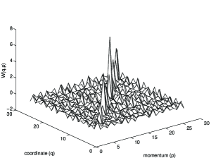
Figure 1: Localized pattern-like (waveleton) Wigner function.

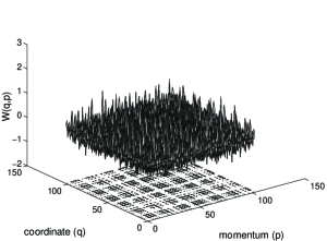
Figure 2: Entangled-like Wigner function.

Our (nonlinear) eigenmodes are more realistic for the modelling of nonlinear classical/quantum dynamical process than the corresponding linear gaussian-like coherent states. Here we mention only the best convergence properties of the expansions based on wavelet packets, which realize the minimal Shannon entropy property and the exponential control of convergence of expansions like (20) based on the norm (12). Figures 1, 2 present the solutions, constructed from the first 6 eigenmodes (6 levels in formula (20)), and demonstrate the stable localized pattern formation (waveleton) and complex entangled-like behaviour. Fig. 1 corresponds to (possible) result of superselection (einselection) [1] after decoherence process started from entangled pattern demonstrated on Fig. 2. It should be noted that we can control the type of behaviour on the level of the reduced algebraical variational system [2].

References

- [1] D. Sternheimer, arXiv: math. QA/9809056; W. P. Schleich, Quantum Optics in Phase Space, Wiley, 2000; S. de Groot, L Suttorp, Foundations of Electrodynamics, North-Holland, 1972
- [2] A.N. Fedorova and M.G. Zeitlin, Quantum Aspects of Beam Physics, Ed. P. Chen, 527, 539, World Scientific, Singapore, 2002; arXiv: physics/0101006, 0101007; quant-ph/0306197
- [3] Y. Meyer, Wavelets and Operators, Cambridge Univ. Press, 1990.