VIA MULTIRESOLUTION.

I. BBGKY HIERARCHY

Antonina N. Fedorova, Michael G. Zeitlin

IPME RAS, St. Petersburg, V.O. Bolshoj pr., 61, 199178, Russia

e-mail: zeitlin@math.ipme.ru

e-mail: anton@math.ipme.ru

http://www.ipme.ru/zeitlin.html

http://www.ipme.nw.ru/zeitlin.html A fast and efficient numerical-analytical approach is proposed for modeling complex behaviour in the BBGKY hierarchy of kinetic equations. We construct the multiscale representation for hierarchy of reduced distribution functions in the variational approach and multiresolution decomposition in polynomial tensor algebras of high-localized states. Numerical modeling shows the creation of various internal structures from localized modes, which are related to localized or chaotic type of behaviour and the corresponding patterns (waveletons) formation. The localized pattern is a model for energy confinement state (fusion) in plasma. Presented at IX International Workshop on Advanced

Computing and Analysis Techniques in Physics Research

ACAT03, December, 2003, KEK, Tsukuba, Japan Nuclear Instruments and Methods in Physics Research A, in press

Classical and Quantum Ensembles via Multiresolution.
I. BBGKY Hierarchy

Antonina N. Fedorova and Michael G. Zeitlin IPME RAS, St. Petersburg, V.O. Bolshoj pr., 61, 199178, Russia
E-mail: zeitlin@math.ipme.ru, anton@math.ipme.ru
http://www.ipme.ru/zeitlin.html, http://www.ipme.nw.ru/zeitlin.html

Abstract

A fast and efficient numerical-analytical approach is proposed for modeling complex behaviour in the BBGKY hierarchy of kinetic equations. We construct the multiscale representation for hierarchy of reduced distribution functions in the variational approach and multiresolution decomposition in polynomial tensor algebras of high-localized states. Numerical modeling shows the creation of various internal structures from localized modes, which are related to localized or chaotic type of behaviour and the corresponding patterns (waveletons) formation. The localized pattern is a model for energy confinement state (fusion) in plasma.

1 INTRODUCTION

Kinetic theory is an important part of general statistical physics related to phenomena which cannot be understood on the thermodynamic or fluid models level [1]. In these two papers we consider the applications of a new numerical/analytical technique based on wavelet analysis approach for calculations related to the description of complex (non-equilibrium) behaviour of the corresponding classical and quantum ensembles. The classical ensembles in this part are considered in the framework of the general BBGKY hierarchy and the quantum ones in part 2 in the Wigner-Weyl approach [1]. We restrict ourselves to the rational/polynomial type of nonlinearities (with respect to the set of all dynamical variables) that allows to use our results from [2], which are based on the so called multiresolution framework [3] and the variational formulation of initial nonlinear (pseudodifferential) problems. Wavelet analysis is a set of mathematical methods which give a possibility to work with well-localized bases in functional spaces and provide the maximum sparse forms for the general type of operators (differential, integral, pseudodifferential) in such bases. It provides the best possible rates of convergence and minimal complexity of algorithms inside and, as a result, saves CPU time and HDD space [3]. Our main goals are an attempt of classification and construction of a possible zoo of nontrivial (meta) stable states: (a) high-localized (nonlinear) eigenmodes, (b) complex (chaotic-like or entangled) patterns, (c) localized (stable) patterns (waveletons). In case (c) an energy is distributed during some time (sufficiently large) between only a few localized modes (from point (a)). We believe, it is a good image for plasma in a fusion state (energy confinement). Our construction of cut-off of the infinite system of equations is based on some criterion of convergence of the full solution. This criterion is based on a natural norm in the proper functional space, which takes into account (non-perturbatively) the underlying multiscale structure of complex statistical dynamics. In Sec. 2 the kinetic BBGKY hierarchy is formulated. In Sec. 3 we present the explicit analytical construction of solutions of the hierarchy, which is based on tensor algebra extensions of bases generated by the hidden multiresolution structure and proper variational formulation leading to an algebraic parametrization of the solutions. So, our approach resembles Bogolyubov’s and related approaches but we don’t use any perturbation technique (like virial expansion) or linearization procedures. Numerical modeling as in general case as in particular cases of the Vlasov-like equations shows the creation of various internal structures from localized bases modes, which demonstrate the possiblity of existence of (metastable) pattern formation.

2 BBGKY HIERARCHY

Let $M$ be the phase space of an ensemble of $N$ particles (${\rm dim}M=6N$) with coordinates $x_{i}=(q_{i},p_{i}),\quad i=1,...,N,\quad q_{i}=(q^{1}_{i},q^{2}_{i},q^{3}_{i})\in R^{3},\quad p_{i}=(p^{1}_{i},p^{2}_{i},p^{3}_{i})\in R^{3},\quad q=(q_{1},\dots,q_{N})\in R^{3N}$. Individual and collective measures are: $\mu_{i}=\mathrm{d}x_{i}=\mathrm{d}q_{i}\mathrm{d}p_{i},\quad\mu=\prod^{N}_{i=1}\mu_{i}$. Our constructions can be applied to the following general Hamiltonians: H_N= ∑^N_i=1(p2i2m+U_i(q))+ ∑_1≤i≤j≤NU_ij(q_i,q_j) where the potentials $U_{i}(q)=U_{i}(q_{1},\dots,q_{N})$ and $U_{ij}(q_{i},q_{j})$ are restricted to rational functions of the coordinates. Let $L_{s}$ and $L_{ij}$ be the Liouvillean operators (vector fields)

$$L_{s}=\sum^{s}_{j=1}\Big{(}\frac{p_{j}}{m}\frac{\partial}{\partial q_{j}}-\frac{\partial U_{j}}{\partial q}\frac{\partial}{\partial p_{j}}\Big{)}-\sum_{1\leq i\leq j\leq s}L_{ij}$$ (1)

$$L_{ij}=\frac{\partial U_{ij}}{\partial q_{i}}\frac{\partial}{\partial p_{i}}+\frac{\partial U_{ij}}{\partial q_{j}}\frac{\partial}{\partial p_{j}}$$

and $F_{N}(x_{1},\dots,x_{N};t)$ be the hierarchy of $N$-particle distribution function. satisfying the standard BBGKY–hierarchy ($V$ is the volume) [1]:

$$\frac{\partial F_{s}}{\partial t}+L_{s}F_{s}=\frac{1}{V^{s}}\int\mathrm{d}\mu_{s+1}\sum^{s}_{i=1}L_{i,s+1}F_{s+1}$$ (2)

In most cases, one is interested in a representation of the form $F_{k}(x_{1},\dots,x_{k};t)=\prod^{k}_{i=1}F_{1}(x_{i};t)+G_{k}(x_{1},\dots,x_{k};t)$ where $G_{k}$ are correlators. Additional reductions often lead to simplifications, the simplest one, $G_{k}=0$, corresponding to the Vlasov approximation. Such physically motivated ansatzes for $F_{k}$ formally replace the linear (in $F_{k}$) and pseudodifferential (in general case) infinite system (2) by a finite-dimensional but nonlinear system with polynomial nonlinearities (more exactly, multilinearities [3]). Our key point in the following consideration is the proper nonperturbative generalization of the perturbative multiscale approach of Bogolyubov.

3 MULTISCALE ANALYSIS

The infinite hierarchy of distribution functions satisfying system (2) in the thermodynamical limit is:

$$F=\{F_{0},F_{1}(x_{1};t),\dots,F_{N}(x_{1},\dots,x_{N};t),\dots\}$$ (3)

where $F_{p}(x_{1},\dots,x_{p};t)\in H^{p}$, $H^{0}=R,\quad H^{p}=L^{2}(R^{6p})$ (or any different proper functional space), $F\in$ $H^{\infty}=H^{0}\oplus H^{1}\oplus\dots\oplus H^{p}\oplus\dots$ with the natural Fock space like norm (guaranteeing the positivity of the full measure):

$$(F,F)=F^{2}_{0}+\sum_{i}\int F^{2}_{i}(x_{1},\dots,x_{i};t)\prod^{i}_{\ell=1}\mu_{\ell}.$$ (4)

First of all we consider $F=F(t)$ as a function of time only, $F\in L^{2}(R)$, via multiresolution decomposition which naturally and efficiently introduces the infinite sequence of the underlying hidden scales [3]. Because the affine group of translations and dilations generates multiresolution approach, this method resembles the action of a microscope. We have the contribution to the final result from each scale of resolution from the whole infinite scale of spaces. We consider a multiresolution decomposition of $L^{2}(R)$ [3] (of course, we may consider any different and proper for some particular case functional space) which is a sequence of increasing closed subspaces $V_{j}\in L^{2}(R)$ (subspaces for modes with fixed dilation value):

$$...V_{-2}\subset V_{-1}\subset V_{0}\subset V_{1}\subset V_{2}\subset...$$ (5)

The closed subspace $V_{j}(j\in{\bf Z})$ corresponds to the level $j$ of resolution, or to the scale j and satisfies the following properties: let $W_{j}$ be the orthonormal complement of $V_{j}$ with respect to $V_{j+1}$: $V_{j+1}=V_{j}\bigoplus W_{j}.$ Then we have the following decomposition:

$$\{F(t)\}=\bigoplus_{-\infty<j<\infty}W_{j}=\overline{V_{c}\displaystyle\bigoplus^{\infty}_{j=0}W_{j}}$$ (6)

in case when $V_{c}$ is the coarsest scale of resolution. The subgroup of translations generates a basis for the fixed scale number: ${\rm span}_{k\in Z}\{2^{j/2}\Psi(2^{j}t-k)\}=W_{j}.$ The whole basis is generated by action of the full affine group:

$${\rm span}_{k\in Z,j\in Z}\{2^{j/2}\Psi(2^{j}t-k)\}=$$ (7)

$${\rm span}_{k,j\in Z}\{\Psi_{j,k}\}=\{F(t)\}$$

Let the sequence $\{V_{j}^{t}\},V_{j}^{t}\subset L^{2}(R)$ correspond to multiresolution analysis on the time axis, $\{V_{j}^{x_{i}}\}$ correspond to multiresolution analysis for coordinate $x_{i}$, then $V_{j}^{n+1}=V^{x_{1}}_{j}\otimes\dots\otimes V^{x_{n}}_{j}\otimes V^{t}_{j}$ corresponds to the multiresolution analysis for the $n$-particle distribution function $F_{n}(x_{1},\dots,x_{n};t)$. E.g., for $n=2$: $V^{2}_{0}=\{f:f(x_{1},x_{2})=$ $\sum_{k_{1},k_{2}}a_{k_{1},k_{2}}\phi^{2}(x_{1}-k_{1},x_{2}-k_{2}),\ a_{k_{1},k_{2}}\in\ell^{2}(Z^{2})\},$ where $\phi^{2}(x_{1},x_{2})=\phi^{1}(x_{1})\phi^{2}(x_{2})=\phi^{1}\otimes\phi^{2}(x_{1},x_{2}),$ and $\phi^{i}(x_{i})\equiv\phi(x_{i})$ form a multiresolution basis corresponding to $\{V_{j}^{x_{i}}\}$. If $\{\phi^{1}(x_{1}-\ell)\},\ \ell\in Z$ form an orthonormal set, then $\phi^{2}(x_{1}-k_{1},x_{2}-k_{2})$ form an orthonormal basis for $V^{2}_{0}$. So, the action of the affine group generates multiresolution representation of $L^{2}(R^{2})$. After introducing the detail spaces $W^{2}_{j}$, we have, e.g. $V^{2}_{1}=V^{2}_{0}\oplus W^{2}_{0}.$ Then the 3-component basis for $W^{2}_{0}$ is generated by the translations of three functions: $\Psi^{2}_{1}=\phi^{1}(x_{1})\otimes\Psi^{2}(x_{2}),\Psi^{2}_{2}=\Psi^{1}(x_{1})\otimes\phi^{2}(x_{2}),\Psi^{2}_{3}=\Psi^{1}(x_{1})\otimes\Psi^{2}(x_{2}).$ Also, we may use the rectangle lattice of scales and one-dimensional wavelet decomposition: f(x_1,x_2)=∑_i,ℓ;j,k⟨f,Ψ_i,ℓ⊗Ψ_j,k⟩Ψ_j,ℓ⊗Ψ_j,k(x_1,x_2) where the basis functions $\Psi_{i,\ell}\otimes\Psi_{j,k}$ depend on two scales $2^{-i}$ and $2^{-j}$. We obtain our multiscale/multiresolution representations (formulae (11) below) via the variational wavelet approach for the following formal representation of the BBGKY system (9) (or its finite-dimensional nonlinear approximation for the $n$-particle distribution functions) with the corresponding obvious constraints on the distribution functions. Let $L$ be an arbitrary (non)linear differential/integral operator with matrix dimension $d$ (finite or infinite), which acts on some set of functions from $L^{2}(\Omega^{\otimes^{n}})$: $\quad\Psi\equiv\Psi(t,x_{1},x_{2},\dots)=\Big{(}\Psi^{1}(t,x_{1},x_{2},\dots),\dots$, $\Psi^{d}(t,x_{1},x_{2},\dots)\Big{)}$, $\quad x_{i}\in\Omega\subset{\bf R}^{6}$, $n$ is the number of particles:

$$L\Psi\equiv L(Q,t,x_{i})\Psi(t,x_{i})=0,$$ (8)

$$Q\equiv Q_{d_{0},d_{1},d_{2},\dots}(t,x_{1},x_{2},\dots,$$

$$\partial/\partial t,\partial/\partial x_{1},\partial/\partial x_{2},\dots,\int\mu_{k})=$$

$$\sum_{i_{0},i_{1},i_{2},\dots=1}^{d_{0},d_{1},d_{2},\dots}q_{i_{0}i_{1}i_{2}\dots}(t,x_{1},x_{2},\dots)$$

$$\Big{(}\frac{\partial}{\partial t}\Big{)}^{i_{0}}\Big{(}\frac{\partial}{\partial x_{1}}\Big{)}^{i_{1}}\Big{(}\frac{\partial}{\partial x_{2}}\Big{)}^{i_{2}}\dots\int\mu_{k}$$

Let us consider now the $N$ mode approximation for the solution as the following ansatz:

$$\Psi^{N}(t,x_{1},x_{2},\dots)=\sum^{N}_{i_{0},i_{1},i_{2},\dots=1}a_{i_{0}i_{1}i_{2}\dots}$$ (9)

$$A_{i_{0}}\otimes B_{i_{1}}\otimes C_{i_{2}}\dots(t,x_{1},x_{2},\dots)$$

We shall determine the expansion coefficients from the following conditions (different related variational approaches are considered in [2]):

$$\ell^{N}_{k_{0},k_{1},k_{2},\dots}\equiv$$ (10)

∫(LΨ^N)A_k_0(t)B_k_1(x_1)C_k_2(x_2)dtdx_1dx_2…=0 Thus, we have exactly $dN^{n}$ algebraical equations for $dN^{n}$ unknowns $a_{i_{0},i_{1},\dots}$. So, the solution is parametrized by the solutions of two sets of reduced algebraical problems, one is linear or nonlinear (depending on the structure of the operator $L$) and the rest are linear problems related to the computation of the coefficients of the algebraic equations (10). which can be found by using the compactly supported wavelet basis functions for the expansions (9). As a result the solution of the equations (2) has the following multiscale decomposition via nonlinear high-localized eigenmodes F(t,x_1,x_2,…)= ∑_(i,j)∈Z^2a_ijU^i⊗V^j(t,x_1,…)

$$V^{j}(t)=V_{N}^{j,slow}(t)+\sum_{l\geq N}V^{j}_{l}(\omega_{l}t),\ \omega_{l}\sim 2^{l}$$ (11)

U^i(x_s)= U_M^i,slow(x_s)+∑_m≥MU^i_m(k^s_mx_s),  k^s_m∼2^m which corresponds to the full multiresolution expansion in all underlying time/space scales. The formulae (11) give the expansion into a slow and fast oscillating parts. So, we may move from the coarse scales of resolution to the finest ones for obtaining more detailed information about the dynamical process. In this way one obtains contributions to the full solution from each scale of resolution or each time/space scale or from each nonlinear eigenmode. It should be noted that such representations give the best possible localization properties in the corresponding (phase)space/time coordinates. Formulae (11) do not use perturbation techniques or linearization procedures.

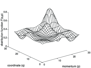
Figure 1: Localized mode contribution to distribution function.

Figure 2: Chaotic-like pattern.

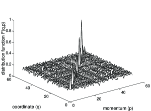
Figure 3: Localized waveleton pattern.

Numerical calculations are based on compactly supported wavelets and related wavelet families [3] and on evaluation of the accuracy on the level $N$ of the corresponding cut-off of the full system (2) regarding norm (4): $\|F^{N+1}-F^{N}\|\leq\varepsilon.$ We believe that the appearance of nontrivial localized patterns (a)-(c) demonstrated on Fig.1–Fig.3 constructed by these methods is a general effect which is also present in the full BBGKY hierarchy, due to its complicated intrinsic multiscale dynamics and it depends on neither the cut-off level nor the phenomenological-like hypothesis on correlators. So, representations like (11) and the prediction of the existence of the (asymptotically) stable localized patterns/states (energy confinement states) in BBGKY-like systems are the main results of this paper.

We are very grateful to Prof. Kaneko (KEK) and Prof. Perret-Gallix (CNRS) for kind help and attention during ACAT03 Workshop at KEK.

References

- [1] R. Balescu, Equilibrium and Nonequilibrium Statistical Mechanics, Wiley, New York, 1975.
- [2] A.N. Fedorova and M.G. Zeitlin, Progress in Nonequilibrium Green’s Functions II, Ed. M. Bonitz, 481, World Scientific, Singapore, 2003; arXiv: physics/0212066; quant-ph/0306197
- [3] Y. Meyer, Wavelets and Operators, Cambridge Univ. Press, 1990.