Characteristics of the Limit Cycle of a Reciprocating Quantum Heat Engine.

Abstract

When a reciprocating heat engine is started it eventually settles to a stable mode of operation. The approach of a first principle quantum heat engine toward this stable limit cycle is studied. The engine is based on a working medium consisting of an ensemble of quantum systems composed of two coupled spins. A four stroke cycle of operation is studied, with two isochore branches where heat is transferred from the hot/cold baths and two adiabats where work is exchanged. The dynamics is generated by a completely positive map. It has been shown that the performance of this model resembles an engine with intrinsic friction. The quantum conditional entropy is employed to prove the monotonic approach to a limit cycle. Other convex measures, such as the quantum distance display the same monotonic approach. The equations of motion of the engine are solved for the different branches and are combined to a global propagator that relates the state of the engine in the beginning of the cycle to the state after one period of operation of the cycle. The eigenvalues of the propagator define the rate of relaxation toward the limit cycle. A longitudinal and transverse mode of approach to the limit cycle is identified. The entropy balance is used to explore the necessary conditions which lead to a stable limit cycle. The phenomena of friction can be identified with a zero change in the von Neumann entropy of the working medium.

I Introduction

On starting up a reciprocating four stroke engine, after a few cycles, the engine settles to a limiting smooth cycle of operation. The present theoretical analysis is devoted to the characterization of the transition period from the state when the engine is started up to the sequence of states characterizing the periodic steady state termed the limit cycle. The process has similarities to the approach to thermodynamical equilibrium of an initially displaced state. This relaxation to equilibrium is accompanied by entropy production signifying the irreversible character of the process. Entropy is produced in the approach to the limit cycle but unlike an equilibrium state entropy continues to be produced also when the limit cycle is reached.

The approach to a limit cycle is based on the concept of a basin of attraction where the limit cycle is located at its minimum. The basin of attraction is set by external and internal constraints. Dissipative forces cause the system to settle down to the minimum of such a basin. A first principle study requires to determine the equations of motion governing the dynamics of the engine. For this task in the study, the framework of open quantum systems is employed Alicki and Lendi (1987); Lindblad (1976). The key point is that the dynamics of the engine is governed by a completely positive map Kraus (1971). Then the limit cycle becomes a fixed point of this map. In order to determine if the approach to the limit cycle is monotonic, a measure of distance between the actual state of the engine and the final limiting cycle has to be defined. Such a measure of distance between two quantum states is not obvious due to the possibility that the two states do not commute. In analogy to linear response theory it is expected that close enough to the limit cycle all distance measures should show the same relaxation rate toward the target limit cycle. This prediction is consistent with the results of the present study. Nevertheless at large distance from the limit cycle only the quantum measures show a monotonic approach to it.

The present paper is a continuation of a series of studies on a four stroke quantum engine Geva and Kosloff (1992); T. Feldmann and Salamon (1996); Feldmann and Kosloff (2000); Kosloff and Feldmann (2002); Feldmann and Kosloff (2003). The models studied were based on a first principle quantum description of the dynamics. The previous studies showed that the model engine displays the irreversible characteristics of common real heat engines operating in finite time. The performance of the quantum engine was found to be limited by finite heat transfer. In addition quantum performance limitations on the adiabatic branches mimicked very closely macroscopic friction phenomena Kosloff and Feldmann (2002).

The quantum discrete heat engine is composed of a quantum working fluid, a hot and a cold bath and an external field which can alter the energy levels of the working medium. The control parameters are the time allocations on the different branches, the total cycle time and the extreme values of the external field. All four branches are described by quantum equations of motion. The thermodynamical consequences can therefore be derived from first principles. A minimum set of three thermodynamical observables was found which were sufficient to characterize the performance of the engine. With two additional variables, the state of the working fluid could also be characterized Feldmann and Kosloff (2003). Knowledge of the state is necessary in order to evaluate the entropy and the internal temperature, variables which are necessary to establish a thermodynamic perspective.

The intuitive notion is that the limit cycle is characterized by the external constraints and internal properties of the engine. The following questions arise naturally:

• How do the control parameters characterize the approach to the limit cycle?

• Can conditions be found for the non-existence of a limit cycle?

• What are the irreversible properties of the limit cycle?

The present paper is devoted to the study of these issues in the context of quantum thermodynamics.

II Quantum Thermodynamical Observables and their Dynamics

In the field of quantum thermodynamics, thermodynamical variables are associated with quantum mechanical observables. An observable $\langle{\bf\hat{A}}\rangle$, is defined as the following scalar product between the operator ${\bf\hat{A}}$ and the density operator ${{\boldsymbol{\mathrm{\hat{\rho}}}}}$:

$$\langle{\bf\hat{A}}\rangle~{}=~{}\left({\bf\hat{A}}\cdot{{\boldsymbol{\mathrm{\hat{\rho}}}}}\right)~{}=~{}tr\{{\bf\hat{A}}^{{\dagger}}~{}{{\boldsymbol{\mathrm{\hat{\rho}}}}}\}~{}~{}~{}.$$ (1)

The dynamics of the quantum thermodynamical observables are described by completely positive maps within the formulation of quantum open systems Lindblad (1976); Alicki and Lendi (1987). The dynamics is generated by the Liouville super operator, which in the Heisenberg picture becomes:

$$\dot{\bf\hat{A}}~{}~{}=~{}~{}{\cal L}^{*}({\bf\hat{A}})~{}+~{}\frac{\partial{\bf\hat{A}}}{\partial t}~{}~{}~{}.$$ (2)

where ${\cal L}$ is a generator of a completely positive map: ${\cal T}(t)=e^{{\cal L}t}$. The generator ${\cal L}$ can be decomposed to the unitary and dissipative contributions ${\cal L}^{*}={\cal L}_{H}^{*}+{\cal L}_{D}^{*}$. The second term in Eq. (2) $\frac{\partial{\bf\hat{A}}}{\partial t}$, addresses a possible explicit time dependence of the operator.

The thermodynamical construction follows Gibbs by seeking a minimum set of variables associated with the quantum orthogonal observables $\{{\boldsymbol{\mathrm{\hat{B}}}}_{k}\}$. This set should be sufficient to completely determine the state of the system ${\boldsymbol{\mathrm{\hat{\rho}}}}$. In addition the set should be closed for the dynamics i.e for the operation of ${\cal L}^{*}$. Any cycle of a heat engine can be decomposed into a sequence of four completely positive maps defining the different branches. Eventually this sequence closes upon itself. A thermodynamical description therefore means that the set of variables should be closed for the dynamics during all branches of the operation. In equilibrium statistical mechanics the energy of a subsystem is sufficient to determine its state. In the present non-equilibrium example, additional variables $\langle{{\boldsymbol{\mathrm{\hat{B}}}}}_{k}\rangle$ are required to define the state of the working fluid. The set of time dependent expectation values $\vec{\bf b}(t)$ are used to reconstruct the density operator:

$${{\boldsymbol{\mathrm{\hat{\rho}}}}}~{}~{}=~{}~{}\frac{1}{N}{{\boldsymbol{\mathrm{\hat{I}}}}}+\sum_{\bf k}b_{\bf k}{{\boldsymbol{\mathrm{\hat{B}}}}_{k}}~{}~{}~{},$$ (3)

where the expansion coefficients become $b_{\bf k}=\langle{{\boldsymbol{\mathrm{\hat{B}}}}}_{k}\rangle$, $\left({{\boldsymbol{\mathrm{\hat{B}}}}}_{k}\cdot{{\boldsymbol{\mathrm{\hat{B}}}}}_{j}\right)=tr\{{\boldsymbol{\mathrm{\hat{B}}}}_{k}^{\dagger}{\boldsymbol{\mathrm{\hat{B}}}}_{j}\}=\delta_{kj}$, $tr\{{\boldsymbol{\mathrm{\hat{B}}}}_{k}\}=0$, and N is the size of the Hilbert space.

II.1 Quantum entropy

Thermodynamic measures require the knowledge of the state of the system ${\boldsymbol{\mathrm{\hat{\rho}}}}$. Entropy, the most common measure, is associated with the lack of knowledge or dispersion of the system Ruskai (2002); Vedral (2002). The entropy associated with a measurement of an observable $\langle{\bf\hat{A}}\rangle$ with $N$ possible outcomes becomes:

$$S_{{\boldsymbol{\mathrm{\hat{A}}}}}~{}~{}=~{}~{}-\sum_{j}^{N}p_{j}\log p_{j}~{}~{},$$ (4)

where $p_{j}=tr\{{\boldsymbol{\mathrm{\hat{P}}}}_{j}{\boldsymbol{\mathrm{\hat{\rho}}}}\}$ and ${\boldsymbol{\mathrm{\hat{P}}}}_{j}$ is the $j$ projection operator of the operator ${\boldsymbol{\mathrm{\hat{A}}}}=\sum_{j}^{N}\alpha_{j}{\boldsymbol{\mathrm{\hat{P}}}}_{j}$, and where the spectral decomposition (${\boldsymbol{\mathrm{\hat{A}}}}|\phi_{j}\rangle=\alpha_{j}|\phi_{j}\rangle$, ${\boldsymbol{\mathrm{\hat{P}}}}_{j}=|\phi_{j}\rangle\langle\phi_{j}|$) was utilized. Looking for the observable which complete measurement maximizes the information on the state, is equivalent to minimizing the entropy with respect to all possible observables. This process leads to the von Neumann entropy

$${\cal S}~{}~{}=~{}~{}-tr\{{\boldsymbol{\mathrm{\hat{\rho}}}}\log{\boldsymbol{\mathrm{\hat{\rho}}}}\}~{}~{},$$ (5)

and the optimum operator that minimizes dispersion commutes with the state ${\boldsymbol{\mathrm{\hat{\rho}}}}$.

The distance from a reference state ${\boldsymbol{\mathrm{\hat{\rho}}}}_{ref}$ is a key component in the study of the approach to the equilibrium or to the steady state. The conditional entropy is associated with the lack of information on the state ${\boldsymbol{\mathrm{\hat{\rho}}}}$ subject to the knowledge of a reference state ${\boldsymbol{\mathrm{\hat{\rho}}}}_{ref}$. The conditional entropy associated with a measurement of a particular observable becomes:

$${\cal S}_{{\boldsymbol{\mathrm{\hat{A}}}}}({\boldsymbol{\mathrm{\hat{\rho}}}}|{\boldsymbol{\mathrm{\hat{\rho}}}}_{ref})~{}~{}=~{}~{}-\sum_{j}p_{j}\log\frac{p_{j}}{q_{j}}~{}~{},$$ (6)

where $q_{j}=tr\{{\boldsymbol{\mathrm{\hat{P}}}}_{j}{\boldsymbol{\mathrm{\hat{\rho}}}}_{ref}\}$. The conditional entropy is bound from above and positive:

$${\cal S}_{{\boldsymbol{\mathrm{\hat{A}}}}}({\boldsymbol{\mathrm{\hat{\rho}}}})\geq S_{{\boldsymbol{\mathrm{\hat{A}}}}}({\boldsymbol{\mathrm{\hat{\rho}}}}|{\boldsymbol{\mathrm{\hat{\rho}}}}_{ref})~{}~{}.\geq 0$$ (7)

The value zero is reached only when ${\boldsymbol{\mathrm{\hat{\rho}}}}={\boldsymbol{\mathrm{\hat{\rho}}}}_{ref}$.

Maximizing Eq. (6) with respect to the operator ${\boldsymbol{\mathrm{\hat{A}}}}$, leads to an entropy measure which depends only on the two states:

$${\cal S}({\boldsymbol{\mathrm{\hat{\rho}}}}|{\boldsymbol{\mathrm{\hat{\rho}}}}_{ref})~{}~{}=~{}~{}-tr\{{\boldsymbol{\mathrm{\hat{\rho}}}}(\log{\boldsymbol{\mathrm{\hat{\rho}}}}-\log{\boldsymbol{\mathrm{\hat{\rho}}}}_{ref})\}~{}~{},$$ (8)

$S({\boldsymbol{\mathrm{\hat{\rho}}}}|{\boldsymbol{\mathrm{\hat{\rho}}}}_{ref})=0$ when the two states become indistinguishable.

II.2 Conditions for the monotonic approach to the limit cycle

Lindblad Lindblad (1975) has proven that the conditional entropy decreases if a completely positive map is applied to both the state ${\boldsymbol{\mathrm{\hat{\rho}}}}$ and the reference state ${\boldsymbol{\mathrm{\hat{\rho}}}}_{ref}$:

$${\cal S}({\boldsymbol{\mathrm{\hat{\rho}}}}|{\boldsymbol{\mathrm{\hat{\rho}}}}_{ref})~{}~{}\geq~{}~{}{\cal S}({\cal T}{\boldsymbol{\mathrm{\hat{\rho}}}}|{\cal T}{\boldsymbol{\mathrm{\hat{\rho}}}}_{ref})~{}~{},$$ (9)

where ${\cal T}$ is a completely positive map. An interpretation of Eq. (9) is that a completely positive map reduces the distinguishability between two states. This observation has been employed to prove the monotonic approach to equilibrium, provided that the reference state ${\boldsymbol{\mathrm{\hat{\rho}}}}_{ref}$ is the only invariant of the mapping $\cal T$ i.e. ${\cal T}{\boldsymbol{\mathrm{\hat{\rho}}}}_{ref}={\boldsymbol{\mathrm{\hat{\rho}}}}_{ref}$ Frigerio (1977, 1978).

The same reasoning can prove the monotonic approach to the limit cycle. The mapping imposed by the cycle of operation of a heat engine is a product of the individual evolution steps along the branches composing the cycle of operation (Cf. IV.3 ). Each one of these evolution steps is a completely positive map, so that the total evolution ${\cal U}_{cyc}$ that represents one cycle of operation, is also a completely positive map. If then a state ${{\boldsymbol{\mathrm{\hat{\rho}}}}}_{lc}$ is found that is a single invariant of ${\cal U}_{cyc}$ i.e. ${\cal U}_{cyc}{\boldsymbol{\mathrm{\hat{\rho}}}}_{lc}={\boldsymbol{\mathrm{\hat{\rho}}}}_{lc}$ then any initial state ${{\boldsymbol{\mathrm{\hat{\rho}}}}}_{init}$ will monotonically approach to the limit cycle. Based on Eq. (9) a monotonic decreasing series bound from below converges to a limit.

$$S({\boldsymbol{\mathrm{\hat{\rho}}}}_{init}|{\boldsymbol{\mathrm{\hat{\rho}}}}_{lc})\geq S({\cal U}_{cyc}{\boldsymbol{\mathrm{\hat{\rho}}}}_{init}|{\boldsymbol{\mathrm{\hat{\rho}}}}_{lc})\geq S({\cal U}_{cyc}^{n}{\boldsymbol{\mathrm{\hat{\rho}}}}_{init}|{\boldsymbol{\mathrm{\hat{\rho}}}}_{lc})~{}~{}\geq~{}~{}0~{}~{},$$ (10)

where ${\cal U}_{cyc}^{n}$ represents a sequential mapping of the cycle $n$ times.

The largest eigenvalue of ${\cal U}_{cyc}$ with a value of one is associated with the invariant limit cycle state ${\cal U}_{cyc}{{\boldsymbol{\mathrm{\hat{\rho}}}}}_{lc}={\bf 1}{\boldsymbol{\mathrm{\hat{\rho}}}}_{lc}$, the fixed point of ${\cal U}_{cyc}$. The other eigenvalues determine the rate of approach to the limit cycle (Cf. Sec. V.1)

The conditional entropy has been criticized as a measure of distance since it is not symmetric in ${\boldsymbol{\mathrm{\hat{\rho}}}}$ and ${\boldsymbol{\mathrm{\hat{\rho}}}}_{ref}$ and therefore does not form a metric. For this reason other measures have been defined.

II.3 Thermodynamic Quantum Distance

The concept of statistical distance between different pure quantum systems was introduced by W. K. Wootters Wootters (1981), who followed R. A. Fisher’s Fischer (1922) idea to measure distance in probability space. In Braunstein and Caves (1994) the concept of distinguishability for neighboring mixed quantum states is described. H$\ddot{u}$bner Hübner (1992) computed explicitly the distance between two-dimensional density operators, and gave a general formula for the N dimensional distance. A detailed and clear review on the subject has been presented by Diósi and Salamon Diósi and Salamon (1999).

II.3.1 Wootters Distance

Statistical distance is associated with the size of the statistical fluctuations occurring in a measurements that distinguishes one state from another. Two outcomes are distinguishable in a given number of trials, provided that the difference in actual probabilities is larger than the size of typical fluctuation. The maximal number of distinguishable states that can be found between two probability distributions has been suggested by Wootters Wootters (1981) to define the distance between these two states.

Consider two probability distributions $\bf p$ and $\bf q$ obtained from the same complete measurement of two quantum states ${\boldsymbol{\mathrm{\hat{\rho}}}}$ and ${\boldsymbol{\mathrm{\hat{\rho}}}}_{ref}$ (Cf. Eq. (6)). In order to define a distance between between $\bf p$ and $\bf q$ a continuous curve is sought connecting the two distributions. Taking advantage of normalization and that probabilities are positive, a change of variable is used: $x_{j}=\sqrt{p}_{j}$ and $y_{j}=\sqrt{q}_{j}$. The new variables allow a geometric interpretation, they define points on an $N$ dimensional unit sphere, since $\sum_{j}^{N}x_{j}^{2}=\sum_{j}^{N}y_{j}^{2}=1$. The statistical distance between $\bf p$ and $\bf q$ then becomes the shortest distance on the surface of this unit sphere between the points defined by the vectors $\bf x$ and $\bf y$. This shortest distance is equal to the angle between the unit vectors $\bf x$ and $\bf y$, given by:

$${\cal D}_{{\boldsymbol{\mathrm{\hat{A}}}}}({\bf p},{\bf q})~{}=~{}\arccos\left(\sum_{j=1}^{N}x_{j}y_{j}\right)~{}=~{}~{}~{}\arccos\left(\sum_{j=1}^{N}\sqrt{p_{j}}\sqrt{q_{j}}\right)~{}~{}~{}.$$ (11)

For quantum systems Eq. (11) corresponds to the statistical distance associated with a measurement of an operator ${\boldsymbol{\mathrm{\hat{A}}}}$. For two commuting states the statistical distance becomes the $\arccos$ of scalar product of the square roots of the density operators.

$${\cal D}({\boldsymbol{\mathrm{\hat{\rho}}}},{\boldsymbol{\mathrm{\hat{\rho}}}}_{ref})~{}=~{}~{}~{}\arccos\left(tr\left\{{\boldsymbol{\mathrm{\hat{\rho}}}}^{1/2}{\boldsymbol{\mathrm{\hat{\rho}}}}_{ref}^{1/2}\right\}\right)~{}~{}.$$ (12)

For two non-commuting states, the distance ${\cal D}({\boldsymbol{\mathrm{\hat{\rho}}}},{\boldsymbol{\mathrm{\hat{\rho}}}}_{ref})$ has to be redefined as Hübner (1992):

$${\cal D}({\boldsymbol{\mathrm{\hat{\rho}}}},{\boldsymbol{\mathrm{\hat{\rho}}}}_{ref})~{}=\sqrt{inf(tr\{({\boldsymbol{\mathrm{\hat{W}}}}_{1}-{\boldsymbol{\mathrm{\hat{W}}}}_{2})({\boldsymbol{\mathrm{\hat{W}}}}_{1}-{\boldsymbol{\mathrm{\hat{W}}}}_{2})^{*}\}}~{}~{},$$ (13)

where the infimum is taken over all Hilbert-Schmidt operators describing all the possible operators which fulfill

$${\boldsymbol{\mathrm{\hat{W}}}}_{1}{\boldsymbol{\mathrm{\hat{W}}}}_{1}^{*}={\boldsymbol{\mathrm{\hat{\rho}}}},~{}~{}{\boldsymbol{\mathrm{\hat{W}}}}_{2}{\boldsymbol{\mathrm{\hat{W}}}}_{2}^{*}={\boldsymbol{\mathrm{\hat{\rho}}}}_{ref}~{}~{},$$ (14)

and ${\boldsymbol{\mathrm{\hat{W}}}}_{1}^{*}{\boldsymbol{\mathrm{\hat{W}}}}_{2}>0$. This definition of distance is symmetric in ${\boldsymbol{\mathrm{\hat{\rho}}}}$, ${\boldsymbol{\mathrm{\hat{\rho}}}}_{ref}$ and therefore can form a metric Hübner (1992); Diósi and Salamon (1999):

$${\cal D}({\boldsymbol{\mathrm{\hat{\rho}}}},{\boldsymbol{\mathrm{\hat{\rho}}}}_{ref})~{}=~{}\sqrt{N\left(1~{}-~{}tr\sqrt{({\boldsymbol{\mathrm{\hat{\rho}}}})^{\frac{1}{2}}{\boldsymbol{\mathrm{\hat{\rho}}}}_{ref}({\boldsymbol{\mathrm{\hat{\rho}}}})^{\frac{1}{2}}}\right)}~{}~{},$$ (15)

where $N$ is the size of the Hilbert space.

II.4 Entropy production

Once the limit cycle is reached any observable is cyclic including the entropy. This is the result of the fact that the state of the system is completely determined by a finite number of expectation values which are cyclic. This means that entropy change in the complete cycle is zero or the total internal entropy production of the working medium is zero.

The external entropy production is positive for the limit cycle. It is a measure of the irreversible dissipation to the hot and cold baths:

$$\Delta{S}_{cyl}^{ext}~{}~{}=~{}~{}-\left(\frac{{\cal Q}_{h}}{T_{h}}+\frac{{\cal Q}_{c}}{T_{c}}\right)~{}~{},$$ (16)

where ${\cal Q}_{h/c}$ is the heat dissipated to the hot/cold bath and $T_{h/c}$ is the bath temperature.

III The quantum model

The present study is based on a four stroke quantum heat engine model corresponding to the Otto cycle. The cycle is composed of two isochores where the working medium is in contact with the hot/cold baths and the external field is constant and two adiabats where the external field is varying. The motion is generated by the Liouville operator $\cal L$ which can be decomposed to a Hamiltonian part and a dissipative part:

$${\cal L}^{*}~{}~{}=~{}{\cal L}_{H}^{*}+{\cal L}_{D}^{*}~{}~{},$$ (17)

where ${\cal L}_{H}^{*}{{\boldsymbol{\mathrm{\hat{A}}}}}=i[{{\boldsymbol{\mathrm{\hat{H}}}}},{{\boldsymbol{\mathrm{\hat{A}}}}}]$. The main feature of the Hamiltonian is that the external control part does not commute with the inertial internal part.

$${{\boldsymbol{\mathrm{\hat{H}}}}}~{}~{}=~{}~{}{{\boldsymbol{\mathrm{\hat{H}}}}}_{int}+{{\boldsymbol{\mathrm{\hat{H}}}}}_{ext}(t)~{}~{},$$ (18)

and $[{{\boldsymbol{\mathrm{\hat{H}}}}}_{int},{{\boldsymbol{\mathrm{\hat{H}}}}}_{ext}]~{}~{}\neq 0$.

The specific choice of working medium is composed of an ensemble of noninteracting coupled two-spin systems identical to the model studied in Ref. Feldmann and Kosloff (2003).

III.1 The Hamiltonian

The single particle Hamiltonian is chosen to be proportional to the polarization of a two-level-system (TLS): ${\boldsymbol{\mathrm{\hat{\sigma}}}}_{z}^{j}$. The operators ${\boldsymbol{\mathrm{\hat{\sigma}}}}_{z},{\boldsymbol{\mathrm{\hat{\sigma}}}}_{x},{\boldsymbol{\mathrm{\hat{\sigma}}}}_{y}$ are the Pauli matrices. For this system, the external Hamiltonian will be:

$${{\boldsymbol{\mathrm{\hat{H}}}}}_{ext}~{}~{}=~{}~{}2^{-3/2}\omega(t)\left({\boldsymbol{\mathrm{\hat{\sigma}}}}_{z}^{1}\otimes{\bf\hat{I}^{2}}+{\bf\hat{I}^{1}}\otimes{{{{\boldsymbol{\mathrm{\sigma}}}}}_{z}^{2}}\right)~{}\equiv~{}\omega(t){{\boldsymbol{\mathrm{\hat{B}}}}_{1}}~{}~{},$$ (19)

and the external control field $\omega(t)$ is chosen to be in the $z$ direction. The uncontrolled interaction Hamiltonian is chosen to be restricted to the coupling of pairs of spin atoms. Therefore the working fluid consists of noninteracting pairs of TLS’s. For simplicity, a single pair can be considered. The thermodynamics of $M$ pairs then follows by introducing a trivial scale factor. Accordingly let the uncontrolled part be:

$${{\boldsymbol{\mathrm{\hat{H}}}}}_{int}~{}~{}=~{}~{}2^{-3/2}J\left({{\boldsymbol{\mathrm{\hat{\sigma}}}}_{x}^{1}}\otimes{{\boldsymbol{\mathrm{\hat{\sigma}}}}_{x}^{2}}-{{\boldsymbol{\mathrm{\hat{\sigma}}}}_{y}^{1}}\otimes{\boldsymbol{\mathrm{\hat{\sigma}}}}_{y}^{2}~{}~{}~{}.\right)~{}\equiv~{}J{{\boldsymbol{\mathrm{\hat{B}}}}_{2}}~{}~{}.$$ (20)

$J$ scales the strength of the interaction. When $J\rightarrow 0$, the model represents a working medium with noninteracting atoms T. Feldmann and Salamon (1996).

The commutation relation: $[{{\boldsymbol{\mathrm{\hat{B}}}}}_{1},{{\boldsymbol{\mathrm{\hat{B}}}}}_{2}]=\sqrt{2}i{{\boldsymbol{\mathrm{\hat{B}}}}}_{3}$ leads to the definition of ${{\boldsymbol{\mathrm{\hat{B}}}}}_{3}$. The analysis shows Feldmann and Kosloff (2003), that the set of operators ${{\boldsymbol{\mathrm{\hat{B}}}}}_{1},{{\boldsymbol{\mathrm{\hat{B}}}}}_{2},{{\boldsymbol{\mathrm{\hat{B}}}}}_{3}$ and ${{\boldsymbol{\mathrm{\hat{I}}}}}$ forms a closed sub-algebra of the total Lie algebra of the combined system. The Hamiltonian expressed in terms of the operators ${{\boldsymbol{\mathrm{\hat{B}}}}_{1}},{{\boldsymbol{\mathrm{\hat{B}}}}_{2}},{{\boldsymbol{\mathrm{\hat{B}}}}_{3}}$ in the polarization representation becomes:

$$\begin{array}[]{c}{\bf\hat{H}}\end{array}~{}~{}=~{}~{}\begin{array}[]{c}\omega(t){\bf\hat{B}_{1}}+\rm J{\bf\hat{B}_{2}}~{}~{}.\end{array}$$ (23)

The eigenvalues of ${\boldsymbol{\mathrm{\hat{H}}}}$ are $0~{},~{}\pm\frac{\Omega}{\sqrt{2}}$ where $\Omega=\sqrt{\omega^{2}+J^{2}}$. The closed Lie algebra of the set $\{{\boldsymbol{\mathrm{\hat{B}}}}_{k}\}$ means that it is also closed for the propagation generated by the Hamiltonian (23).

IV The Cycle of Operation, the Quantum Otto cycle

The operation of the heat engine is determined by the properties of the working medium and the coupling to the hot and cold baths. The cycle of operation is defined by the external controls which include the variation in time of the field with the periodic property $\omega(t)=\omega(t+\tau)$ where $\tau$ is the total cycle time synchronized with the contact times on the different branches of the cycle. The cycle studied is composed of two branches where the working medium is in contact with the hot/cold baths and the field is constant, termed isochores. In addition, there are two branches where the field $\omega(t)$ varies and the working medium is disconnected from the baths termed adiabats. This cycle is a quantum analogue of the Otto cycle. The four strokes of the cycle with the corresponding parameters are (Cf. Fig. 1):

1. Isochore $A\rightarrow B$: the field is maintained constant $\omega=\omega_{b}$ while the working medium is in contact with the hot bath of temperature $T_{h}$ with heat conductance $\Gamma_{h}$, and dephasing parameter $\gamma_{h}$ for a period of $\tau_{h}$.

2. Adiabat $B\rightarrow C$: The field changes linearly from $\omega_{b}$ to $\omega_{a}$ in a time period of $\tau_{ba}$.

3. Isochore $C\rightarrow D$: the field is maintained constant $\omega=\omega_{a}$ the working medium is in contact with the cold bath of temperature $T_{c}$ with heat conductance $\Gamma_{c}$, and dephasing parameter $\gamma_{c}$ for a period of $\tau_{c}$.

4. Adiabat $D\rightarrow A$: The field changes linearly from $\omega_{a}$ to $\omega_{b}$ in a time period of $\tau_{ab}$.

Fig. 1 displays a typical trajectory of the cycle in the plane defined by the external field and the entropy ($\omega,{\cal S}_{E}$).

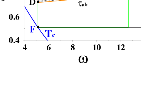
Figure 1: The cycle of the heat engine in the ($\omega,{\cal S}_{E}$) plane. The upper red line indicates the energy entropy of the working medium in equilibrium with the hot bath at temperature T_h for different values of the field. The blue line below indicates the energy entropy in equilibrium with the cold bath at temperature T_c. The cycle in green has an infinite time allocation on all branches. It reaches the equilibrium point with the hot bath (point E) and equilibrium point with the cold bath (point F). The inner cycle ABCD is a typical cycle with the time allocations: $\tau_{h}=2.5~{}\tau_{ba}=0.01,~{}\tau_{c}=3.~{}~{}\tau_{ab}=0.01$. The external parameters are: $\omega_{a}=5.08364,~{}\omega_{b}=12.6355,~{}J=2.,~{}T_{h}=7.5,~{}T_{c}=1.5,~{}\Gamma_{h}=~{}\Gamma_{c}=0.3423,~{}\gamma_{h}=\gamma_{c}=0$

The state ${\boldsymbol{\mathrm{\hat{\rho}}}}$ (Cf. Eq. (3)) of the working medium is completely reconstructed by the set $\{{{\boldsymbol{\mathrm{\hat{B}}}}_{k}}\}~{},k=1,5$ of five operators Feldmann and Kosloff (2003). The set of the three operators ${\bf\hat{B}_{1}},{\bf\hat{B}_{2}},{\bf\hat{B}_{3}}$ is sufficient to describe the energy changes during the cycle of operation. The map $\cal U$ relates the initial values of these operators to their final values for each of the engine branches. Implicitly this map is obtainable by solving a set of coupled inhomogeneous equations of motion for each branch Feldmann and Kosloff (2003). An explicit description of the map is obtained by adding the identity operator ${\boldsymbol{\mathrm{\hat{I}}}}$ which transforms the inhomogeneous equations to a closed set of linear coupled $4\times 4$ equations. The equation of motion of the two additional operators ${\bf\hat{B}_{4}}$ and ${\bf\hat{B}_{5}}$ form a linear first order inhomogeneous equation depending on the time dependence of the closed set ${\bf\hat{B}_{1}},{\bf\hat{B}_{2}},{\bf\hat{B}_{3}}$ and ${\bf\hat{I}}$. As a result they form an additional $2\times 2$ block in the map.

IV.1 Propagators on the isochores

The dynamical map ${\cal U}(\tau_{c/h})$ on the isochores is generated by both the Hamiltonian and the dissipative Lindblad generators representing the interaction with the bath. The $4\times 4$ block of the map is first solved for the set ${\bf\hat{B}_{1}},{\bf\hat{B}_{2}},{\bf\hat{B}_{3}}$ and ${\boldsymbol{\mathrm{\hat{I}}}}$. Since $\omega$ is constant on the isochores a closed form of the propagator ${\cal U}(\tau_{c/h})$ is obtained Feldmann and Kosloff (2003):

$$\begin{array}[]{c}{\cal U}(\tau_{c/h})=\end{array}\left(\begin{array}[]{cccc}K\frac{X\omega^{2}+c{J^{2}}}{{\Omega}^{2}}&K\frac{{\omega}J(X-c)}{{\Omega}^{2}}&K\frac{Js}{\Omega}&b_{1}^{eq}(1-e^{-\Gamma\tau_{c/h}})\\ K\frac{{\omega}J(X-c)}{{\Omega}^{2}}&K\frac{XJ^{2}+c{\omega}^{2}}{{\Omega}^{2}}&-K\frac{{\omega}s}{\Omega}&b_{2}^{eq}(1-e^{-\Gamma\tau_{c/h}})\\ -K\frac{Js}{\Omega}&K\frac{{\omega}s}{\Omega}&Kc&0\\ 0&0&0&1\\ \end{array}\right)~{}~{}~{},$$ (29)

where $K=\exp\{-(\Gamma+2\gamma\Omega^{2})\tau_{c/h}\}$, $X=\exp({2\gamma\Omega^{2}\tau_{c/h}})$, $c=\cos(\sqrt{2}\Omega\tau_{c/h})$ and $s=\sin(\sqrt{2}\Omega\tau_{c/h})$, $b_{1}^{eq}=-\frac{\omega}{\sqrt{2}\Omega\Gamma}(k\uparrow-k\downarrow)$, $b_{2}^{eq}=-\frac{J}{\sqrt{2}\Omega\Gamma}(k\uparrow-k\downarrow)$. Finally $\gamma$ is the dephasing constant, $\tau_{c/h}$ is the time spent on the cold/hot isochore , and $\Gamma=k\uparrow+k\downarrow$ is the heat-conductance to the bath. The corresponding bath temperature $T_{c/h}$, enters through the detailed balance relation: $\frac{k\uparrow}{k\downarrow}~{}~{}=~{}~{}e^{-\frac{\Omega}{T\sqrt{2}}}$. The block containing ${\boldsymbol{\mathrm{\hat{B}}}}_{4}$ and ${\boldsymbol{\mathrm{\hat{B}}}}_{5}$ can now be solved as a $2\times 2$ set of coupled inhomogeneous equation of motion Feldmann and Kosloff (2003).

IV.2 Propagators on the adiabats

The propagator on the adiabats is more involved. This is due to the explicit time dependence of the Hamiltonian. Using the Lie algebra of the set of $\{{\boldsymbol{\mathrm{\hat{B}}}}_{k}\}$ operators it is always possible Wei and Norman (1963) to describe the propagator as:

$${\boldsymbol{\mathrm{\hat{A}}}}(t)~{}~{}=~{}~{}{\boldsymbol{\mathrm{\hat{U}}}}{\boldsymbol{\mathrm{\hat{A}}}}{\boldsymbol{\mathrm{\hat{U}}}}^{\dagger}~{}~{},$$ (30)

where ${\boldsymbol{\mathrm{\hat{U}}}}=\exp(i\alpha_{1}(t){{\boldsymbol{\mathrm{\hat{B}}}}_{1}})\exp(i\alpha_{2}(t){{\boldsymbol{\mathrm{\hat{B}}}}_{2}})\exp(i\alpha_{3}(t){{\boldsymbol{\mathrm{\hat{B}}}}_{3}})$ and the coefficients $\alpha_{i}(t)$ include the effect of time ordering. The procedure is described in Appendix A. This approach leads to the explicit result for the propagator of the set ${\bf\hat{B}_{1}},{\bf\hat{B}_{2}},{\bf\hat{B}_{3}},{\bf\hat{I}}$:

$${\cal U}_{a}(t)~{}~{}=~{}~{}\left(\begin{array}[]{cccc}c_{2}c_{3}&-s_{3}c_{1}+c_{3}s_{2}s_{1}&c_{3}s_{2}c_{1}+s_{3}s_{1}&0\\ c_{2}s_{3}&c_{3}c_{1}+s_{3}s_{2}s_{1}&s_{3}s_{2}c_{1}-c_{3}s_{1}&0\\ -s_{2}&c_{2}s_{1}&c_{2}c_{1}&0\\ 0&0&0&1\\ \end{array}\right)~{}~{}~{},$$ (35)

where: $s_{1}=\sin(\alpha_{1}),~{}s_{2}=\sin(\alpha_{2}),~{}s_{3}=\sin(\alpha_{3})$,  $c_{1}=\cos(\alpha_{1}),~{}c_{2}=\cos(\alpha_{2}),~{}c_{3}=\cos(\alpha_{3})$. The coefficients $\alpha$ can be integrated either numerically Cf. Eq. (63) or closed form solutions are obtained for specific functional forms of $\omega(t)$ Feldmann and Kosloff (2003). The operators ${\boldsymbol{\mathrm{\hat{B}}}}_{4}$ and ${\boldsymbol{\mathrm{\hat{B}}}}_{5}$ commute with the Hamiltonian, and therefore are constant on the adiabats .

IV.3 The global propagator

The propagator of the cycle represents the completely positive map of the initial expectation values to the final ones after the operation of one cycle. The propagator is then constructed as a sequential product of the individual propagators on the different branches:

$${\cal U}_{cyc}={\cal U}_{ab}~{}{\cal U}_{isc}~{}{\cal U}_{ba}~{}{\cal U}_{ish}~{}~{}.$$ (36)

An analytic form has been obtained for the propagators on the isochores (Eq. (29)). For the adiabats the form of Eq. (35) has been used which is parametrically dependent on the $\alpha$ parameters.

Table I summarizes all the control parameters defining the cycle.

Table 1: Summary of notations

$T_{c}$	temperature of the cold bath.
$T_{h}$	temperature of the hot bath.
$\omega_{a}$	value of the external field at the cold isochore.
$\omega_{b}$	value of the external field at the hot isochore.
$J$	internal coupling constant.
$\Gamma_{c}$	heat transfer coupling constant to the cold bath.
$\Gamma_{h}$	heat transfer coupling constant to the cold bath.
$\gamma_{c}$	dephasing constant on the cold bath.
$\gamma_{c}$	dephasing constant on the hot bath.
$\tau_{c}$	time allocation on the cold isochore.
$\tau_{h}$	time allocation on the hot isochore.
$\tau_{ab}$	time allocation on the cold-to-hot adiabat.
$\tau_{ba}$	time allocation on the hot-to-cold adiabat.

The global map enable to solve for the operator expectation values from their initial values. These expectation values serve to reconstruct the density operator (Cf. Eq. (3) ) Feldmann and Kosloff (2003):

$$\begin{array}[]{c}{{\boldsymbol{\mathrm{\hat{\rho}}}}_{p}}\end{array}~{}~{}=~{}~{}~{}\left(\begin{array}[]{cccc}\frac{1}{4}+\frac{{b_{1}}}{\sqrt{2}}+\frac{b_{5}}{2}&0&0&\frac{{b_{2}}}{\sqrt{2}}-i\frac{{b_{3}}}{\sqrt{2}}\\ 0&\frac{1}{4}+\frac{b_{4}}{\sqrt{2}}-\frac{b_{5}}{2}&0&0\\ 0&0&\frac{1}{4}-\frac{b_{4}}{\sqrt{2}}-\frac{b_{5}}{2}&0\\ \frac{{b_{2}}}{\sqrt{2}}+i\frac{{b_{3}}}{\sqrt{2}}&0&0&\frac{1}{4}-\frac{b_{1}}{\sqrt{2}}+\frac{b_{5}}{2}\\ \end{array}\right)~{}~{}~{},$$ (42)

where the index $p$ stands for the direct product spin representation. Diagonalizing the density operator ${{\boldsymbol{\mathrm{\hat{\rho}}}}_{p}}$ Cf. Appendix B, leads to the eigenvalues of ${{\boldsymbol{\mathrm{\hat{\rho}}}}}$ which define the von Neumann probabilities:

$$\begin{array}[]{c}\lambda_{1}~{}=~{}\frac{1}{4}-\frac{D}{\sqrt{2}}+\frac{b_{5}}{2}\\ \lambda_{2}~{}=~{}\frac{1}{4}+\frac{b_{4}}{\sqrt{2}}-\frac{b_{5}}{2}\\ \lambda_{3}~{}=~{}\frac{1}{4}-\frac{b_{4}}{\sqrt{2}}-\frac{b_{5}}{2}\\ \lambda_{4}~{}=~{}\frac{1}{4}+\frac{D}{\sqrt{2}}+\frac{b_{5}}{2}\end{array}~{}~{},$$ (47)

where $D~{}=~{}\sqrt{b_{1}^{2}+b_{2}^{2}+b_{3}^{2}}$. Functionals of the density operator such as entropy are calculated by the spectral theorem Cf. appendix A.

V Limit Cycles

The heat engine’s limit cycle is completely determined by the external control parameters. This means that irrespective of the initial state of the working medium, after running the engine through many cycles of the control sequence, a limit cycle is approached. This can be observed in Fig. 2 which demonstrates that starting from two initial conditions, the engine settles to the same limit cycle which is the fixed point at the bottom of the basin of attraction.

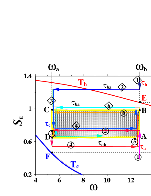
Figure 2: The limit cycle in the field entropy variables $(\omega,{\cal S}_{E})$. Two initial states represented by points are indicated by 1 with the field value of $\omega_{b}$. The sequence of branches starting from a cold initial temperature are shown with circles around the numbers. The working medium of the engine is put in contact with the hot bath for a time duration of $\tau_{h}$ and heats up. For time $\tau_{ba}$ the frequency changes from $\omega_{b}$ to $\omega_{a}$ (branch 2). Cooling due to contact with the cold bath is found on branch 3. For clarity the arrows do not reach the values of $\omega_{a}$ and $\omega_{b}$. The sequence of branches starting from a hot initial temperature are shown with diamonds around the numbers. The working medium of the engine is put in contact with the hot bath for a time duration of $\tau_{h}$ and cools down to branch 2. The contact with the cold branch further cools the engine (branch 3) After going through approximately 3 cycles of the engine, the two paths appear to converge to the same limit cycle, indicated by the ABCD rectangle.

V.1 Approach to the limit cycle

The timescale of the approach of the engine to the limit cycle is related to the number of accumulated cycles $n$, that are required for the variables of the engine to approach their asymptotic values. The different measures employed for this task are defined in Sec. II. The energy distance ${\cal D}_{E}({\boldsymbol{\mathrm{\hat{\rho}}}}_{n},{\boldsymbol{\mathrm{\hat{\rho}}}}_{lc})$ Eq. (11) and quantum distance ${\cal D}({\boldsymbol{\mathrm{\hat{\rho}}}}_{n},{\boldsymbol{\mathrm{\hat{\rho}}}}_{lc})$ were used as measures and are shown in Fig. 3. The reference state ${\boldsymbol{\mathrm{\hat{\rho}}}}_{lc}$ can be chosen on any point on the engine’s trajectory, on points A  B  C  D for example or between them. The same point on the trajectory is used to define the state in the n’th iteration ${\boldsymbol{\mathrm{\hat{\rho}}}}_{n}$. It was found that the distances are invariant to the choice of the chosen point on the cycle’s trajectory.

Explicitly the quantum distance , ${\cal D}({\boldsymbol{\mathrm{\hat{\rho}}}}_{n},{\boldsymbol{\mathrm{\hat{\rho}}}}_{lc})$, Eq. (15) for the current working medium becomes:

$${\cal D}({\boldsymbol{\mathrm{\hat{\rho}}}}_{n},{\boldsymbol{\mathrm{\hat{\rho}}}}_{lc})=\sqrt{2\left(1-(\sqrt{\zeta_{1}}+\sqrt{\lambda_{2}(n)\lambda_{3}(lc)}+\sqrt{\lambda_{3}(n)\lambda_{3}(lc)}+\sqrt{\zeta_{4}})\right)}~{}~{},$$ (48)

where the normalization is chosen to be $N=2$ and the eigenvalues $\lambda$ are the eigenvalues of the density operator defined in Eq. (47) and,

$$\zeta_{1,4}~{}=~{}Q\pm\sqrt{\left(\frac{YD_{n}}{\sqrt{2}}\right)^{2}+\left(\frac{x_{n}D_{lc}}{\sqrt{2}}\right)^{2}+2x_{n}qY}~{}~{},$$ (49)

where $2q$ is the scalar product between the $\{{\boldsymbol{\mathrm{\hat{B}}}}\}$ components:

$$2q=\left(\vec{b}_{n}\cdot\vec{b}_{lc}\right)=\sum_{j=1}^{3}b_{j}(n)b_{j}(lc)~{}~{},$$ (50)

and $x=\sqrt{\lambda_{1}\lambda_{4}}$, $2r=\frac{1}{2}+b_{5}$, $y=2(r-x)/D$, $Y=r_{lc}+qy_{n}$ and finally $Q$ is the generalized scalar product: $Q=r_{n}\cdot r_{lc}+q$, ($D$ is defined by following Eq. (47)). Additional computational details are given in Appendix B.2.

The distance to the limit cycle can also be associated with the conditional entropy:

$$\begin{array}[]{l}S({\boldsymbol{\mathrm{\hat{\rho}}}}_{n}|{\boldsymbol{\mathrm{\hat{\rho}}}}_{lc})={\cal S}({\boldsymbol{\mathrm{\hat{\rho}}}}_{n})-\\ \left(\{r_{n}-\frac{\sqrt{2}q}{D_{lc}}\}\log(\lambda_{1}({lc}))+\lambda_{2}(n)\log(\lambda_{2}({lc}))+\lambda_{3}(n)\log(\lambda_{3}(lc))+\{r_{n}+\frac{\sqrt{2}q}{D_{lc}}\}\log(\lambda_{1}(lc))\right)~{}~{},\end{array}$$

(53)

which becomes zero when ${\boldsymbol{\mathrm{\hat{\rho}}}}_{n}$ approaches the limit cycle.

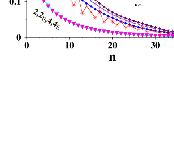
Figure 3: The distance ${\cal D}({\boldsymbol{\mathrm{\hat{\rho}}}}_{n},{\boldsymbol{\mathrm{\hat{\rho}}}}_{lc})$ and the energy distance ${\cal D}_{E}({\boldsymbol{\mathrm{\hat{\rho}}}}_{n},{\boldsymbol{\mathrm{\hat{\rho}}}}_{lc})$ from the limit cycle as a function of accumulated cycles $n$. Four example are shown numbered from 1 to 4. The corresponding inserts show the limit cycle in the energy entropy ${\cal S}_{E}$ and $\omega$ plane. The dashed lines indicated by $E$ correspond to the energy distance ${\cal D}_{E}({\boldsymbol{\mathrm{\hat{\rho}}}}_{n},{\boldsymbol{\mathrm{\hat{\rho}}}}_{lc})$. Cycles 1 and 3 are without dephasing. Cycle 2 and 4 include dephasing on the isochores with $\gamma_{h}=0.01$ and $\gamma_{c}=0.03$. All cycles spend the same time on the isochores ($\tau_{h}=\tau_{c}=0.6$). The time on the adiabats varies form very short, cycles 1 and 2, to very long, cycles 3 and 4.

In all cases studied the quantum distance ${\cal D}({\boldsymbol{\mathrm{\hat{\rho}}}}_{n},{\boldsymbol{\mathrm{\hat{\rho}}}}_{lc})$ monotonically approaches zero with the increase in the number $n$ of accumulated cycles,  Cf. Fig. 3. This was found also to be true for the conditional entropy as predicted by Eq. (10). The energy distance ${\cal D}_{E}({\boldsymbol{\mathrm{\hat{\rho}}}}_{n},{\boldsymbol{\mathrm{\hat{\rho}}}}_{lc})$ as in case $1_{E}$ in Fig. 3, shows a non-monotonic periodic oscillations in the approach to the limit cycle. With sufficient dephasing the density operator is almost diagonal in the energy representation therefore the two distances converge; ${\cal D}({\boldsymbol{\mathrm{\hat{\rho}}}}_{n},{\boldsymbol{\mathrm{\hat{\rho}}}}_{lc})={\cal D}_{E}({\boldsymbol{\mathrm{\hat{\rho}}}}_{n},{\boldsymbol{\mathrm{\hat{\rho}}}}_{lc})$ Cf. cases 2 and 4 in Fig. 3.

Examining the measures of approach to the limit cycle Eq. (48) and (53), it is found that they have similar functional dependence on the expectation values of the set of $\{{\boldsymbol{\mathrm{\hat{B}}}}\}$ operators. In particular the two functionals contain the scalar product $q$. This indicates that all quantum convex functionals of ${\boldsymbol{\mathrm{\hat{\rho}}}}$ will relax to the limit cycle in the same rate.

The dynamics of the set of operators $\{{\boldsymbol{\mathrm{\hat{B}}}}\}$ is determined by the eigenvalues of the Global Operator , ${\cal U}_{cyc}$, Eq. (36). The eigenvector with the eigenvalue of $\mu_{0}=1$ represents the expectation values of the limit cycle. The decay rate to the limit cycle depends on the eigenvalues which are smaller than one. The eigenvalue $\mu_{1}\leq 1$ was found to be real and as expected its eigenvector does not include a component of the identity operator. Fig. 4 shows the dependence of the eigenvalues $\mu$ of the Global Operator on the time spent on the isochores and the coupling constants. The relationship is well fitted by $\mu_{1}=e^{-(\Gamma_{h}\tau_{h}+\Gamma_{c}\tau_{c})}$. This means that a very weak dependence on the dephasing rate $\gamma_{h/c}$ was found. $\mu_{1}$ can then be interpreted as the relaxation rate per cycle in the direction defined by the limit cycle vector. The eigenvalues $\mu_{2/3}=|\mu_{2}|e^{\pm i\phi}$ are complex. Their amplitude can be fitted to $|\mu_{2/3}|=e^{-\left((\Gamma_{h}+\gamma_{h}\Omega_{h}^{2})\tau_{h}+(\Gamma_{c}+\gamma_{c}\Omega_{c}^{2})\tau_{c}\right)}$. This suggests that $\mu_{2/3}$ represents the rate of decay in a direction perpendicular to the direction of limit cycle vector. The phase $\phi$ of $\mu_{2/3}$ is an accumulated phase and was found to be linearly related to the time allocated on the adiabats. The last two eigenvalues associated with the block of ${\boldsymbol{\mathrm{\hat{B}}}}_{4}$ and ${\boldsymbol{\mathrm{\hat{B}}}}_{5}$ become $\mu_{4}=\mu_{1}$ and $\mu_{5}=(\mu_{1})^{2}$ ( Eq. (57) and (59) of Feldmann and Kosloff (2003) ).

The analysis reveals that the rate of approach to the limit cycle is determined by the accumulated dissipation on the the hot and cold isochores. The eigenvalue $\mu_{1}$ plays the role of the longitudinal relaxation analogue to $1/T_{1}$, while the eigenvalues $\mu_{2/3}$ play the role of the transverse relaxation or $1/T_{2}$.

Figure 4: Logarithms of the eigenvalues of the global propagator ${\cal U}_{cyc}$. Upper panel $\mu_{1}$ as a function of the accumulated relaxation $\Gamma_{h}\tau_{h}+\Gamma_{c}\tau_{c}$, the sum of the products of the coupling to the heat/cold baths, $\Gamma_{h/c}$, with the time allocation on the corresponding isochore, $\tau_{h/c}$. The eigenvalue is independent of the time allocation on the adiabats. Lower panel $\mu_{2/3}$ as a function of the accumulated dephasing $(\Gamma_{h}+2\gamma_{h}\Omega_{h}^{2})\tau_{h}+(\Gamma_{c}+2\gamma_{c}\Omega_{c}^{2})\tau_{c}$. The points on the graphs represent different choices of parameters and time allocation on the branches.

V.2 Properties of the limit cycle

The fact that the limit cycle is closed imposes a strict periodic constraint on all properties of the working medium. The periodicity of the energy entropy and the von Neumann entropy are a key to the understanding of the cycle performance.

V.2.1 Minimal cycle time

A limit cycle can only exist if the total internal entropy changes on the four branches sums up to zero. What combinations of control parameters such as the time allocations lead to a stable limit cycle? This question can be addressed by searching for the opposite conditions where a limit cycle cannot be closed. As was described in Sec. II.2 a limit cycle is obtained only when there is a single invariant of the propagator ${\cal U}_{cyl}$. An extreme case is when no time is allocated to the hot and cold isochores ($\tau_{c}=\tau_{h}=0$). By construction the map ${\cal U}_{cyl}$ is unitary and all eigenvalues are modulus 1. Thus any initial state will oscillate indefinitely without settling to a limit cycle. The next step in the investigation is to allocate some time to the cold isochore $\tau_{c}\neq 0$ adding a dissipative branch.

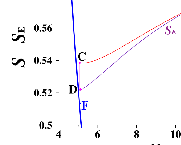
Figure 5: The energy entropy ${\cal S}_{E}$ and the von Neumann entropy ${\cal S}$ as a function of the field $\omega$ for a limit cycle with time allocations on the adiabats ($\tau_{ba}=\tau_{ba}=0.03$) and the cold isochore ($\tau_{c}=0.6$). No time is allocated on the hot isochore. Notice the horizontal line representing the von Neumann entropy. Other parameters are: $J=2$, $T_{h}=7.5$, $T_{c}=1.5$, $\omega_{a}=5.0836387$, $\omega_{b}=12.635485$, $\Gamma_{c}=1.7$. The entropy production of the cycle is: $\Delta S^{u}=1.889\cdot 10^{-2}$ and the power output is negative ${\cal P}=-4.293\cdot 10^{-2}$.

Analyzing the eigenvalues of ${\cal U}_{cyl}$ shows the expected invariant eigenvalue $\mu_{0}=1$. All other eigenvalues are smaller than one meaning that a limit cycle exists. The entropy picture is more surprising. The change in the von Neumann entropy ${\Delta S}_{ab/ba}$ on the two adiabats is zero (Cf. Fig. 5) for any point on the cycle trajectory. Therefore the only way the cycle can be closed is that the change of the von Neumann entropy on the dissipative cold isochore is also zero. A complementary picture is obtained by analyzing the energy entropy ${\cal S}_{E}$ along the trajectory. If the two adiabats are not an inverse of each other, then the evolution after a sequence of two adiabats (point D $\rightarrow$ AB $\rightarrow$ C ) will lead to an increase in ${\cal S}_{E}$ (Cf. Fig. 5). To close the cycle this increase should be compensated by a decrease in the energy entropy on the cold isochore. How do these seemingly contradictory entropy balances coexist? The answer is hidden in the double role the cold bath plays in the entropy changes. If the state of the working medium (point C in Fig. 5) is hotter than the temperature of the cold bath, heat will transfer from the working medium to the cold bath , and thus decreasing the liquid’s entropy. On the other hand the contact with the bath forces dephasing. This loss of phase increases the von Neumann entropy. Therefore, there is a point on the cold isochore where the decrease in the energy entropy is exactly compensated by the entropy increase due to dephasing. This scenario defines the stable limit cycle. This cycle cannot produce useful work. It represents a device which converts work from the two adiabats to heat dissipated in the cold bath in accordance with the second law of thermodynamics.

Fig. 6 shows three cycles with time allocated to all branches of the engine. The first cycle, ”1” is an extension of cycle of Fig. 5. It has minimal contact with the hot bath. The position of the limit cycle on the $(\omega,{\cal S}_{E})$ plot is as far as possible from the cold equilibrium point. This position maximizes the negative energy entropy change on the cold isochore. Cycle ”2” corresponds to a zero work cycle. The work generated by extracting heat from the hot bath and ejecting at the cold bath is balanced by the work against ”friction”. This cycle defines the minimum operational cycle time. Cycle ”3” is a typical cycle with positive work output.

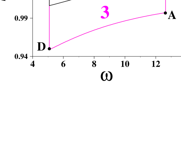
Figure 6: Three cycles corresponding to the minimal cycle time ”1”, zero power output ”2” and positive power output ”3”. The time allocations on the isochores are: on cycle ”1” $\tau_{h}=0.32$,  $\tau_{c}=0.64$,  on cycle ”2”: $\tau_{h}=0.581$,  $\tau_{c}=1.1602$,  and on cycle ”3”: $\tau_{h}=1.5$,  $\tau_{c}=3.6$.  The common parameter values on all three cycles are: $\tau_{ab}=0.05$,  $\tau_{ba}=0.06$, $J=2$, $\Gamma_{h}=1.0048$,  $\Gamma_{c}=0.10662$, $\omega_{b}=12.63545$, $\omega_{a}=5.0836387$, $T_{h}=7.5,~{}T_{c}=1.5$.

A search was carried out for time allocations where the cycle does not close, therefore no limit cycle exist. In general it was very difficult to find such conditions. These atypical cases with extremely small time allocations, were characterized by a non uniqueness of the limit cycle. For slightly longer time allocations a unique limit cycle was found which does not represent an engine. The reason is that the cooling on the cold isochore was not sufficient to dissipate the energy increase on the adiabats. As a result additional cooling was required on the hot isochore. The onset where heat is transfered by the engine from the hot to the cold bath was termed in the analogous engine based on a phenomenological description of friction Feldmann and Kosloff (2000), as the minimal cycle time (Cf. Cycle ”1” in fig. 6). Additional time allocation is required to reach the onset of positive work output (Cf. Cycle ”2” in fig. 6).

V.2.2 Entropy Production

The position of the limit cycle is determined by the balance of entropy. Since on the adiabatic branches the von Neumann entropy is constant the increase in the entropy of the working medium on the hot isochore should be exactly compensated on the cold isochore.

Examining the entropy changes on the hot isochore, one can compare the external entropy production $\Delta S^{ext}_{h}=-{\cal Q}_{h}/T_{h}$ to the internal change. Schlögl suggested Schlögl (1971); Feldmann et al. (1985), that the internal entropy production is related to the difference in the conditional entropy associated with the equilibrium state:

$$\Delta S^{E}_{h}~{}~{}=~{}~{}{\cal S}_{E}\left({\boldsymbol{\mathrm{\hat{\rho}}}}_{A}|{\boldsymbol{\mathrm{\hat{\rho}}}}_{eq}(T_{h})\right)-{\cal S}_{E}\left({\boldsymbol{\mathrm{\hat{\rho}}}}_{B}|{\boldsymbol{\mathrm{\hat{\rho}}}}_{eq}(T_{h})\right)~{}~{},$$ (54)

where ${\boldsymbol{\mathrm{\hat{\rho}}}}_{A}$ is the state at point $A$ on the beginning of the hot isochore, ${\boldsymbol{\mathrm{\hat{\rho}}}}_{B}$ is the state at point $B$ at the end of the hot isochore and ${\boldsymbol{\mathrm{\hat{\rho}}}}_{eq}(T_{h})$ is the equilibrium state at point $E$. Using the fact that the equilibrium density operator is diagonal in the energy representation i.e. ${\cal S}_{E}\left({\boldsymbol{\mathrm{\hat{\rho}}}}_{A}|{\boldsymbol{\mathrm{\hat{\rho}}}}_{eq}(T_{h})\right)={\cal S}_{E}({\boldsymbol{\mathrm{\hat{\rho}}}}_{A})-E_{A}/T_{h}+\log Z$, Eq. (54) takes the form:

$$\Delta S^{E}_{h}~{}~{}=~{}~{}{\cal S}_{E}\left({\boldsymbol{\mathrm{\hat{\rho}}}}_{A}\right)-{\cal S}_{E}\left({\boldsymbol{\mathrm{\hat{\rho}}}}_{B}\right)-\frac{{\cal Q}_{h}}{T_{h}}$$ (55)

since ${\cal Q}_{h}=(E_{b}-E_{a})$.

The full quantum characteristics representing the deviation of the density operator from the energy representation are obtained by the conditional entropy:

$$\Delta S^{u}_{h}~{}~{}=~{}~{}{\cal S}\left({\boldsymbol{\mathrm{\hat{\rho}}}}_{A}|{\boldsymbol{\mathrm{\hat{\rho}}}}_{eq}(T_{h})\right)-{\cal S}\left({\boldsymbol{\mathrm{\hat{\rho}}}}_{B}|{\boldsymbol{\mathrm{\hat{\rho}}}}_{eq}(T_{h})\right)~{}~{}=~{}~{}{\cal S}\left({\boldsymbol{\mathrm{\hat{\rho}}}}_{A}\right)-{\cal S}\left({\boldsymbol{\mathrm{\hat{\rho}}}}_{B}\right)-\frac{{\cal Q}_{h}}{T_{h}}~{}~{}.$$ (56)

For very long cycle times and sufficient time allocation on the isochores the system is diagonal in the energy representation. As a result Eq. (56) and Eq. (54) are equivalent. The difference between the internal entropy production $\Delta S^{u}_{h}$ and the external $\Delta S^{ext}_{h}=-{\cal Q}_{h}/T_{h}$ represents the entropy increase in the working medium. The same measures can be applied to the cold isochore. Summing the entropy changes on the two branches leads to equality between the changes in external and internal entropy production:

$$\Delta S^{u}_{h}+\Delta S^{u}_{c}~{}~{}=~{}~{}-\left(\frac{{\cal Q}_{h}}{T_{h}}~{}+~{}\frac{{\cal Q}_{c}}{T_{c}}\right)~{}~{},$$ (57)

since the von Neumann entropy ${\cal S}$ is constant on the adiabats. The energy entropy is not constant on the adiabats leading to a different relation for the energy entropy production:

$$\Delta S^{E}_{h}+\Delta S^{E}_{c}~{}~{}=~{}~{}-\left(\frac{{\cal Q}_{h}}{T_{h}}~{}+~{}\frac{{\cal Q}_{c}}{T_{c}}\right)+\Delta{\cal S}^{E}_{ba}+\Delta{\cal S}^{E}_{ab}~{}~{},$$ (58)

where $\Delta{\cal S}^{E}_{ab}$ is the change in energy entropy on the adiabat which can be interpreted as the entropy generation on the adiabats.

VI Conclusions

Summarizing the study is best carried out by addressing the questions raised in the introduction.

VI.1 How do the control parameters characterize the approach to the limit cycle?

The existence of a limit cycle is subject to there being a unique invariant of the global propagator. The invariant has an eigenvalue $\mu_{0}=1$ and its eigenvector is expressed via the expectation values of ${\boldsymbol{\mathrm{\hat{B}}}}_{1}$, ${\boldsymbol{\mathrm{\hat{B}}}}_{2}$ ${\boldsymbol{\mathrm{\hat{B}}}}_{3}$ and ${\boldsymbol{\mathrm{\hat{I}}}}$ in the limit cycle.

Quantum measures were developed to characterize the approach to the limit cycle: the conditional entropy and the quantum distance. These measures show a monotonic approach to the limit cycle. The projected measures such as the energy distance or energy conditional entropy can show an oscillatory approach to the limit cycle. Close to the limit cycle the rate of approach of all measures converge to the same value. The quantum distance was always larger than the probability distance associated with the measurement of energy. Dephasing eroded the deviation between the two distances.

Longitudinal and a transverse modes of approach to the limit cycle could be identified. The rate of approach is associated to the eigenvalues of the propagator. The eigenvalue $\mu_{1}$ determines the longitudinal relaxation rate. $\mu_{1}$ exponentially depends on the accumulated energy relaxation on the hot and cold isochores $\mu_{1}\propto e^{-(\Gamma_{h}\tau_{h}+\Gamma_{c}\tau_{c})}$. The transverse rate of approach is associated with the eigenvalues $\mu_{2/3}$. Their magnitude depends on the accumulated dephasing on the hot and cold isochores $|\mu_{2/3}|\propto e^{-\left((\Gamma_{h}+\gamma_{h}\Omega_{h}^{2})\tau_{h}+(\Gamma_{c}+\gamma_{c}\Omega_{c}^{2})\tau_{c}\right)}$. The phase $\phi$ of $\mu_{2/3}$ is linear in the time allocation $\tau_{ab}+\tau_{ba}$. The dependence of the rate of relaxation on other parameters such as $J$ was found to be weak.

VI.2 Can conditions be found for non-existence of the limit cycle?

When no time is allocated to the hot and cold isochores $\tau_{h}=\tau_{c}=0$ then the evolution is unitary and the modulus of all eigenvalues of the propagator become 1. As a result no unique limit cycle can be found. For very short times allocated to the isochores, two eigenvalues of the cycle propagator became equal to one, again no limit cycle is obtained in these conditions. Therefore there exist a $\delta\tau\ll 1$ range of time allocation on the isochores for which no unique limit cycle can be closed.

VI.3 What are the irreversible properties of the limit cycle?

Heat transport between the working medium and the baths is a common source of irreversibility for all realistic heat engines. If this is the only source of entropy generation the engine is classified as endoreversible Curzon and Ahlborn (1975); P. Salamon, J.D. Nulton, G. Siragusa, T.R. Andersen and A. Limon (2001), meaning that entropy is only generated on the interface and that the internal operation is reversible. The dissipative forces accompanying heat transfer were found to be sufficient to drive a quantum two-level endoreversible heat engine to a limit cycle T. Feldmann and Salamon (1996).

Friction is an additional source of irreversibility for all realistic heat engines, characterized by an internal entropy production. The heat generated by friction eventually has to be disposed in the cold bath. The performance of the present first principle quantum engine has been shown to be limited by a friction like phenomena Feldmann and Kosloff (2000). The key to the understanding of the quantum origin of friction lies in the difference between the energy entropy ${\cal S}_{E}$ and the von Neumann entropy ${\cal S}$. Since the von Neumann entropy is constant on the adiabats one could classify the model as endoreversible (Cf. Eq. (57)). Following the engines cycle by observing its energy changes shows characteristics of entropy generation on the adiabats (Cf. Eq. (58)).

The most illuminating case which characterizes the irreversible character due to the nonadiabatic dynamics is a cycle composed of two adiabats and only a cold isochore as displayed in Fig. 5. External work is converted to internal heat which is dissipated to the cold bath. The only phenomena that fits this behavior is friction. Surprisingly, the von Neumann entropy for the complete cycle trajectory is constant. This is in contrast to a power producing cycle where the von Neumann entropy changes on the isochores. A detailed analysis of the von Neumann entropy change on the cold isochore performed in the energy representation unravel the picture. A decrease in the entropy of diagonal elements, equivalent to $\Delta{\cal S}_{E}$ due to cooling of the working medium is exactly compensated by an entropy increase due to dephasing i.e. loss of the nondiagonal elements. It seems therefore that friction is the result of the interplay between the unitary evolution on the adiabats and the dissipative dynamics on the cold isochore. Friction is found only when the state of the quantum engine deviates from a diagonal energy representation. Such dynamics are a consequence of the nonadiabatic operation conditions caused by the noncommutability of the working medium Hamiltonian at different points along the cycle trajectory. These observations are the basis for a quantum control of friction which will be presented in a future study.

Appendix A Analytical solution of the propagator on the adiabats

The analytic solution for the propagator on the adiabats is based on the Lie group structure of the $\{\bf\hat{B}\}$ operators. The unitary evolution operator $\bf\hat{U}(t)$ for an explicitly time dependent Hamiltonians is obtained from the Schrödinger equation:

$$-i\frac{d}{dt}{{\bf\hat{U}}(t)}~{}=~{}{\bf\hat{H}}(t){\bf\hat{U}}(t),~{}~{}~{}~{}~{}~{}~{}~{}{\bf\hat{U}}(0)={\bf\hat{I}}~{}~{}~{}.$$ (59)

The propagated set of operators becomes:

$${\vec{\bf\hat{B}}}(t)~{}=~{}{\bf\hat{U}}(t)\vec{\bf\hat{B}}(0){\bf\hat{U}}^{\dagger}(t)~{}=~{}{\cal U}_{a}(t){\vec{\bf\hat{B}}}(0)~{}~{}~{},$$ (60)

and is related to the super-evolution operator ${\cal U}_{a}(t)$. Based on the group structure Wei and Norman, Wei and Norman (1963) constructed a solution to Eq. (59) for any operator ${\bf\hat{H}}$ which can be written as a linear combination of the operators in the closed Lie algebra ${\bf\hat{H}}(t)~{}=~{}\sum_{j=1}^{m}h_{j}(t){\bf\hat{B}}_{i}$, where the $h_{i}(t)$ are scalar functions of $t$. In such a case the unitary evolution operator ${\bf\hat{U}}(t)$ can be represented in the product form:

$${\bf\hat{U}}(t)~{}=~{}\prod_{k=1}^{m}\exp(\alpha_{k}(t){\bf\hat{B}}_{k})~{}~{}~{}.$$ (61)

The product form Eq. (61) substitutes the time dependent operator equation (59) with a set of scalar differential equations for the functions $\alpha_{k}(t)$. Writing the unitary evolution operator explicitly leads to:

$${\bf\hat{U}}(t)~{}=~{}\exp(i\frac{\alpha_{1}(t)}{\sqrt{2}}{\bf\hat{B}_{1}})\exp(i\frac{\alpha_{2}(t)}{\sqrt{2}}{\bf\hat{B}_{2}})\exp(i\frac{\alpha_{3}(t)}{\sqrt{2}}{\bf\hat{B}_{3}})$$ (62)

The $\sqrt{2}$ factor is introduced for technical reasons. Based on the group structure Wei and Norman (1963) Eq. (59) leads to the following set of differential equations for the coefficients $\alpha$:

$$\dot{\alpha}_{1}=\sqrt{2}\omega(t)+\sqrt{2}J(\frac{\sin(\alpha_{1})\sin(\alpha_{2})}{\cos(\alpha_{2})})~{};~{}~{}\dot{\alpha}_{2}=\sqrt{2}J\cos(\alpha_{1})~{};~{}~{}\dot{\alpha}_{3}=\frac{\sqrt{2}J\sin(\alpha_{1})}{\cos(\alpha_{2})}~{}~{}~{}.$$ (63)

Appendix B The Density Operators

B.1 Functions of the Density Operators

B.1.1 Computation of ${\boldsymbol{\mathrm{\hat{\rho}}}}_{p}^{\frac{1}{2}}$ and $\log{\boldsymbol{\mathrm{\hat{\rho}}}}_{p}$

First ${\boldsymbol{\mathrm{\hat{\rho}}}}_{p}$, Eq. (42), is diagonalized by the unitary matrices ${Q_{p}}~{},~{}Q^{\dagger}_{p}$:

$$\begin{array}[]{c}{Q_{p}}\end{array}~{}~{}=~{}\left(\begin{array}[]{cccc}-\frac{(b_{2}+ib_{3})}{\sqrt{2D(D+b_{1})}}&0&0&\sqrt{\frac{(D+b_{1})}{2D}}\\ 0&1&0&0\\ 0&0&1&0\\ \frac{(b_{2}+ib_{3})}{\sqrt{2D(D-b_{1})}}&0&0&\sqrt{\frac{(D-b_{1})}{2D}}\\ \end{array}\right)~{}~{},$$ (69)

leading to:

$$Q_{p}{\boldsymbol{\mathrm{\hat{\rho}}}}_{p}Q^{\dagger}~{}=~{}\left(\begin{array}[]{cccc}\frac{1}{4}-\frac{D}{\sqrt{2}}+\frac{b_{5}}{2}&0&0&0\\ 0&\frac{1}{4}+\frac{b_{4}}{\sqrt{2}}-\frac{b_{5}}{2}&0&0\\ 0&0&\frac{1}{4}-\frac{b_{4}}{\sqrt{2}}-\frac{b_{5}}{2}&0\\ 0&0&0&\frac{1}{4}+\frac{D}{\sqrt{2}}+\frac{b_{5}}{2}\\ \end{array}\right)~{}=~{}{\boldsymbol{\mathrm{\hat{\rho}}}}_{vn}$$ (74)

where $D~{}=~{}\sqrt{b_{1}^{2}+b_{2}^{2}+b_{3}^{2}}$, and $\lambda_{i}$ are the eigenvalues of ${\boldsymbol{\mathrm{\hat{\rho}}}}$ which are the von Neumann probabilities, Cf. Eq. (47).

The eigenvalues of ${{\boldsymbol{\mathrm{\hat{\rho}}}}^{\frac{1}{2}}}$ become $\lambda_{1}^{\frac{1}{2}}$, $\lambda_{2}^{\frac{1}{2}}$, $\lambda_{3}^{\frac{1}{2}}$, $\lambda_{4}^{\frac{1}{2}}$. From Eq. 74 one has:   ${\boldsymbol{\mathrm{\hat{\rho}}}}_{p}~{}=~{}Q^{\dagger}_{p}{\boldsymbol{\mathrm{\hat{\rho}}}}_{vn}Q_{p}$,   therefore ${\boldsymbol{\mathrm{\hat{\rho}}}}_{p}^{\frac{1}{2}}~{}=~{}Q^{\dagger}_{p}{\boldsymbol{\mathrm{\hat{\rho}}}}_{vn}^{\frac{1}{2}}Q_{p}$, and $\log{\boldsymbol{\mathrm{\hat{\rho}}}}_{p}~{}=~{}Q^{\dagger}_{p}\log{\boldsymbol{\mathrm{\hat{\rho}}}}_{vn}Q_{p}$. Explicitly:

$$\begin{array}[]{c}{{\boldsymbol{\mathrm{\hat{\rho}}}}_{p}^{\frac{1}{2}}}\end{array}~{}~{}=~{}~{}\left(\begin{array}[]{cccc}\frac{\lambda_{4}^{\frac{1}{2}}+\lambda_{1}^{\frac{1}{2}}}{2}+\frac{b_{1}(\lambda_{4}^{\frac{1}{2}}-\lambda_{1}^{\frac{1}{2}})}{2D}&0&0&\frac{(b_{2}-ib_{3})(\lambda_{4}^{\frac{1}{2}}-\lambda_{1}^{\frac{1}{2}})}{2D}\\ 0&\lambda_{2}^{\frac{1}{2}}&0&0\\ 0&0&\lambda_{3}^{\frac{1}{2}}&0\\ \frac{(b_{2}+ib_{3})(\lambda_{4}^{\frac{1}{2}}-\lambda_{1}^{\frac{1}{2}})}{2D}&0&0&\frac{\lambda_{4}^{\frac{1}{2}}+\lambda_{1}^{\frac{1}{2}}}{2}-\frac{b_{1}(\lambda_{4}^{\frac{1}{2}}-\lambda_{1}^{\frac{1}{2}})}{2D}\\ \end{array}\right)$$ (80)

and

$$\begin{array}[]{c}{\log{\boldsymbol{\mathrm{\hat{\rho}}}}_{p}}\end{array}~{}~{}=~{}~{}\left(\begin{array}[]{cccc}\frac{\log\lambda_{4}+\log\lambda_{1}}{2}+\frac{b_{1}(\log\lambda_{4}-\log\lambda_{1})}{2D}&0&0&\frac{(b_{2}-ib_{3})(\log\lambda_{4}-\log\lambda_{1})}{2D}\\ 0&\log\lambda_{2}&0&0\\ 0&0&\log\lambda_{3}&0\\ \frac{(b_{2}+ib_{3})(\log\lambda_{4}-\log\lambda_{1})}{2D}&0&0&\frac{\log\lambda_{4}+\log\lambda_{1}}{2}-\frac{b_{1}(\log\lambda_{4}-\log\lambda_{1})}{2D}\\ \end{array}\right)$$ (86)

B.1.2 Computation of ${\boldsymbol{\mathrm{\hat{\rho}}}}_{e}^{\frac{1}{2}}$ and $\log{\boldsymbol{\mathrm{\hat{\rho}}}}_{e}$

To get ${\boldsymbol{\mathrm{\hat{\rho}}}}$ in the energy picture ${\boldsymbol{\mathrm{\hat{\rho}}}}_{p}$ is transformed by the matrix ${\cal C}$ which diagonalized the Hamiltonian, see Feldmann and Kosloff (2003). Denoting $\Omega=\sqrt{\omega^{2}+J^{2}}$,  $\mu=\sqrt{\frac{\Omega-\omega}{2\Omega}}$,  and $\chi=\sqrt{\frac{\Omega+\omega}{2\Omega}}$,    $\cal C$ becomes Feldmann and Kosloff (2003):

$$\begin{array}[]{c}{\cal C}\end{array}~{}~{}=~{}\left(\begin{array}[]{cccc}-\mu&0&0&\chi\\ 0&1&0&0\\ 0&0&1&0\\ \chi&0&0&\mu\\ \end{array}\right)$$ (92)

Observing, that ${\cal C}{\cal C}~{}=~{}I$, leads to: ${{\boldsymbol{\mathrm{\hat{\rho}}}}_{e}}={\cal C}{{\boldsymbol{\mathrm{\hat{\rho}}}}_{p}}{\cal C}$,

$$\begin{array}[]{c}{\boldsymbol{\mathrm{\hat{\rho}}}}_{e}\end{array}~{}~{}=~{}~{}~{}\left(\begin{array}[]{cccc}\frac{1}{4}-\frac{E}{\Omega\sqrt{2}}+\frac{b_{5}}{2}&0&0&+\frac{ib_{3}}{\sqrt{2}}-\frac{Jb_{1}}{\Omega\sqrt{2}}+\frac{\omega b_{2}}{\Omega\sqrt{2}}\\ 0&\frac{1}{4}+\frac{b_{4}}{\sqrt{2}}-\frac{b_{5}}{2}&0&0\\ 0&0&\frac{1}{4}-\frac{b_{4}}{\sqrt{2}}-\frac{b_{5}}{2}&0\\ -\frac{ib_{3}}{\sqrt{2}}-\frac{Jb_{1}}{\Omega\sqrt{2}}+\frac{\omega b_{2}}{\Omega\sqrt{2}}&0&0&\frac{1}{4}+\frac{E}{\Omega\sqrt{2}}+\frac{b_{5}}{2}\\ \end{array}\right)~{}~{}~{},$$ (98)

where $E=\omega b_{1}+Jb_{2}$. In equilibrium, the off-diagonal elements vanish.

${{\boldsymbol{\mathrm{\hat{\rho}}}}_{p}}={\cal C}{{\boldsymbol{\mathrm{\hat{\rho}}}}_{e}}{\cal C}$ , therefore  : ${{\boldsymbol{\mathrm{\hat{\rho}}}}_{vn}}=Q_{p}{{\boldsymbol{\mathrm{\hat{\rho}}}}_{p}}Q^{\dagger}_{p}=Q_{p}{\cal C}{{\boldsymbol{\mathrm{\hat{\rho}}}}_{e}}{\cal C}Q^{\dagger}_{p}$. It follows, that the diagonalizing matrices of ${\boldsymbol{\mathrm{\hat{\rho}}}}_{e}$, become:  $Q_{e}=~{}Q_{p}{\cal C}$,  and   $Q^{\dagger}_{e}~{}=~{}{\cal C}Q^{\dagger}_{p}$. As a result   ${\boldsymbol{\mathrm{\hat{\rho}}}}_{e}^{\frac{1}{2}}=Q^{\dagger}_{e}{{\boldsymbol{\mathrm{\hat{\rho}}}}_{vn}^{\frac{1}{2}}}Q_{e}$   and    $\log({\rho_{e}})=Q^{\dagger}_{e}\log({{\boldsymbol{\mathrm{\hat{\rho}}}}_{vn}})Q_{e}$. Explicitly:

$$\begin{array}[]{c}{{\boldsymbol{\mathrm{\hat{\rho}}}}_{e}^{\frac{1}{2}}}\end{array}~{}~{}=~{}~{}~{}\left(\begin{array}[]{cccc}\frac{\lambda_{4}^{\frac{1}{2}}+\lambda_{1}^{\frac{1}{2}}}{2}-\frac{E(\lambda_{4}^{\frac{1}{2}}-\lambda_{1}^{\frac{1}{2}})}{2D\Omega}&0&0&-\frac{(\lambda_{4}^{\frac{1}{2}}-\lambda_{1}^{\frac{1}{2}})\left(\omega b_{2}-Jb_{1}+i\Omega b_{3}\right)}{2D\Omega}\\ 0&\lambda_{2}^{\frac{1}{2}}&0&0\\ 0&0&\lambda_{3}^{\frac{1}{2}}&0\\ -\frac{(\lambda_{4}^{\frac{1}{2}}-\lambda_{1}^{\frac{1}{2}})\left(\omega b_{2}-Jb_{1}-i\Omega b_{3}\right)}{2D\Omega}&0&0&\frac{\lambda_{4}^{\frac{1}{2}}+\lambda_{1}^{\frac{1}{2}}}{2}+\frac{E(\lambda_{4}^{\frac{1}{2}}-\lambda_{1}^{\frac{1}{2}})}{2D\Omega}\\ \end{array}\right)~{}~{}~{}.$$ (104)

and

$$\begin{array}[]{c}{\log{\boldsymbol{\mathrm{\hat{\rho}}}}_{e}}\end{array}~{}~{}=~{}~{}~{}\left(\begin{array}[]{cccc}\frac{\log\lambda_{4}+\log\lambda_{1}}{2}-\frac{E(\log\lambda_{4}-\log\lambda_{1})}{2D\Omega}&0&0&-\frac{(\log\lambda_{4}-\log\lambda_{1})\left(\omega b_{2}-Jb_{1}+i\Omega b_{3}\right)}{2D\Omega}\\ 0&\log\lambda_{2}&0&0\\ 0&0&\log\lambda_{3}&0\\ -\frac{(\log\lambda_{4}-\log\lambda_{1})\left(\omega b_{2}-Jb_{1}-i\Omega b_{3}\right)}{2D\Omega}&0&0&\frac{\log\lambda_{4}+\log\lambda_{1}}{2}+\frac{E(\log\lambda_{4}-\log\lambda_{1})}{2D\Omega}\\ \end{array}\right)~{}~{}~{}.$$ (110)

Any function of the density matrix can be computed by the diagonalizing vectors of the density matrix.

B.2 Additional details of quantum distance

In subsection V.1, a closed form expression was obtained for the quantum distance, Eq. (48). For the computation the polarization frame, ${\boldsymbol{\mathrm{\hat{\rho}}}}_{p}$, was used.

The operator ${{\boldsymbol{\mathrm{\hat{M}}}}}=({\boldsymbol{\mathrm{\hat{\rho}}}})^{\frac{1}{2}}{\boldsymbol{\mathrm{\hat{\rho}}}}_{ref}({\boldsymbol{\mathrm{\hat{\rho}}}})^{\frac{1}{2}}$ required in Eq. (15) is first computed.

$$\begin{array}[]{c}{{\boldsymbol{\mathrm{\hat{M}}}}}\end{array}~{}~{}=~{}~{}$$ (112)

$$\left(\begin{array}[]{cccc}Q+\frac{b_{1}(n)}{\sqrt{2}}(Y+x_{n})&0&0&(\frac{b_{2}(n)}{\sqrt{2}}-i\frac{b_{3}(n)}{\sqrt{2}})Y+(\frac{b_{2}(lc)}{\sqrt{2}}-i\frac{b_{3}(lc)}{\sqrt{2}})x_{n}\\ 0&\Lambda_{2}&0&0\\ 0&0&\Lambda_{3}&0\\ (\frac{b_{2}(n)}{\sqrt{2}}+i\frac{b_{3}(n)}{\sqrt{2}})Y+(\frac{b_{2}(lc)}{\sqrt{2}}+i\frac{b_{3}(lc)}{\sqrt{2}})x_{n}&0&0&Q-\frac{b_{1}(n)}{\sqrt{2}}(Y+x_{n})\\ \end{array}\right)$$ (117)

where the notations of Eqs. (48) was used, (49)  and (50), and where
$\Lambda_{2}=\lambda_{2}^{\frac{1}{2}}(n)\lambda_{2}^{\frac{1}{2}}(lc)$, and  $\Lambda_{3}=\lambda_{3}^{\frac{1}{2}}(n)\lambda_{3}^{\frac{1}{2}}(lc)$.

Calculation of ${\cal D}({\boldsymbol{\mathrm{\hat{\rho}}}}_{n},{\boldsymbol{\mathrm{\hat{\rho}}}}_{lc})$,  requires the value of $tr\{\sqrt{{\boldsymbol{\mathrm{\hat{M}}}}}\}$. The matrix representation of ${{\boldsymbol{\mathrm{\hat{M}}}}}$ breaks up into two internal and external 2x2 sub-matrices. Denoting the eigenvalues of the external ${{\boldsymbol{\mathrm{\hat{M}}}}}_{1,4}$ submatrix by $\zeta_{i}$, one has:

$$\zeta_{1,4}~{}=~{}Q\pm\sqrt{\left(\frac{YD_{n}}{\sqrt{2}}\right)^{2}+\left(\frac{x_{n}D_{lc}}{\sqrt{2}}\right)^{2}+2x_{n}qY}$$ (118)

References

- Alicki and Lendi (1987) R. Alicki and K. Lendi, Quantum Dynamical Semigroups and Applications (Springer-Verlag, Berlin, 1987).
- Lindblad (1976) G. Lindblad, Comm. Math. Phys. 48, 119 (1976).
- Kraus (1971) K. Kraus, Appl.Phys. 64, 311 (1971).
- Geva and Kosloff (1992) E. Geva and R. Kosloff, J. Chem. Phys. 96, 3054 (1992).
- T. Feldmann and Salamon (1996) R. K. T. Feldmann, E. Geva and P. Salamon, Am. J. Phys. 64, 485 (1996).
- Feldmann and Kosloff (2000) T. Feldmann and R. Kosloff, Phys. Rev. E 61, 4774 (2000).
- Kosloff and Feldmann (2002) R. Kosloff and T. Feldmann, Phys. Rev. E 65, 055102 (2002).
- Feldmann and Kosloff (2003) T. Feldmann and R. Kosloff, Phys. Rev. E 68, 016101 (2003).
- Ruskai (2002) M. B. Ruskai, J. Math. Phys. 43, 4358 (2002).
- Vedral (2002) V. Vedral, Rev. Mod. Phys. 74, 197 (2002).
- Lindblad (1975) G. Lindblad, Comm. Math. Phys. 40, 147 (1975).
- Frigerio (1977) A. Frigerio, Lett. Math. Phys. 2, 79 (1977).
- Frigerio (1978) A. Frigerio, Comm. Math. Phys. 63, 269 (1978).
- Wootters (1981) W. Wootters, Phys. Rev. D 23, 357 (1981).
- Fischer (1922) R. A. Fischer, Proc. R. Soc. Edinbourgh 42, 321 (1922).
- Braunstein and Caves (1994) S. L. Braunstein and C. M. Caves, Phys.Rev.Lett. 72, 3439 (1994).
- Hübner (1992) M. Hübner, Physics Letters A 163, 239 (1992).
- Diósi and Salamon (1999) L. Diósi and P. Salamon, Part III, Energy in geometrical thermodynamics (edited by S.Sieniutycz and A. De Vos, 1999).
- Wei and Norman (1963) J. Wei and E. Norman, Proc. Am. Math. Soc. 15, 327 (1963).
- Schlögl (1971) F. Schlögl, Z. Phys. 249, 1 (1971).
- Feldmann et al. (1985) T. Feldmann, B. Andresen, A. Qi, , and P. Salamon, J. Chem. Phys. 83, 5849 (1985).
- Curzon and Ahlborn (1975) F. Curzon and B. Ahlborn, Am. J. Phys. 43, 22 (1975).
- P. Salamon, J.D. Nulton, G. Siragusa, T.R. Andersen and A. Limon (2001) P. Salamon, J.D. Nulton, G. Siragusa, T.R. Andersen and A. Limon, Energy 26, 307 (2001).