Two-mode entanglement in two-component Bose-Einstein condensates

Abstract

We study the generation of two-mode entanglement in a two-component Bose-Einstein condensate trapped in a double-well potential. By applying the Holstein-Primakoff transformation, we show that the problem is exactly solvable as long as the number of excitations due to atom-atom interactions remains low. In particular, the condensate constitutes a symmetric Gaussian system, thereby enabling its entanglement of formation to be measured directly by the fluctuations in the quadratures of the two constituent components [Giedke et al., Phys. Rev. Lett. 91, 107901 (2003)]. We discover that significant two-mode squeezing occurs in the condensate if the interspecies interaction is sufficiently strong, which leads to strong entanglement between the two components.

I introduction

Soon after the experimental realization of Bose-Einstein condensates (BECs), rich physical phenomena have been observed and predicted as well expt ; review ; Leggett . In particular, there has been a surge of interest in the quantum tunneling dynamics of BECs trapped in multiple wells, and much attention has been focused on Josephson effect in such systems review ; Leggett ; tunnel . On the other hand, it was shown that multi-particle entanglement can be generated in BECs via the coherent interactions between the atoms multi , and thereafter BECs have played a prominent role in the field of quantum information. For example, both multi-particle entanglement (i.e. spin squeezing) and two-mode entanglement can be generated in a spin-1 condensate with three hyperfine sublevels duan ; You . In this case, two-mode entanglement, describing the inseparability between the two modes (respectively with spin projection $m=\pm 1$), can be used as quantum information protocols to facilitate quantum teleportation of continuous variables Zeilinger ; Popescu .

On the other hand, in addition to BECs with spin 0 and 1, BECs with two internal degrees of freedom, e.g. the $|F=1,m=-1\rangle$ and $|F=2,m=2\rangle$ sublevels of ⁸⁷Rb, are also achievable experimentally and are often termed as two-component condensates rubidium ; Hall , which give rise to novel features such as phase separation Ho and the cancellation of mean field energy shift Meystre . Such condensates can be viewed as collections of interacting spin-half particles and can consequently display multi-particle entanglement through the emergence of spin squeezing Law . Likewise, two different kinds of atoms (e.g. ⁴¹K and ⁸⁷Rb) can also form stable two-component BECs KRbBEC . More interestingly, the interspecies interaction of these two-component BECs can be varied by the application of magnetic control magint , thus hastening various experimental and theoretical investigations in this field.

Recently, there have been several discussions on the dynamics of a two-component condensate trapped in a double-well potential lobo ; Ng . The behaviors of such systems, which can be realized experimentally with the current technology, are arguably much richer than those of single-component condensates because of the interspecies interaction. For example, in a recent paper Ng we studied the tunneling dynamics of a two-component condensate whose two components are initially separated by the potential barrier between a double-well. We found that in the strong scattering regime atoms in the two components can tunnel through the barrier in a correlated manner Ng . As both the scattering strength and the tunneling strength between the wells can be tuned independently with various experimental techniques magint ; Greiner , it is expected that such phenomena will become observable in the near future.

In this paper, we consider a two-component condensate trapped in a double-well potential. Both components of the condensate are initially prepared in the ground state of the double well and hence are separable at time $t=0$. The objective of the present paper is to study and quantify the generation of two-mode entanglement in such a condensate. Two-mode entanglement is commonly attributed to the inseparability of the density matrix describing two systems, which can be found in various experimental situations and is very useful in the applications of quantum measurement and quantum information Zoller ; Simon ; Polzik . In fact, entanglement between two ensembles of atoms with spin has recently been achieved experimentally via interaction with polarized light Polzik , and the concept of two-mode entanglement has been generalized to describe such spin systems duan . Since each component of a two-component condensate in a double-well can be described as a collection of spin-half particles, with the two spatially localized modes in the two wells playing respectively the roles of spin-up and spin-down states, the condensate is in fact equivalent to two interacting gigantic spins that can be described in terms of continuous variables duan . While it has been shown that the intra-species interaction is able to create spin-squeezing for a single-component condensate trapped a double-well potential Law , in this paper we will demonstrate that the inter-species interaction is responsible for the generation of two-mode entanglement. It is the intriguing interplay of the inter-species and the intra-species interactions that sparks our investigation in such systems. By applying the Holstein-Primakoff transformation (HPT) HP , which reduces this two-spin system to two coupled oscillators, we show that our system is exactly solvable as long as the number of excitations due to atom-atom interactions remains low. More remarkably, the condensate in fact forms a symmetric Gaussian system. Therefore, we can directly evaluate the entanglement of formation (i.e. the von-Neumann entropy for a pure state) of the system from the fluctuations in the quadratures of the two constituent components duan ; Zoller ; Simon ; Giedke . In accordance with the schemes proposed recently by Duan et al. Zoller ; Simon and Giedke et al. Giedke , we define a two-mode entanglement parameter that measures the fluctuations in the quadratures and in turn analyze the degree of entanglement between the two components of the condensate in the present paper. Our discovery is that strong interspecies interaction can lead to significant two-mode squeezing in the condensate and hence strong entanglement between the two components.

The structure of our paper is as follows. In section II, we introduce the Hamiltonian of our system and classify it into symmetric and asymmetric cases according to the properties of the constituent condensates. In section III, we consider specifically a system with a large number of atoms. An effective Hamiltonian, which is exactly solvable, is then derived from the HPT. In section IV, we introduce the two-mode entanglement parameter duan ; Zoller ; Simon ; Giedke to describe and quantify the entanglement in our system. In section V, we study in detail the two-mode entanglement parameter for several typical cases. Finally, we discuss the physical meaning of the two-mode entanglement parameter in section VI and consider generalization our approach to mixed states.

II Tunneling two-component BEC

We first consider the tunneling dynamics of a two-component BEC trapped in a symmetric double-well potential. The total number of atoms in components $A$ and $B$ of the condensate are $N_{a}$ and $N_{b}$ respectively. We will further assume that the interaction between the atoms is sufficiently weak and adopt the two-mode approximation to describe the tunneling process. Under such approximation, the condensate dwelling in each potential minimum is adequately described by a single localized mode function walls ; raghavan ; juha . Considering the effect of quantum tunneling and the conservation of the particle number of each component, we obtain the Hamiltonian of the system:

$$H = \frac{\Omega_{a}}{2}({\hat{a}^{{\dagger}}_{L}}\hat{a}_{R}+{\hat{a}^{{\dagger}}_{R}}\hat{a}_{L})+\frac{\Omega_{b}}{2}({\hat{b}^{{\dagger}}_{L}}\hat{b}_{R}+{\hat{b}^{{\dagger}}_{R}}\hat{b}_{L})+{\kappa}({\hat{a}^{{\dagger}}_{L}}\hat{a}_{L}{\hat{b}^{{\dagger}}_{L}}\hat{b}_{L}+{\hat{a}^{{\dagger}}_{R}}\hat{a}_{R}{\hat{b}^{{\dagger}}_{R}}\hat{b}_{R})$$ (1)

$$+\frac{\kappa_{a}}{2}\left[({\hat{a}^{{\dagger}}_{L}}\hat{a}_{L})^{2}+({\hat{a}^{{\dagger}}_{R}}\hat{a}_{R})^{2}\right]+\frac{\kappa_{b}}{2}\left[({\hat{b}^{{\dagger}}_{L}}\hat{b}_{L})^{2}+({\hat{b}^{{\dagger}}_{R}}\hat{b}_{R})^{2}\right].$$

Here $\hat{a}^{{\dagger}}_{j}$ ($\hat{a}_{j}$) and $\hat{b}^{{\dagger}}_{j}$ ($\hat{b}_{j}$) are respectively the creation (annihilation) operators of components $A$ and $B$ residing in the $j$-th well, $j=L,R$. Since there are two spatial modes (the $L$ and $R$ modes) available for each component, the Hamiltonian above in fact consists of four bosonic operators. Besides, the parameters $\Omega_{a}$($\Omega_{b}$), $\kappa_{a}$($\kappa_{b}$) and $\kappa$ are the tunneling, intraspecies interaction strength of component $A$($B$) and the interspecies interaction strength respectively.

For the convenience of the subsequent discussion of two-mode entanglement, it is instructive to represent this Hamiltonian in terms of angular momentum operators by following through the standard Schwinger oscillator model to construct a set of spin operators for each component Schwinger :

$$\hat{J}_{\alpha{x}} = \frac{1}{2}({\hat{\alpha}^{{\dagger}}_{L}}\hat{\alpha}_{L}-{\hat{\alpha}^{{\dagger}}_{R}}\hat{\alpha}_{R}),$$

$$\hat{J}_{\alpha{y}} = \frac{1}{2i}({\hat{\alpha}^{{\dagger}}_{L}}\hat{\alpha}_{R}-{\hat{\alpha}^{{\dagger}}_{R}}\hat{\alpha}_{L}),$$ (2)

$$\hat{J}_{\alpha{z}} = \frac{1}{2}({\hat{\alpha}^{{\dagger}}_{L}}\hat{\alpha}_{R}+{\hat{\alpha}^{{\dagger}}_{R}}\hat{\alpha}_{L}),$$

where $\alpha=a,b$. Here ${\hat{\bf J}}_{\alpha}=(\hat{J}_{\alpha{x}},\hat{J}_{\alpha{y}},\hat{J}_{\alpha{z}})$ obey the usual angular momentum commutation relations. In the following we will denote the eigenstates of $\hat{J}^{2}_{\alpha}\equiv\hat{J}_{\alpha{x}}^{2}+\hat{J}_{\alpha{y}}^{2}+\hat{J}_{\alpha{z}}^{2}$ and $\hat{J}_{\alpha z}$ with $|j_{\alpha},m_{\alpha}\rangle$ such that $\hat{J}^{2}_{\alpha}|j_{\alpha},m_{\alpha}\rangle=j_{\alpha}(j_{\alpha}+1)|j_{\alpha},m_{\alpha}\rangle$, and $\hat{J}_{\alpha{z}}|j_{\alpha},m_{\alpha}\rangle=m_{\alpha}|j_{\alpha},m_{\alpha}\rangle$, where $j_{\alpha}=N_{\alpha}/2$. In terms of $\hat{{\bf J}}_{a}$ and $\hat{{\bf J}}_{b}$, the Hamiltonian (1) can be rewritten as

$$H = {\Omega_{a}}\hat{J}_{az}+{\Omega_{b}}\hat{J}_{bz}+\kappa_{a}\hat{J}^{2}_{ax}+\kappa_{b}\hat{J}^{2}_{bx}+2{\kappa}\hat{J}_{ax}\hat{J}_{bx}.$$ (3)

In the absence of atom-atom interactions, the ground state of the system is obviously given by the product state $|j_{a},-j_{a}{\rangle}|j_{b},-j_{b}{\rangle}$ and the two components are not entangled. In the following discussion we consider how the atom-atom interactions affect the evolution of the initial state

$$|\Psi(t=0)\rangle=|j_{a},-j_{a}{\rangle}|j_{b},-j_{b}{\rangle}\,,$$ (4)

and show that the two components will get entangled through the inter- and intra-species interactions.

To facilitate later discussion on the phenomenon of entanglement, we further classify two-component condensates according to the symmetry properties of the two components constituting the condensate. In a symmetric two-component BEC, the parameters of component $A$ and component $B$ are equal to one another, namely $\Omega_{a}=\Omega_{b}$ and $\kappa_{a}=\kappa_{b}$. These conditions hold approximately for condensates consisting of the hyperfine states $|F=1,m=-1\rangle$ and $|F=2,m=1\rangle$ of ⁸⁷Rb Hall . The two components of such condensates have essentially same masses and magnetic moments and hence $\Omega_{a}=\Omega_{b}$. Their intra-species scattering lengths are quite close and, in addition, $\kappa_{a}\approx\kappa_{b}\approx\kappa$ rubidium . In a quasi-identical two-component BEC where $\Omega_{a}=\Omega_{b}=\Omega$ and $\kappa_{a}=\kappa_{b}=\kappa$, the Hamiltonian (3) reduces to:

$$H_{1}={\Omega}\hat{J_{z}}+{\kappa}\hat{J^{2}_{x}}.$$ (5)

where $\hat{{\bf J}}=\hat{{\bf J}}_{a}+\hat{{\bf J}}_{b}$ is the total angular momentum of the system. Despite that the Hamiltonian of such a two-component condensate is identical to that of a single-component one Law , the distinguishability of the two species entails the study of two-mode entanglement.

Meanwhile, for asymmetric two-component BECs relevant physical parameters of the two components are generally different. For example, it has recently been observed in the experiment that the condensates of potassium and rubidium (Rb-K), which have different scattering lengths and masses, can form stable two-component condensates KRbBEC . Therefore, it is deemed appropriate to develop a generic analytical scheme to study such condensates. In the following discussion, we will make use of the HPT HP to carry out a thorough analytical investigation on the entanglement between the two constituent components.

III Bosonic operator approximation

In this section, we consider the evolution of a condensate with large numbers of atoms and sufficiently weak scattering strengths, namely $N_{a(b)}\gg 1$ and $\Omega_{a(b)}{\gg}\kappa_{a},\kappa_{b},\kappa$. As the initial state, given by (4), is the ground state of a non-interacting condensate and the scattering strengths are weak, only the low-lying states will be excited in the evolution and the coherence of tunneling process can be maintained. The current situation is in contradistinction to our previous study Ng that discovered correlated tunneling of the two components in the strong scattering regime. However, we will show that the inter-species interaction does lead to nontrivial entanglement of the two components.

To proceed, we apply the HPT to map angular momentum operators into bosonic operators HP ; Bosonization and show that under the HPT our system is in fact equivalent to two coupled harmonic oscillators. In HPT, the angular momentum operators

$$\hat{J}_{\alpha\pm}=\hat{J}_{\alpha x}\pm i\hat{J}_{\alpha y}\,,\quad\alpha=a,b\,,$$ (6)

and $\hat{J}_{\alpha{z}}$ are expressed in terms of bosonic operators $\hat{\alpha}$, $\hat{\alpha}^{{\dagger}}$:

$$\hat{J}_{\alpha{+}} = \hat{\alpha}^{{\dagger}}\sqrt{2j_{\alpha}-\hat{\alpha}^{{\dagger}}\hat{\alpha}},$$ (7)

$$\hat{J}_{\alpha{-}} = \left(\sqrt{2j_{\alpha}-\hat{\alpha}^{{\dagger}}\hat{\alpha}}\right)\hat{\alpha},$$ (8)

$$\hat{J}_{\alpha{z}} = (\hat{\alpha}^{{\dagger}}\hat{\alpha}-j_{\alpha}).$$ (9)

Here $\hat{\alpha}^{{\dagger}}$ and $\hat{\alpha}$ are standard bosonic operators satisfying $[\hat{\alpha},\hat{\alpha}^{{\dagger}}]=1$. Hence, the Hamiltonian (3) can be written as

$$H = \sum_{\alpha=a,b}\left[\Omega_{\alpha}({\hat{\alpha}^{\dagger}}\hat{\alpha}-j_{\alpha})+\frac{\kappa_{\alpha}{j_{\alpha}}}{2}\Bigg{(}\hat{\alpha}^{{\dagger}}\sqrt{1-\frac{\hat{\alpha}^{{\dagger}}\hat{\alpha}}{2j_{\alpha}}}+\sqrt{1-\frac{\hat{\alpha}^{{\dagger}}\hat{\alpha}}{2j_{\alpha}}}\hat{\alpha}\Bigg{)}^{2}\right]$$ (10)

$$+{\kappa\sqrt{j_{a}j_{b}}}\Bigg{(}\hat{a}^{{\dagger}}\sqrt{1-\frac{\hat{a}^{{\dagger}}\hat{a}}{2j_{a}}}+\sqrt{1-\frac{\hat{a}^{{\dagger}}\hat{a}}{2j_{a}}}\hat{a}\Bigg{)}\Bigg{(}\hat{b}^{{\dagger}}\sqrt{1-\frac{\hat{b}^{{\dagger}}\hat{b}}{2j_{b}}}+\sqrt{1-\frac{\hat{b}^{{\dagger}}\hat{b}}{2j_{b}}}\hat{b}\Bigg{)}.$$

Since $\Omega_{a(b)}\gg\kappa,\kappa_{a},\kappa_{b}$, it is arguable that

$$\frac{\langle{\hat{\alpha}^{{\dagger}}\hat{\alpha}}\rangle}{2j_{\alpha}}\ll 1,$$ (11)

leading to an approximate effective Hamiltonian,

$$H_{\rm eff}=\Omega_{a}{\hat{a}^{\dagger}{\hat{a}}}+\Omega_{b}{\hat{b}^{\dagger}{\hat{b}}}+\frac{1}{2}\Big{[}\kappa_{a}j_{a}(\hat{a}^{{\dagger}}+\hat{a})^{2}+\kappa_{b}j_{b}(\hat{b}^{{\dagger}}+\hat{b})^{2}+2\kappa\sqrt{j_{a}j_{b}}(\hat{a}^{{\dagger}}+\hat{a})(\hat{b}^{{\dagger}}+\hat{b})\Big{]}.$$ (12)

This Hamiltonian is analogous to that of two coupled oscillators and completely captures the essence of the dynamics of the two interacting BECs. Correspondingly, the initial state (4) is given by the vacuum state $|0_{a},0_{b}\rangle$ of the two decoupled oscillators described by the first two terms in $H_{\rm eff}$, where $|n_{a},n_{b}\rangle$ represents the Fock state of the oscillators.

To study the two-mode entanglement in the condensate, it is advantageous to make use of the position and the momentum operators:

$$\hat{q}_{a} = \frac{1}{\sqrt{2}}(\hat{a}^{{\dagger}}+\hat{a}),~{}~{}~{}~{}\hat{p}_{a}=i\frac{1}{\sqrt{2}}(\hat{a}^{{\dagger}}-\hat{a}),$$ (13)

$$\hat{q}_{b} = \frac{1}{\sqrt{2}}(\hat{b}^{{\dagger}}+\hat{b}),~{}~{}~{}~{}\hat{p}_{b}=i\frac{1}{\sqrt{2}}(\hat{b}^{{\dagger}}-\hat{b}),$$ (14)

and to rewrite the effective Hamiltonian as

$$H_{\rm eff}=\frac{\Omega_{a}}{2}(\hat{q}_{a}^{2}+\hat{p}^{2}_{a})+\frac{\Omega_{b}}{2}(\hat{q}_{b}^{2}+\hat{p}^{2}_{b})+\kappa_{a}j_{a}\hat{q}_{a}^{2}+\kappa_{b}j_{b}\hat{q}_{b}^{2}+2\kappa\sqrt{j_{a}j_{b}}\hat{q}_{a}\hat{q}_{b}.$$ (15)

It is then straightforward to solve the resulting equations of motion of $\hat{q}_{a}(t),\hat{p}_{a}(t),\hat{q}_{b}(t)$ and $\hat{p}_{b}(t)$. For convenience, we express the solutions in matrix form, which reads

$$X(t) \equiv (\hat{q}_{a}(t),\hat{p}_{a}(t),\hat{q}_{b}(t),\hat{p}_{b}(t))^{T}$$ (16)

$$= U(t)X(t=0).$$

Here $U(t)$ is a real $4\times{4}$ matrix representing the evolution operator and can be written as

$$U=\left(\begin{array}[]{clcr}C&E_{1}\\ E_{2}&D\end{array}\right),$$

with the $2\times{2}$ matrices $C$, $D$ and $E$ being explicitly given by

$$C=\frac{1}{(\mu_{2}-\mu_{1})}\left(\begin{array}[]{cc}\mu_{2}\cos\omega_{1}{t}-\mu_{1}\cos\omega_{2}{t}&\Omega_{a}(\mu_{2}\sin\omega_{1}{t}/\omega_{1}-\mu_{1}\sin\omega_{2}{t}/\omega_{2})\\ -(\omega_{1}\mu_{2}\sin\omega_{1}{t}-\omega_{2}\mu_{1}\sin\omega_{2}{t})/\Omega_{a}&\mu_{2}\cos\omega_{1}{t}-\mu_{1}\cos\omega_{2}{t}\end{array}\right),$$

$$D=\frac{1}{(\mu_{2}-\mu_{1})}\left(\begin{array}[]{cc}-\mu_{1}\cos\omega_{1}{t}+\mu_{2}\cos\omega_{2}{t}&-\Omega_{b}(\mu_{1}\sin\omega_{1}{t}/\omega_{1}-\mu_{2}\sin\omega_{2}{t}/\omega_{2})\\ (\mu_{1}\omega_{1}\sin\omega_{1}{t}-\mu_{2}\omega_{2}\sin\omega_{2}{t})/\Omega_{b}&-\mu_{1}\cos\omega_{1}{t}+\mu_{2}\cos\omega_{2}{t}\end{array}\right),$$

$$E_{1}=\frac{1}{(\mu_{2}-\mu_{1})}\left(\begin{array}[]{cc}-(\cos\omega_{1}{t}-\cos\omega_{2}{t})&-\Omega_{b}(\sin\omega_{1}{t}/\omega_{1}-\sin\omega_{2}{t}/\omega_{2})\\ (\omega_{1}\sin\omega_{1}{t}-\omega_{2}\sin\omega_{2}{t})/\Omega_{a}&-\Omega_{b}(\cos\omega_{1}{t}-\cos\omega_{2}{t})/\Omega_{a}\end{array}\right),$$

and

$$E_{2}=\frac{1}{(\mu_{2}-\mu_{1})}\left(\begin{array}[]{cc}-\Omega_{b}(\cos\omega_{1}{t}-\cos\omega_{2}{t})/\Omega_{a}&-\Omega_{b}(\sin\omega_{1}{t}/\omega_{1}-\sin\omega_{2}{t}/\omega_{2})\\ (\omega_{1}\sin\omega_{1}{t}-\omega_{2}\sin\omega_{2}{t})/\Omega_{a}&-(\cos\omega_{1}{t}-\cos\omega_{2}{t})\end{array}\right),$$

where

$$\mu_{1(2)} = \frac{\omega^{2}_{1(2)}-\Omega^{2}_{a}-2\kappa_{a}j_{a}\Omega_{a}}{2\kappa\Omega_{a}\sqrt{j_{a}j_{b}}},$$ (17)

and the normal mode frequencies of the coupled oscillation are

$$\omega_{1(2)} = \Bigg{\{}\left(\frac{\Omega^{2}_{a}+\Omega^{2}_{b}}{2}+\kappa_{a}j_{a}\Omega_{a}+\kappa_{b}j_{b}\Omega_{b}\right)$$ (18)

$$\pm\left[\left(\frac{\Omega^{2}_{a}-\Omega^{2}_{b}}{2}+\kappa_{a}j_{a}\Omega_{a}-\kappa_{b}j_{b}\Omega_{b}\right)^{2}+4\kappa^{2}j_{a}j_{b}\Omega_{a}\Omega_{b}\right]^{1/2}\Bigg{\}}^{1/2}.$$

This approximate solution, which is based on HPT, is valid as long as the condition (11) holds. However, if the normal frequency is complex, the system will become unstable. We can therefore determine the stability condition from (18):

$$|\kappa|<\frac{1}{2}\sqrt{\Bigg{(}\frac{\Omega_{a}}{j_{a}}+2\kappa_{a}\Bigg{)}\Bigg{(}\frac{\Omega_{b}}{j_{b}}+2\kappa_{b}\Bigg{)}}\equiv\kappa_{c}.$$ (19)

the HPT fails to yield a self-consistent solution for systems violating the inequality. It is interesting to note that in the limit where $j_{a},j_{b}\to\infty$, the condition for stability reduces to:

$$|\kappa|<\sqrt{\kappa_{a}\kappa_{b}}\equiv\kappa_{e},$$ (20)

which is a well known result for BECs in extended space, and violation of (20) will lead to the phase separation of two component BECs Ho ; phase-sep . It is also worthwhile to note that the stability criterion (19) depends on the numbers of atoms in the double-well and similar dependence has previously been found for two-component BECs in a single well phase-sep . We will, however, assume the stability criterion (19) is satisfied throughout the present study and obtain analytically the two-mode entanglement parameter for the condensate, which will be defined in the following section. We will see that in addition to yielding the analytic solution to the tunneling dynamics, the HPT performed here also facilitates our study on two-mode entanglement.

IV Theory of Two-mode Entanglement

Entanglement between two systems that are described in terms of continuous variables is usually indicated by an inequality in its Einstein-Podolsky-Rosen (EPR) uncertainty duan ; Zoller ; Simon :

$$\frac{1}{2}\left\{\langle[{\Delta}(\hat{q}_{a}+\hat{q}_{b})]^{2}\rangle+\langle[{\Delta}(\hat{p}_{a}-\hat{p}_{b})]^{2}\rangle\right\} < 1,$$ (21)

where $[\hat{q}_{m},\hat{p}_{n}]=i\delta_{mn}$ for $m,n=a,b$. $\hat{q}_{a(b)}$ and $\hat{p}_{a(b)}$ are respectively the position and momentum operators (or any pairs of quadratures) of system $a(b)$, and the above inequality simply implies that the positions (momenta) of the particles are strongly anti-correlated (correlated). In general, condition (21) is only a sufficient condition for entanglement and does not imply separability of the two systems even if it is violated duan ; Zoller . However, it has recently been shown that a necessary and sufficient condition for entanglement, which is analogous to (21), can be established if the combined system is a Gaussian one in the sense that if its Wigner characteristic function, defined by:

$$\chi^{(w)}(\lambda_{a},\lambda_{b}) = \text{tr}[{\rho}\text{exp}({\lambda_{a}}\hat{a}-{\lambda^{*}_{a}}\hat{a}^{{\dagger}}+{\lambda_{b}}\hat{b}-{\lambda^{*}_{b}}\hat{b}^{{\dagger}})]\,,$$ (22)

is a Gaussian function of $\lambda_{a}$ and $\lambda_{b}$ Zoller ; Giedke . Without loss of generality, one can assume that the expectation values of all quadratures vanish and hence the Wigner characteristic function of a Gaussian system is expressible as:

$$\chi^{(w)}(\lambda_{a},\lambda_{b}) = \text{exp}\Bigg{[}-\frac{1}{2}\Lambda^{T}M\Lambda\Bigg{]}\,\,,$$ (23)

where $M$ is a $4\times 4$ real symmetric matrix and the matrix $\Lambda$ is defined by $\Lambda\equiv(\lambda^{I}_{a},\lambda^{R}_{a},\lambda^{I}_{b},\lambda^{R}_{b})^{T}$. As the characteristic function can also be written as:

$$\chi^{(w)}(\lambda_{a},\lambda_{b}) = \text{tr}[{\rho}\text{exp}(i\sqrt{2}\Lambda^{T}X)]\,,$$ (24)

it is obvious that the matrix elements of $M$ are the correlation functions of the quadrature variables $X=(\hat{q}_{a},\hat{p}_{a},\hat{q}_{b},\hat{p}_{b})^{T}$. In fact, $M_{ij}=\langle(X_{i}X_{j}+X_{j}X_{i})\rangle$ and therefore $M$ is termed the covariance matrix.

As the amount of entanglement between the two systems is unaffected by local unitary operations, say local rotations in the $q$-$p$ plane and local squeezing operations, the matrix $M$ can be transformed into a standard form $M_{s}$ by several local operations Zoller :

$$M_{s}=\left(\begin{array}[]{clcr}n_{1}&0&c_{1}&0\\ 0&n_{2}&0&c_{2}\\ c_{1}&0&m_{1}&0\\ 0&c_{2}&0&m_{2}\end{array}\right),$$

where $n_{1},n_{2},m_{1},m_{2}$ are positive numbers, and

$$\frac{n_{1}-1}{m_{1}-1} = \frac{n_{2}-1}{m_{2}-1},$$ (25)

$$|c_{1}|-|c_{2}| = \sqrt{(n_{1}-1)(m_{1}-1)}-\sqrt{(n_{2}-1)(m_{2}-1)}.$$ (26)

It has recently been shown by Duan et al. that a Gaussian system is entangled if and only if the following inequality is satisfied Zoller ; Giedke :

$${a^{2}_{0}(n_{1}+n_{2})-2(|c_{1}|+|c_{2}|)+(m_{1}+m_{2})/{a^{2}_{0}}}<{2a^{2}_{0}+2/{a^{2}_{0}}},$$ (27)

where

$$a^{2}_{0} = \sqrt{\frac{m_{1}-1}{n_{1}-1}}=\sqrt{\frac{m_{2}-1}{n_{2}-1}}\,.$$ (28)

We therefore accordingly construct a two-mode entanglement parameter $\xi_{t}$Zoller ; Giedke :

$$\xi_{t}\equiv\frac{{a^{2}_{0}(n_{1}+n_{2})-2(|c_{1}|+|c_{2}|)+(m_{1}+m_{2})/{a^{2}_{0}}}}{{2a^{2}_{0}+2/{a^{2}_{0}}}}\,.$$ (29)

Physically speaking, $\xi_{t}>0$ is merely a suitably weighted EPR-type uncertainty in the squeezed quadratures of the system. The sufficient and condition for entanglement mentioned above can then be expressed in terms of an inequality involving this parameter:

$$\xi_{t}<1.$$ (30)

If, in addition, the system is a symmetric one such that $n_{1}=n_{2}=m_{1}=m_{2}$, Giedke et al. Giedke have recently shown that the parameter $\xi_{t}$ can also yield the entanglement of formation (EOF) of the system, $E_{F}$, Wooters :

$$E_{F}(\xi_{t}) = c_{+}(\xi_{t})\log[c_{+}(\xi_{t})]-c_{-}(\xi_{t})\log[c_{-}(\xi_{t})]\;\;{\rm if}\;0<\xi_{t}<1,$$ (31)

$$= 0\;\;{\rm otherwise,}$$

where the functions $c_{\pm}(z)$ are defined by $c_{\pm}(z)=[(z)^{-1/2}\pm(z)^{1/2}]^{2}/4$. It is noteworthy that EOF is a proper measure of the degree of entanglement between two systems and is equal to the von-Neumann entropy if the compound system remains in a pure state. However, unlike the von-Neumann entropy, EOF still works for mixed states. In fact, Josse et al. have recently measured the EOF of a pair of non-separable light beams with this scheme Josse . In the following section, we shall make use of the two-mode entanglement parameter $\xi_{t}$ to study how the two components of a BEC condensate trapped in double-well are entangled.

V Two-mode entanglement in BECs

To study two-mode entanglement in BECs, we first show that a two-component BEC indeed forms a Gaussian system. Since

$$\chi^{(w)}(\lambda_{a},\lambda_{b},t) = \text{tr}\left\{{\rho}\text{exp}\left[i\sqrt{2}\Lambda^{T}X(t)\right]\right\}$$ (32)

$$= \text{tr}\left\{{\rho}\text{exp}\left[i\sqrt{2}\left(U(t)^{T}\Lambda\right)^{T}X(t=0)\right]\right\}\,,$$

$\chi^{(w)}(\lambda_{a},\lambda_{b},t)$ can be obtained from $\chi^{(w)}(\lambda_{a},\lambda_{b},t=0)$ and we therefore consider the characteristic function at $t=0$. For the initial state $|0_{a},0_{b}\rangle$, it is readily shown that $\chi^{(w)}(\lambda_{a},\lambda_{b},t=0)$ is a Gaussian function and $M(t=0)$ is an identity matrix. $\chi^{(w)}(\lambda_{a},\lambda_{b},t)$ at other times can simply be obtained by the replacement $\Lambda\rightarrow U(t)\Lambda$. Consequently, we show that $\chi^{(w)}(\lambda_{a},\lambda_{b},t)$ is a Gaussian function of $\Lambda$ and:

$$\chi^{(w)}(\lambda_{a},\lambda_{b},t) = \text{exp}\left\{-\frac{1}{2}\left[U^{T}(t)\Lambda\right]^{T}M(0)U^{T}(t)\Lambda\right\}\,,$$ (33)

which directly yields the covariance matrix $M(t)$:

$$M(t) = U(t)M(0)U^{T}(t)$$ (34)

$$= U(t)U^{T}(t).$$

Hence, the condensate constitutes a Gaussian system to which the two-mode entanglement parameter applies.

After applying several local unitary transformations to $M(t)$, we obtain the matrix $M_{s}(t)$ of our system, which reads:

$$M_{s}(t)=\left(\begin{array}[]{clcr}n&0&c&0\\ 0&n&0&-c\\ c&0&n&0\\ 0&-c&0&n\end{array}\right).$$

Moreover, the matrix elements of the matrix $M_{s}$ are expressible in terms of the variances of the physical quantities as follows:

$$n = 2\left\{\langle{q^{2}_{a}}(t)\rangle\langle{p^{2}_{a}}(t)\rangle-[{\rm Re}\langle{q}_{a}(t){p}_{a}(t)\rangle]^{2}\right\}^{1/2}$$ (35)

$$= 2\left\{\langle{q^{2}_{b}}(t)\rangle\langle{p^{2}_{b}}(t)\rangle-[{\rm Re}\langle{q}_{b}(t){p}_{b}(t)\rangle]^{2}\right\}^{1/2},$$

$$c = 2\left[{\rm Re}(\langle{{q}_{a}(t){p}_{b}(t)}\rangle\langle{{q}_{b}(t){p}_{a}}(t)\rangle-\langle{q_{a}(t){q}_{b}(t)}\rangle\langle{p_{a}(t){p}_{b}(t)}\rangle)\right]^{1/2},$$ (36)

and the variances are given in the appendix for reference. It is then obvious that our system is a symmetric one with $n_{1}=n_{2}=m_{1}=m_{2}=n$ and hence $a_{0}=1$. Therefore, one can use the corresponding two-mode entanglement parameter, which is given by

$$\xi_{t} = n-c\,,$$ (37)

to evaluate the EOF of the system Giedke .

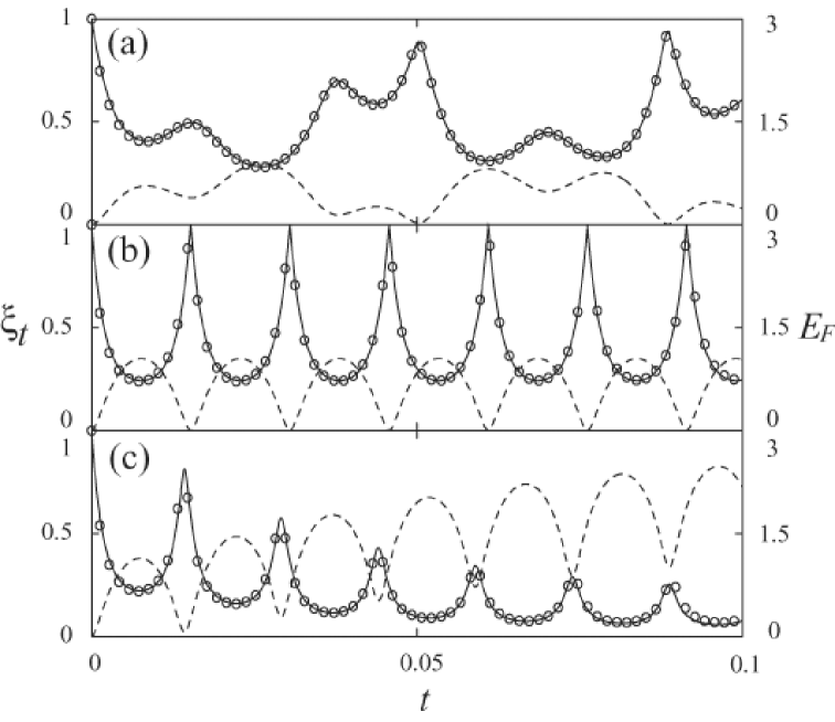
Figure 1: The time evolution of $\xi_{t}$ (solid line, left scale) and the EOF $E_{F}$ (dashed line, right scale) are shown for the symmetric case with $N_{a}=N_{b}=400$; $\kappa_{a}=\kappa_{b}=1$; $\Omega_{a}=\Omega_{b}=50$; and (a) $\kappa=0.50$; (b) $\kappa=1.00$; (c) $\kappa=1.12$. To gauge the accuracy of the HPT, the exact numerical solution of $\xi_{t}$ is shown by the empty circles.

Now we are ready to investigate the entanglement in our system with the help of $\xi_{t}$ and $E_{F}(\xi_{t})$. We first consider a quasi-identical two-component condensate (e.g. a Rb-Rb condensate), where $\kappa=\kappa_{a}=\kappa_{b}$ and $\Omega_{a}=\Omega_{b}=\Omega$. The time evolution of $\xi_{t}$ for such a condensate is shown in Fig. 1, where $N_{a}=N_{b}=400$, $\Omega_{a}=\Omega_{b}=50$, $\kappa_{a}=\kappa_{b}=1$ and $\kappa=0.50$ (Fig. 1(a)); $\kappa=1.00$ (Fig. 1(b)); $\kappa=1.12$ (Fig. 1(c)). Hereafter we adopt suitable units in which $\kappa_{b}=1$ for purpose of convenience. The solid line and empty circles are respectively results obtained from the HPT and numerical diagonalization of the original Hamiltonian, showing that the HPT indeed yields a good approximation in this regime. We also show the time evolution of the EOF, which equals the von-Neumann entropy in this case, by the dashed line in Fig. 1. It is obvious that our system is able to generate a substantial amount of two-mode entanglement for most of the time. Besides, one can see that there is a strong anti-correlation between these two curves, which can be understood as $E_{F}(\xi_{t})$ is a monotonically decreasing function of $\xi_{t}$ for $0\leq\xi_{t}\leq 1$.

It is remarkable that the degree of entanglement depends crucially on the inter-species interaction. Of course, it is obvious that the EOF or the entropy is zero when the interspecies interaction $\kappa$ vanishes. As shown in Fig. 1(a), (b) and (c), the entanglement parameter $\xi_{t}$ decreases while the EOF increases with increasing $\kappa$. Therefore, one can achieve optimal squeezing by properly controlling the interaction parameters. Besides, it is worthy of remark that in Fig. 1(c) $\kappa_{c}>\kappa>\kappa_{e}$. Therefore, the system is still a stable one and the HPT remains valid. Physically speaking, the availability of the two spatially separated modes in fact stabilizes the condensate despite that $\kappa>\kappa_{e}$ phase-sep .

We now switch our attention to asymmetric BECs consisting of two components with different physical characteristics. In fact, stable BECs of rubidium and potassium have recently been achieved in experiments and it is also possible to control the strength of interspecies interaction between the two components with a magnetic field magint . It is therefore deemed appropriate to investigate how the entanglement in such condensates changes with the interspecies interaction strength, $\kappa$. In the following, we assume that the tunneling strengths and the intraspecies interaction strengths of the two species are in the ratios of 1:1.45 and 1:1.33 respectively, which are reasonable estimates of experimental data for a Rb-K condensate walls .

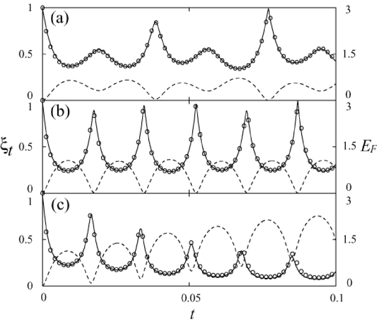
Figure 2: The time evolution of $\xi_{t}$ (solid line, left scale) and the EOF $E_{F}$ (dashed line, right scale) are shown for the asymmetric case with $N_{a}=N_{b}=400$; $\kappa_{a}=0.75$, $\kappa_{b}=1$; $\Omega_{a}=34.5$, $\Omega_{b}=50$; and (a) $\kappa=0.50$; (b) $\kappa=0.875$; (c) $\kappa=0.965$. To gauge the accuracy of the HPT, the exact numerical solution of $\xi_{t}$ is shown by the empty circles.

The two-mode entanglement parameters for three asymmetric cases with $\kappa=0.5,0.875,0.965$ are respectively shown in Fig. 2(a), (b) and (c). Considering the interspecies interaction $\kappa$ as an adjustable parameter, we find that a smaller $\xi_{t}$ (i.e., higher entanglement) can be obtained as the system becomes closer to the point of stability limit given by (19). As shown in Fig. 2(c), if $\kappa$ is increased and approaches the stability limit given by (19) from below, the two-mode entanglement parameter (the EOF) can attain much smaller (greater) values. Thus, the significance of the strength of interspecies interaction in two-mode entanglement generation is clearly demonstrated.

From the results illustrated in Figs. 1 and 2 it is manifest that a substantial increase of entanglement can be achieved in the vicinity of the stability limit (19). In fact, this novel feature can be understood heuristically as follows. In general, position (momentum) squeezed states of a harmonic oscillator can be produced by strengthening (weakening) its spring constant Scully . The two-component condensates can be viewed as a coupled oscillators and at the critical point of stability the eigenfrequenices are $(\Omega^{2}_{a}+\Omega^{2}_{b}+2\kappa_{a}j_{a}\Omega_{a}+2\kappa_{b}j_{a}\Omega_{b})^{1/2}$ and zero. As one of these frequencies, $\omega_{2}=0$, is markedly different from those in the interaction free case, the effect of squeezing in the position space and the momentum space is much pronounced in the vicinity of the critical point.

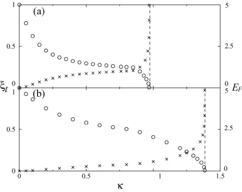
Figure 3: The maximal achievable values of $\xi_{t}$ (empty circles, left scale) and the EOF $E_{F}$ (crosses, right scale) during time evolution are shown for different values of the interspecies interaction strength $\kappa$. The condensate is an asymmetric one with $N_{a}=N_{b}=400$; $\kappa_{a}=0.75$, $\kappa_{b}=1$; and (a) $\Omega_{a}=34.5$, $\Omega_{b}=50$, $\kappa_{c}=0.969$; (b) $\Omega_{a}=172.5$, $\Omega_{b}=250$, $\kappa_{c}=1.385$. The value of $\kappa_{c}$ is shown by the vertical dashed line in each diagram.

To further elaborate this issue, we show the minimal value of $\xi_{t}$ during the evolution of the coupled condensates and the corresponding EOF as functions of the interspecies interaction strength $\kappa$ in Fig 3, which explicitly confirms that the degree of entanglement increases drastically as the interspecies interaction $\kappa$ is close to the stability limit given by (19). In fact, both quantities change noticeably once $\kappa>\kappa_{e}$. It is noteworthy that similar increase in entanglement has previously been found in quantum phase transition of a spin chain model Kitaev .

VI Discussion

In the present paper the entanglement between the two components of a BEC condensate trapped in a double-well is studied analytically in the low excitation limit with the HPT, and its accuracy is confirmed by comparison with the exact numerical solution. As demonstrated in previous sections, the degree of entanglement, gauged by the two-mode entanglement parameter, depends strongly on the interspecies interaction that can be varied with the current technology magint ; Greiner . We expect that our work can be applied to study entanglement in two-component condensates such as Rb-Rb and Rb-K mixtures. Specifically, our result shows that the two components of the condensate can remain in the tunneling phase and yet get strongly entangled as long as $\kappa_{c}>\kappa>\kappa_{e}$.

To gain more physical insight from our result, we note that $\hat{J}_{\alpha{x}}$ and $\hat{J}_{\alpha{y}}$ respectively represent the population difference (measured by the operator $\delta\hat{n}_{\alpha}\equiv\hat{\alpha}_{R}^{+}\hat{\alpha}_{R}-\hat{\alpha}_{L}^{+}\hat{\alpha}_{L}$) and the phase difference (measured by the relative phase operator $\delta\hat{\phi}_{\alpha}$) of the $\alpha$-species condensate in the two wells, where $\alpha=a,b$ Leggett . Therefore, the two-mode entanglement parameter, $\xi_{t}=n-c$, where

$$n = 2\left\{\langle{\delta\hat{n}^{2}_{a}}(t)\rangle\langle{\delta\hat{\phi}^{2}_{a}}(t)\rangle-[{\rm Re}\langle{\delta\hat{n}}_{a}(t){\delta\hat{\phi}}_{a}(t)\rangle]^{2}\right\}^{1/2}$$ (38)

$$= 2\left\{\langle{\delta\hat{n}^{2}_{b}}(t)\rangle\langle{\delta\hat{\phi}^{2}_{b}}(t)\rangle-[{\rm Re}\langle{\delta\hat{n}}_{b}(t){\delta\hat{\phi}}_{b}(t)\rangle]^{2}\right\}^{1/2},$$

$$c = 2\left[{\rm Re}(\langle{\delta{\hat{n}}_{a}(t)\delta{\hat{\phi}}_{b}(t)}\rangle\langle{\delta{\hat{n}}_{b}(t)\delta{\hat{\phi}}_{a}}(t)\rangle-\langle{\delta\hat{n}_{a}(t){\delta\hat{n}}_{b}(t)}\rangle\langle{\delta\hat{\phi}_{a}(t){\delta\hat{\phi}}_{b}(t)}\rangle)\right]^{1/2},$$ (39)

indeed measure the correlation of $\delta\hat{n}_{\alpha}$ and $\delta\hat{\phi}_{\alpha}$. If the two components are entangled and therefore $\xi_{t}<1$, the fluctuations in the population difference and phase difference of the composite system are squeezed accordingly.

On the other hand, in real experiments the temperature of the condensate is not exactly zero Shin . Therefore, it is worth studying how the effect of finite temperature might affect the entanglement that could be built up in the system during its evolution when the initial state is a mixed state. Specifically, we consider an initial state that can be written as a product of two thermally equilibrium states maintained at a common temperature $T$, and the density matrix at $t=0$ is given by:

$$\rho(0) = \rho_{a}\otimes\rho_{b},$$ (40)

where for $\alpha=a,b$,

$$\rho_{\alpha} = [1-{\rm exp}(-\Omega_{\alpha}/k_{B}T)]{\rm exp}(-\Omega_{\alpha}\hat{a}^{\dagger}_{\alpha}\hat{a}_{\alpha}/k_{B}T).$$ (41)

It is a mixed stated and its two components are obviously separable at $t=0$. The covariance matrix at $t=0$, $M(0)$, for this initial state is:

$$M(0)=\left(\begin{array}[]{clcr}2\bar{n}_{a}+1&0&0&0\\ 0&2\bar{n}_{a}+1&0&0\\ 0&0&2\bar{n}_{b}+1&0\\ 0&0&0&2\bar{n}_{b}+1\end{array}\right),$$

where, as usual, the mean excitation number $\bar{n}_{\alpha}$ is $[{\rm exp}(\Omega_{\alpha}/k_{B}T)-1]^{-1}$. If the initial temperature and the tunneling frequency are of order $10^{-8}~{}{\rm K}$ and $1$ kHz respectively, which are typical values in current experiment situations Greiner ; Shin , the mean excitation number may reach order unity and can give rise to non-negligible effect on the entanglement parameter.

It is well known that the Wigner characteristic function of a harmonic oscillator in a thermal mixed state is still a Gaussian function Barnett . So, it is readily shown that the system considered in our paper remains in a Gaussian state and one can use the two-mode entanglement parameter to study the entanglement between the condensates. Following the argument outlined previously, one can show that the covariance matrix $M(t)$ at $t>0$ is given by $U(t)M(0)U^{T}(t)$, from which the two-mode entanglement parameter $\xi_{t}$ can be obtained accordingly. In particular, for a symmetric two-component BEC with $\Omega_{a}=\Omega_{b}$, the covariance matrix $M(t)$ is just $U(t)U^{T}(t)$ multiplied by $2\bar{n}_{a}+1$ (or equivalently $2\bar{n}_{b}+1$) and the system is again symmetric. The two-mode entanglement parameter $\xi_{t}$ can then be used to determine whether the system is entangled or not and to evaluate the entanglement of formation $E_{F}(\xi_{t})$ as well. In Fig. 4 we show the two-mode entanglement parameter $\xi_{t}$ and the entanglement of formation $E_{F}$ as functions of time for a symmetric two-component BEC with the mean excitation number $\bar{n}_{\alpha}=0.5$. It is clearly manifested that a substantial amount of entanglement can still be achievable when $\kappa$ is sufficiently strong. Therefore, the existence of finite thermal effects does not readily preclude the occurrence of entanglement.

On the other hand, for an asymmetric two-component BEC with $\Omega_{a}\neq\Omega_{b}$, the covariance matrix $M(t)$ is no longer symmetric with respect to the two interacting components. Therefore, despite that one can still make use of the parameter $\xi_{t}$ to determine whether the system is entangled or not, it is no longer possible to apply the method developed here to obtain $E_{F}$ even if $\xi_{t}<1$ and other numerical schemes have to be sought Wooters .

In summary, although there might be some complications in quantifying the degree of entanglement if the initial state of the condensate is a mixed state, the two-mode entanglement parameter studied here can still give a necessary and sufficient condition of the separability of the two condensates.

Appendix A Explicit form of the variances

The explicit expressions of the variances are given here for reference:

$$\langle{\hat{q}^{2}_{a}}\rangle = \sum_{i=1,2}\Big{\{}{F_{i}}\cos 2\omega_{i}{t}+G_{i}\cos[\omega_{1}+(-1)^{i+1}\omega_{2}]t+H_{i}\Big{\}}$$ (42)

$$\langle{\hat{q}^{2}_{b}}\rangle = \frac{1}{\Omega_{a}}\sum_{i=1,2}\Big{\{}\mu^{2}_{i}\Omega_{a}{F_{i}}\cos 2\omega_{i}{t}-\Omega_{b}G_{i}\cos[\omega_{1}+(-1)^{i+1}\omega_{2}]t+\mu^{2}_{i}\Omega_{a}H_{i}\Big{\}}$$ (43)

$$\langle{\hat{p}^{2}_{a}}\rangle = \frac{-1}{\Omega^{2}_{a}}\sum_{i=1,2}\Big{\{}\omega^{2}_{i}{F_{i}}\cos 2\omega_{i}{t}+(-1)^{i+1}\omega_{1}\omega_{2}G_{i}\cos[\omega_{1}+(-1)^{i+1}\omega_{2}]t$$ (44)

$$+\omega^{2}_{i}H_{i}\Big{\}},$$

$$\langle{\hat{p}^{2}_{b}}\rangle = \frac{-1}{\Omega_{a}\Omega^{2}_{b}}\sum_{i=1,2}\Big{\{}\mu^{2}_{i}\omega^{2}_{i}\Omega_{a}{F_{i}}\cos 2\omega_{i}{t}+(-1)^{i}\omega_{1}\omega_{2}\Omega_{b}G_{i}\cos[\omega_{1}+(-1)^{i+1}\omega_{2}]t$$ (45)

$$+\mu^{2}_{i}\omega^{2}_{i}\Omega_{a}H_{i}\Big{\}},$$

$${\rm Re}(\langle{\hat{q}_{a}\hat{q}_{b}}\rangle) = \frac{1}{2}\sum_{i=1,2}\Big{\{}2\mu_{i}{F_{i}}\cos 2\omega_{i}{t}+(\mu_{1}+\mu_{2})G_{i}\cos[\omega_{1}+(-1)^{i+1}\omega_{2}]t+2\mu_{i}H_{i}\Big{\}},$$ (46)

$${\rm Re}(\langle{\hat{p}_{a}\hat{p}_{b}}\rangle) = \frac{-1}{2\Omega_{a}\Omega_{b}}\sum_{i=1,2}\Big{\{}2\mu_{i}\omega^{2}_{i}{F_{i}}\cos 2\omega_{i}{t}$$ (47)

$$+(-1)^{i+1}\omega_{1}\omega_{2}(\mu_{1}+\mu_{2})G_{i}\cos[\omega_{1}+(-1)^{i+1}\omega_{2}]t+2\mu_{i}\omega^{2}_{i}H_{i}\Big{\}},$$

$${\rm Re}(\langle{\hat{q}_{a}\hat{p}_{b}}\rangle) = \frac{-1}{2\Omega_{b}}\sum_{i=1,2}\Big{\{}2\mu_{i}\omega_{i}{F_{i}}{\sin}2\omega_{i}{t}$$ (48)

$$+[\mu_{1}\omega_{1}+(-1)^{i+1}\mu_{2}\omega_{2}]G_{i}\sin[\omega_{1}+(-1)^{i+1}\omega_{2}]t\Big{\}},$$

$${\rm Re}(\langle{\hat{q}_{b}\hat{p}_{a}}\rangle) = \frac{-1}{2\Omega_{a}}\sum_{i=1,2}\Big{\{}2\mu_{i}\omega_{i}{F_{i}}\sin 2\omega_{i}{t}$$ (49)

$$+[\mu_{2}\omega_{1}+(-1)^{i+1}\mu_{1}\omega_{2}]G_{i}\sin[\omega_{1}+(-1)^{i+1}\omega_{2}]t\Big{\}},$$

where

$$F_{i} = \frac{\tilde{\mu}^{2}_{i}}{4(\mu_{1}-\mu_{2})^{2}}\Bigg{[}1+\frac{1}{\tilde{\mu}^{2}_{i}}-\frac{\Omega^{2}_{a}}{\omega^{2}_{i}}-\frac{\Omega^{2}_{b}}{\tilde{\mu}^{2}_{i}\omega^{2}_{i}}\Bigg{]},$$ (50)

$$G_{i} = \frac{1}{2(\mu_{1}-\mu_{2})^{2}}\Bigg{[}\frac{\Omega_{b}}{\Omega_{a}}-1+(-1)^{i}\frac{\Omega_{a}\Omega_{b}}{\omega_{1}\omega_{2}}+(-1)^{i+1}\frac{\Omega^{2}_{b}}{\omega_{1}\omega_{2}}\Bigg{]},$$ (51)

$$H_{i} = \frac{\tilde{\mu}^{2}_{i}}{4(\mu_{1}-\mu_{2})^{2}}\Bigg{[}1+\frac{1}{\tilde{\mu}^{2}_{i}}+\frac{\Omega_{a}}{\omega^{2}_{i}}+\frac{\Omega^{2}_{b}}{\tilde{\mu}^{2}_{i}\omega^{2}_{i}}\Bigg{]},$$ (52)

$$\tilde{\mu}_{j} = \mu_{1}(1-\delta_{j1})+\mu_{2}(1-\delta_{j2}).$$ (53)

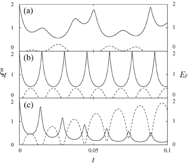
Figure 4: The time evolution of $\xi_{t}$ (solid line, left scale) and the EOF $E_{F}$ (dashed line, right scale) for a symmetric thermal BEC with $N_{a}=N_{b}=400$; $\kappa_{a}=\kappa_{b}=1$; $\Omega_{a}=\Omega_{b}=50$; $\bar{n}_{a}=\bar{n}_{b}=0.5$; and (a) $\kappa=0.50$; (b) $\kappa=1.00$; (c) $\kappa=1.12$.

References

• (1) C.C. Bradley et al., Phys. Rev. Lett. 75, 1687 (1995); K.B. Davis et al., ibid. 75, 3969 (1995); M.H. Anderson et al., Science 269, 198 (1995).
• (2) A.S. Parkins and D.F. Walls, Phys. Rep. 303, 1 (1998).
• (3) A.J. Leggett, Rev. Mod. Phys. 73, 307 (2001) and references therein.
• (4) B.P. Anderson and M.A. Kasevich, Science 282, 1686 (1998); F.S. Cataliotti et al., ibid. 293, 843 (2001).
• (5) A. Sorensen, L.M. Duan, I. Cirac and P. Zoller, Nature (London) 409, 63 (2001).
• (6) L.M. Duan, J.I. Cirac and P. Zoller, Phys. Rev. A 65, 033619 (2002).
• (7) Özgür E. Müstecaplioğlu, M. Zhang and L. You, Phys. Rev. A 66, 033611 (2000).
• (8) D. Bouwmeester et al., Nature (London) 390, 575 (1997).
• (9) D. Boschi et al., Phys. Rev. Lett. 80, 1121 (1998).
• (10) C.J. Myatt et al., Phys. Rev. Lett. 78, 586 (1997).
• (11) D.S. Hall et al., Phys. Rev. Lett. 81, 1539 (1998).
• (12) T.-L. Ho and V.B. Shenoy, Phys. Rev. Lett. 77, 3276 (1996).
• (13) E.V. Goldstein, M.G. Moore, H. Pu and P. Meystre, Phys. Rev. Lett. 85, 5030 (2000).
• (14) C.K. Law, H.T. Ng and P.T. Leung, Phys. Rev. A 63, 055601 (2001).
• (15) G. Modugno et al., Phys. Rev. Lett. 89, 190404 (2002).
• (16) A. Simoni et al., Phys. Rev. Lett. 90, 163202 (2003).
• (17) Sahel Ashhab and Carlos Lobo, Phys. Rev. A 66, 013609 (2002).
• (18) H.T. Ng, C.K. Law and P.T. Leung, Phys. Rev. A 68, 013604 (2003).
• (19) M. Greiner et al., Nature (London) 415, 39 (2002).
• (20) L.M. Duan, G. Giedke, J.I. Cirac and P. Zoller, Phys. Rev. Lett. 84, 2722 (2000).
• (21) R. Simon, Phys. Rev. Lett. 84, 2726 (2000).
• (22) B. Julsgaard, A. Kozhekin and E.S. Polzik, Nature (London) 413, 400 (2001).
• (23) T. Holstein and H. Primakoff, Phys. Rev. 58, 1098 (1949).
• (24) G. Giedke et al., Phys. Rev. Lett. 91, 107901 (2003).
• (25) G.J. Milburn, J. Corney , E.M. Wright and D.F. Walls, Phys. Rev. A 55, 4318 (1997).
• (26) S. Raghavan, A. Smerzi, S. Fantoni and S.R. Shenoy, Phys. Rev. A 59, 620 (1999).
• (27) J. Javanainen and M.Y. Ivanov, Phys. Rev. A 60, 2351 (1999).
• (28) J.J. Sakurai, Modern Quantum Mechanics (Addison-Wesley, Reading, MA, 1994).
• (29) C. Emary and T. Brandes, Phys. Rev. Lett. 90, 044101 (2003); X. Wang and Barry C. Sanders, Phys. Rev. A 68, 033821 (2003).
• (30) B. Esry and C.H. Greene, Phys. Rev. A 59, 1457 (1999).
• (31) W.K. Wootters, Quantum Inf. Comput. 1, 45 (2001).
• (32) V. Josse et al., Phys. Rev. Lett. 92, 123601 (2004).
• (33) M.O. Scully and M.S. Zubairy, Quantum Optics (Cambridge University Press, Cambridge, 1997).
• (34) G. Vidal, J.I. Latorre, E. Rico, and A. Kitaev, Phys. Rev. Lett. 90, 227902 (2003).
• (35) Y. Shin et al., Phys. Rev. Lett. 92, 150401 (2004).
• (36) S.M. Barnett and P.M. Radmore, Methods in Theoretical Quantum Optics (Clarendon Press, Oxford, 1997).
Refer to caption