Complementarity of Entanglement and Interference

A complementarity relation is shown between the visibility of interference and bipartite entanglement in a two qubit interferometric system when the parameters of the quantum operation change for a given input state. The entanglement measure is a decreasing function of the visibility of interference. The implications for quantum computation are briefly discussed.

PACS Nos: 03.65.Vf,03.65.Yz,03.67.Lx,03.67.Mn

1 Introduction

The well-known complementarity or duality of particle and wave is one of the deepest concepts in quantum mechanics. In this work we investigate a similar complementarity between entanglement and interference, which are both important concepts in quantum mechanics [1] and also powerful tools in quantum information processing [2].

More specifically, we quantify the complementarity of entanglement and interference visibility for a bipartite system within an interferometric model. The entanglement measures for bipartite mixed states were introduced and their significance in quantum processing was discussed by Bennett et al. [3]. An extensive discussion of entanglement measures can be found, e.g., in Horodecki [4] and in Vedral and Plenio [5]. We use the interferometric model of Sjöqvist et al. [6], which introduces internal degrees of freedom for the impinging particle. The authors of Ref. [6] were interested in an experimental approach (recently verified by NMR techniques [7]) to the geometric phase for mixed states. In this model the geometric phase can be observed by a shift of the interference pattern so that the visibility of the latter and that of the geometric phase are the same thing.

Here we show that, for any bipartite system of path and internal degrees of freedom, the entanglement measure of the compound output state (the negativity in the two qubits mixed case and the von Neumann entropy of the reduced density operator in the case of pure states with arbitrary dimensions) is a decreasing function of the visibility of the interference in the counting rate of outgoing particles, where the control parameters of the quantum operation change for a given input.

We should stress that in the present literature a number of works appeared dealing with topics close to ours to various extents. Complementarity relations between single and two particle fringe visibilities were found by Jaeger et al. [8], between distinguishability and visibility by Englert and collaborators [9] etc.. For example, in Englert et al. [10] the wave particle duality is discussed by showing the complementarity between the distinguishability of ”which-way” path and the visibility of interference in Young’s double slit experiment. However, the distinguishability seems qualitatively related to the entanglement but not in a quantitative level. Furthermore, e.g. Jacob and Bergou [11] investigated the relation between the concurrence of entanglement and visibility in a bipartite system. For pure states the authors observed the same complementarity as the one described here in Sec. 4 , while for mixed states they found a weaker statement in the form of an inequality (the relationship between indistinguishability and average predictability and coherence for an arbitrary state of two qubits was also recently analyzed in [12]). Ekert et al. [13] presented a quantum network based on the controlled-SWAP gate, and whose interferometric setup is similar to ours, that can extract certain properties of quantum states without recourse to quantum tomography and can be used as a basic building block for direct quantum estimations of both linear and non-linear functionals of any density operator. Recently, Carteret [14] also constructed an interesting quantum circuit corresponding to the interferometric model which measures the trace of powers of the partially transposed density operator, by which we can compute its spectrum and then the concurrence. Hartley and Vedral [15] finally used a similar method to measure and relate the von Neumann entropy and the geometric phase visibility for two and three dimensional Hilbert spaces.

The paper is organized as follows. We first describe the interferometry model for a two qubit state and give a more specific definition for the entanglement and the visibility of interference in Sec. 2. In Sec. 3 we demonstrate the complementarity of entanglement and interference for a mixed state which has an entanglement boundary in the parameter space. In Sec. 4 we consider a pure bipartite system, while Sec. 5 is devoted to the analytical description of the complementarity relation for a pure bipartite system in arbitrary dimensions. Sec. 6 is finally devoted to a brief summary and a discussion of some of the possible implications of our results on quantum computation.

2 An Interferometry Model

We consider the model of Sjöqvist et al. [6], which is essentially a standard Mach-Zehnder interferometer where the Hilbert space consists of the path states for the impinging particle (e.g., a neutron) and of the states for its internal degrees of freedom (e.g., the spin) (see Figs. 1-2). A detector is set at the output to detect particles moving in the horizontal direction. By means of a phase shifter located along one of the horizontal paths, we can see an interference phenomenon in the counting rate of the horizontally outgoing particles as a function of the phase shift. We are then going to study the relation between the visibility of this interference pattern and a measure of the entanglement between path and internal output states.

Figure 1: Sjöqvist’s interferometer model. Particles (spin: 1/2) entering the interferometer along the horizontal direction are globally phase-shifted by $\chi$ and their spin states are transformed by the unitary $U$. Then the particles are reflected by two mirrors and merge through a beam splitter, after which they are detected in the horizontal direction.

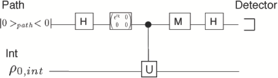
Figure 2: Quantum circuit equivalent to Sjöqvist’s interferometer model.

More in detail, the state of the compound system “path-internal states” will change as

$$\rho_{IN}\rightarrow\rho_{OUT}=V\rho_{IN}V^{\dagger},$$ (1)

where the unitary operator $V$ is given by

$$V\equiv V_{H}V_{M}V_{C}V_{H},$$ (2)

$V_{H}$ represents the unitary transformation corresponding to the beam splitters,

$$V_{H} \equiv H\otimes I,$$

$$H \equiv {1\over\sqrt{2}}\left(\begin{array}[]{clcr}1&~{}~{}1\\ 1&-1\end{array}\right),$$ (5)

while $V_{M}$ is the unitary transformation corresponding to the mirrors,

$$V_{M} \equiv M\otimes I,$$

$$M \equiv \left(\begin{array}[]{clcr}0&1\\ 1&0\end{array}\right).$$ (8)

Note that neither of these operators affect the internal states. The operator $V_{C}$, instead, also acts on the internal space depending on the path travelled by the particle. If the particle passes through the vertical path its internal state undergoes a unitary transformation $U$, while if it passes through the horizontal path it picks up a phase $\chi$. Explicitly,

$$V_{C}\equiv\left(\begin{array}[]{clcr}0&0\\ 0&1\end{array}\right)\otimes U+\left(\begin{array}[]{clcr}e^{i\chi}&0\\ 0&0\end{array}\right)\otimes I.$$ (9)

The input state is chosen as a separable state,

$$\rho_{IN}=|0>_{path}<0|\otimes\rho_{0,int},$$ (10)

describing a particle entering the interferometer device along the horizontal direction ($|0>_{path}$) and with initial internal state $\rho_{0,int}$. Later we take this as represented by a one qubit (spin 1/2) system and consider two typical cases: a pure state $|0>_{int}<0|$ and the general mixed state with the standard Bloch parametrization,

$$\rho_{0,int}\equiv{1\over 2}(I+\vec{b}_{0}\cdot\vec{\sigma}).$$ (11)

The output state is in general entangled and can be expanded as

$$\rho_{OUT} = V\rho_{IN}V^{\dagger}$$ (16)

$$= {1\over 4}\biggl{[}\left(\begin{array}[]{clcr}1&1\\ 1&1\end{array}\right)\otimes U\rho_{0,int}U^{\dagger}+\left(\begin{array}[]{clcr}~{}~{}1&-1\\ -1&~{}~{}1\end{array}\right)\otimes\rho_{0,int}$$

$$+ e^{-i\chi}\left(\begin{array}[]{clcr}1&-1\\ 1&-1\end{array}\right)\otimes U\rho_{0,int}+e^{i\chi}\left(\begin{array}[]{clcr}~{}~{}1&~{}~{}1\\ -1&-1\end{array}\right)\otimes\rho_{0,int}U^{\dagger}\biggr{]}.$$ (21)

The probability to detect the particle in the horizontal direction is given by

$$P_{|0>_{path}} = Tr_{path,int}(|0>_{path}<0|\otimes\rho_{OUT})$$ (22)

$$= {1\over 4}Tr_{int}[U\rho_{0,int}U^{\dagger}+\rho_{0,int}+e^{i\chi}\rho_{0,int}U^{\dagger}+e^{-i\chi}U\rho_{0,int}]$$

$$= {1\over 2}[1+|Tr_{int}(U\rho_{0,int})|\cdot\cos(\chi-arg(Tr_{int}(U\rho_{0,int}))]$$

$$\equiv {1\over 2}[1+\Gamma\cos(\chi-\gamma_{g})].$$

This exhibits an interference pattern in the $\chi$ space with the visibility $\Gamma\equiv|Tr_{int}(U\rho_{0,int})|$ and the shift of the pattern $\gamma_{g}\equiv arg[Tr_{int}(U\rho_{0,int})]$. The latter one is also called the geometric phase for a mixed state $\rho_{0,int}$ (Fig. 3). We would like to stress here that in this interferometric model we start with a separable state and entanglement is achieved through the selective operation $U$ acting on the internal space.

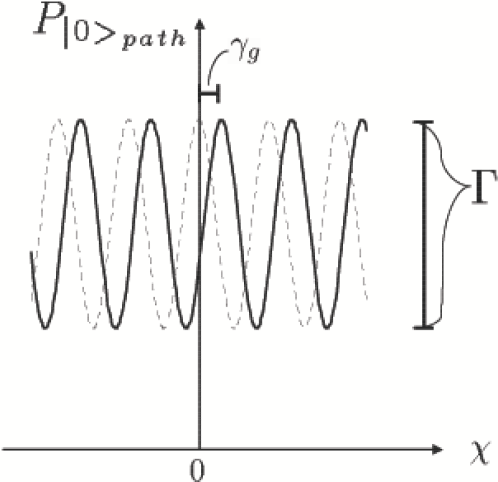
Figure 3: The probability to detect a particle along the horizontal direction at the output of the interferometer shows an interference pattern as a function of the phase shift $\chi$.

3 Entanglement of Mixed State vs. Visibility of Interference

3.1 Parametrization

The density matrix can be explicitly written via the phase $\chi$ and the parametrizations of the initial spin state $\rho_{0,int}$ as given in eq. (11) and that of the unitary transformation $U$ for the spin state as

$$U=\left(\begin{array}[]{clcr}t+iz&ix+y\\ ix-y&t-iz\end{array}\right)\;\;;~{}~{}~{}t^{2}+x^{2}+y^{2}+z^{2}=1.$$ (25)

As a whole we have seven parameters (${\vec{b}}_{0}$, $\chi$ and $t,x,y,z$ with a constraint) in the output state $\rho_{OUT}$. This implies that the density operator output by the interferometer cannot represent a two qubit mixed state in full generality. To realize a completely general density operator one needs nine parameters (apart from the local degrees of $SU(2)\times SU(2)$), which can be achieved by introducing two extra CP operations along the interferometer axes (see Sec. 3.3).

Without loss of generality the input state for the second qubit can be taken as in eq. (11) with $\vec{b}_{0}=b_{0}\vec{e}_{z}$, where the $\vec{e}_{i}$’s are the Bloch sphere orthonormal basis vectors. The output state $\rho_{OUT}$ is given by eq. (21), with the last two terms representing the interference effect, which can be seen more explicitly by the probability to detect the particle in the horizontal direction, according to eq. (22). In our parametrization $Tr_{int}(U\rho_{0,int})=t+ib_{0}z$, so that the visibility $\Gamma$ is

$$\Gamma=\sqrt{t^{2}+b_{0}^{2}\,z^{2}},$$ (26)

while the geometric phase $\gamma_{g}$ is

$$\gamma_{g}=\arctan\left({b_{0}z\over t}\right).$$ (27)

3.2 Negativity

We choose the negativity as a measure of entanglement since it is known to be LOCC monotone [16] and it is easy to compute. The negativity $N(\rho)$ is defined as

$$N(\rho)=2\sum_{\lambda_{i}<0}|\lambda_{i}|,$$ (28)

where the sum is over all negative eigenvalues $\lambda_{i}$’s of $\rho^{PT}$, the partial transposition of the density operator $\rho$. If any of the $\lambda_{i}$’s is negative, the state is entangled according to the criterion of Peres [17], otherwise the state is separable, i.e. the negativity is zero. It is convenient to use Kimura’s method [18] to find the $\lambda_{i}$’s. It is known that there is only one negative eigenvalue $\lambda_{min}$ of $\rho_{OUT}^{PT}$ in the case of two dimensional bipartite mixed states (in general dimensions there may be many). The eigenvalue $\lambda_{min}$ can be either zero or negative, depending on the parameters chosen for the unitary transformation $U$ and on the unknown initial state $\rho_{0,int}$.

Expanding the determinant in the eigenvalue equation we get

$$F(\lambda)\equiv det(\rho_{OUT}^{PT}-\lambda)=\lambda^{4}-a_{1}\lambda^{3}+a_{2}\lambda^{2}-a_{3}\lambda+a_{4},$$ (29)

where the coefficients $a_{i}$’s are given by

$$a_{1} = 1,$$

$$2!a_{2} = 1-Tr_{path,int}({\rho_{OUT}^{PT}}^{2}),$$

$$3!a_{3} = 1-3Tr_{path,int}({\rho_{OUT}^{PT}}^{2})+2Tr_{path,int}({\rho_{OUT}^{PT}}^{3}),$$

$$4!a_{4} = 1-6Tr_{path,int}({\rho_{OUT}^{PT}}^{3})+3[Tr_{path,int}({\rho_{OUT}^{PT}}^{2})]^{2}$$ (30)

$$- 6Tr_{path,int}({\rho_{OUT}^{PT}}^{4}).$$

A straightforward computation gives us

$$a_{1} = 1,$$

$$2!a_{2} = {1-b_{0}^{2}\over 2},$$

$$3!a_{3} = -{3\over 2}b_{0}^{2}(x^{2}+y^{2}),$$

$$4!a_{4} = -{3\over 2}b_{0}^{2}(x^{2}+y^{2})[x^{2}+y^{2}+z^{2}(1-b_{0}^{2})].$$ (31)

It is clear from the fact that $a_{4}>0$ that at least one of the eigenvalues of the partial transposition of the density operator is negative unless $x=y=0$, in which case two of them are zero. Furthermore the roots of ${d^{2}F(\lambda)\over d\lambda^{2}}=0$ are positive because $a_{1}>0$ and $a_{2}>0$. We see that the two points of reflection are positive so that only one of the eigenvalues of the partially transposed density operator is negative as known for a general two qubit case.

Just for illustration let us consider a special case ($t=0$) for the unitary transformation, i.e.

$$U=\left(\begin{array}[]{clcr}iz&ix+y\\ ix-y&-iz\end{array}\right)\;\;;~{}~{}~{}x^{2}+y^{2}+z^{2}=1.$$ (32)

The eigenvalues of $\rho_{OUT}^{PT}$ are then

$$\lambda_{min} = -{b_{0}\sqrt{x^{2}+y^{2}}\over 2},$$

$$\lambda_{2} = {1+b_{0}z\over 2},$$

$$\lambda_{3} = {1-b_{0}z\over 2},$$

$$\lambda_{4} = {b_{0}\sqrt{x^{2}+y^{2}}\over 2},$$ (33)

and therefore, explicitly using eq. (26) for the visibility $\Gamma=b_{0}~{}z$ and the unitarity condition $x^{2}+y^{2}+z^{2}=1$, the negativity reads

$$N(\rho)=\sqrt{b_{0}^{2}-\Gamma^{2}}.$$ (34)

For $t=0$, the geometric phase is $\gamma_{g}={\pi\over 2}$. For a fixed (unknown) input parameter $b_{0}$ the curve (34) is a quadrant of a circle with the radius $b_{0}$. Therefore the entanglement is a decreasing function of the visibility of the geometric phase. The largest entanglement $N=b_{0}$ and the smallest visibility $\Gamma=0$ are obtained for $z=0$. This means a flip of the spin on the vertical path, while the opposite is realized when we do nothing but perform the standard Mach-Zehnder interferometry. In the generic case the visibility is $b_{0}$ times the cosine of the angle by which the spin is tilted by the unitary transformation, while the entanglement is $b_{0}$ times the sine of it. The complementarity comes from the unitarity of the operation $U$. The pure state case that we considered before is reproduced if one puts $b_{0}=1$. For non-zero $t$, we numerically computed the negativity and the visibility and plot them together as a function of $t$ in Fig. 4, with a fixed $b_{0}=0.7$. We can see qualitatively the same phenomenon as the special case $t=0$ for each $t$; the negativity is a monotonically decreasing function of the visibility.

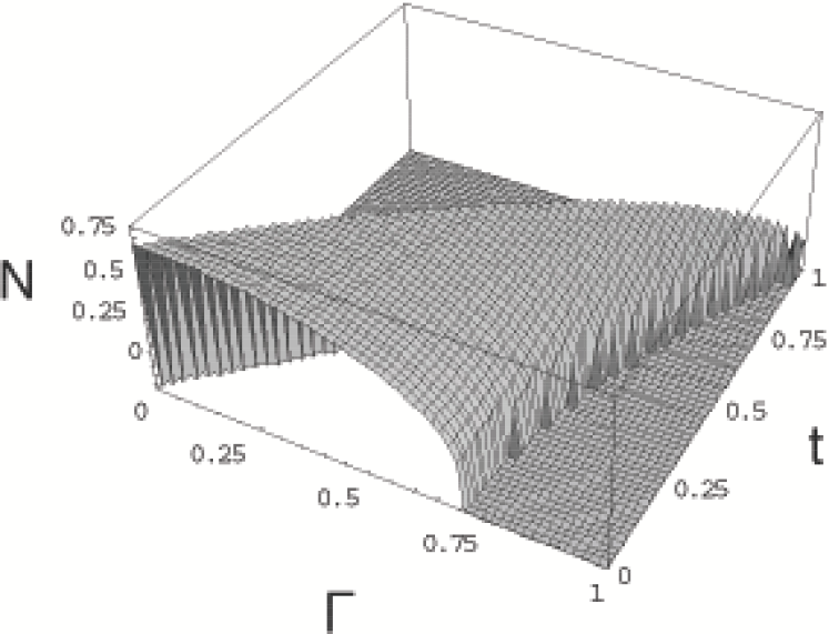
Figure 4: A plot of the negativity N as a function of the visibility $\Gamma$ and the control parameter $t$ of the unitary transformation $U$ for a fixed input parameter $b_{0}~{}(=0.7)$. The flat area represents the physically accessible states when $U$ is parametrized by $t>0$ (see eq. (25)). For a general mixed state $\rho_{0,int}$ and $t\neq 0$, $N$ is a decreasing function of $\Gamma$.

Turning back to the eigenvalue equation for $\rho_{OUT}^{PT}$, this can be more conveniently cast into the form,

$$F(\lambda)=\lambda^{4}-\lambda^{3}+\alpha\lambda^{2}+\beta\lambda-\beta\gamma=0,$$ (35)

where $\alpha\equiv(1-b_{0}^{2})/2$, $\beta\equiv\{b_{0}^{2}-[1-(1-b_{0}^{2})\cos^{2}\gamma_{g}]\Gamma^{2}\}/4$ and $\gamma\equiv(1-\Gamma^{2})/4$. Note that the ranges of the parameters are $0\leq\alpha\leq 1/2$, $0\leq\beta\leq 1/4$ and $0\leq\gamma\leq 1/4$ and also the fact that the visibility dependence appears only in the terms $\beta$ and $\gamma$. Regarding $\lambda$ as the smallest (negative) eigenvalue of $F(\lambda)$, taking the derivative of $F(\lambda)$ with respect to $\Gamma$ and using $N(\rho)=-2\lambda$, we get:

$${\partial F(\lambda)\over\partial\lambda}\cdot{dN(\rho)\over d\Gamma}=\Gamma[\beta+(\gamma+|\lambda|)\delta]>0,$$ (36)

where $\delta\equiv[1-(1-b_{0}^{2})\cos^{2}\gamma_{g}]>0$. Therefore, since $\lambda$ is the smallest root of the quartic form, so that the derivative ${\partial F(\lambda)\over\partial\lambda}$ is negative, we conclude that ${dN(\rho)\over d\Gamma}<0$.

3.3 General Mixed State of Two Qubits via CP Maps

The model of the previous sections can be generalized by further applying on both arms of the interferometer (after the two mirrors) two CP maps (Fig. 5). The first is given by $W_{1}$, which acts as

$$W_{1}:\rho_{1}~{}\rightarrow~{}\rho_{2}\equiv(1-p)\rho_{1}+pA_{1}\rho_{1}A_{1}^{\dagger},$$ (37)

where $\rho_{1}\equiv V_{0}\rho_{IN}V_{0}^{\dagger}$, with $V_{0}\equiv V_{M}V_{C}V$, is the density matrix after the mirrors, the parameter $p\in[0,1]$ and $A\equiv 1\otimes\sigma_{x}$. In other words, $W_{1}$ may represent the chance of a bit-flip noise in the internal degrees of freedom with probability $p$. The second CP map, acting immediately after $W_{1}$, is then given by

$$W_{2}:\rho_{2}~{}\rightarrow~{}\rho_{3}\equiv(1-q)\rho_{2}+qA_{2}\rho_{2}A_{2}^{\dagger},$$ (38)

where now the operator $A_{2}\equiv\sigma_{z}\otimes 1$ represents the chance of a phase noise in the beam (caused, e.g., by an imprecise notion of the location of the mirrors) with probability $q\in[0,1]$. It is important to note that, although these two CP maps of course do not represent the most general situation of possible sources of noise in the system (there might be other kinds of noise, and in different locations in the interferometer), the model we consider is already sufficient to realize a two qubit mixed state with nine parameters ($\vec{b}_{0},\chi,p,q$ and $t,x,y,z$ modulo the unitarity constraint for $U$), i.e. the most arbitrary four dimensional density matrix once the local $SU(2)\times SU(2)$ operations are modded out.

The mixed state finally goes through the last beam splitter, $\rho_{OUT}\equiv V_{H}\rho_{3}V_{H}^{\dagger}$ and one thus obtains the output parametrized as

$$\rho_{OUT}\equiv{1\over 4}[I\otimes I+\vec{a}\cdot\vec{\sigma}\otimes I+I\otimes\vec{b}\cdot\vec{\sigma}+c_{ij}\sigma_{i}\otimes\sigma_{j}],$$ (39)

where

$$\vec{a} \equiv \alpha_{q}[-(t\sin\chi-b_{0}z\cos\chi)\vec{e}_{y}+(t\cos\chi+b_{0}z\sin\chi)\vec{e}_{z}],$$

$$\vec{b} \equiv b_{0}\{(-ty+xz)\vec{e}_{x}+\alpha_{p}[(tx+yz)\vec{e}_{y}+(t^{2}+z^{2})\vec{e}_{z}]\},$$

$$\vec{c}_{x} \equiv b_{0}\{(-ty+xz)\vec{e}_{x}+\alpha_{p}[(tx+yz)\vec{e}_{y}-(x^{2}+y^{2})\vec{e}_{z}]\},$$

$$\vec{c}_{y} \equiv \alpha_{q}\{(x\cos\chi+b_{0}y\sin\chi)\vec{e}_{x}+\alpha_{p}[(y\cos\chi-b_{0}x\sin\chi)\vec{e}_{y}$$

$$+ (z\cos\chi-b_{0}t\sin\chi)\vec{e}_{z}]\}],$$

$$\vec{c}_{z} \equiv \alpha_{q}\{(x\sin\chi-b_{0}y\cos\chi)\vec{e}_{x}+\alpha_{p}[(y\sin\chi+b_{0}x\cos\chi)\vec{e}_{y}$$ (40)

$$+ (z\sin\chi+b_{0}t\cos\chi)\vec{e}_{z}]\}].$$

We have here chosen, without loss of generality, $\vec{b}_{0}=b_{0}\vec{e}_{z}$, and we have redefined for simplicity the parameters $(p,q)$ in terms of $\alpha_{p}\equiv 1-2p$ and $\alpha_{q}\equiv 1-2q$ ($\alpha_{p,q}\in[-1,1]$). Moreover, we have decomposed the matrix $c_{ij}$ appearing in the last term of eq. (39) as the column vector $c\equiv(\vec{c}_{x},\vec{c}_{y},\vec{c}_{z})^{T}$.

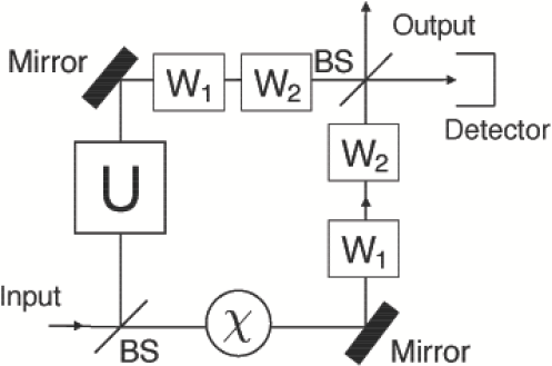
Figure 5: Sjöqvist’s interferometer model with the extra CP maps, $W_{1}$ and $W_{2}$. With probability $p$ the spin state of the particles is bit-flipped ($W_{1}$) and with probability $q$ the beam state gets a phase shift $(W_{2})$.

The probability to detect the particle in the horizontal direction after the last beam splitter is still given by eq. (22), but now the visibility is scaled down by the factor $\alpha_{q}$, i.e.

$$\Gamma=|\alpha_{q}|\sqrt{t^{2}+b_{0}^{2}z^{2}},$$ (41)

and the geometric phase (27) also acquires an extra contribution from $arg(\alpha_{q})$. We can now proceed to evaluate the negativity as our measure of entanglement. As an example, we consider the analytically solvable model where the parameters $t$ and $x$ are chosen to be zero. In this case, the coefficients $a_{i}$’s in the eigenvalue equation (29) for the partial transpose of the output density matrix can be compactly written as

$$a_{2} = {1\over 4}[(1-b_{0}^{2})+2(1+b_{0}^{2})(\mu_{p}+\mu_{q})-8\mu_{p}\mu_{q}],$$

$$a_{3} = {1\over 4}\{-b_{0}^{2}(1-z^{2})+[1+b_{0}^{2}(3-4z^{2})](\mu_{p}+\mu_{q})$$

$$- 4[1+2b_{0}^{2}(1-2z^{2})]\mu_{p}\mu_{q}\},$$

$$a_{4} = {1\over 16}\{-b_{0}^{2}(1-z^{2})(1-b_{0}^{2}z^{2})[1-4(\mu_{p}+\mu_{q})]+(1-b_{0}^{2})^{2}(\mu_{p}^{2}+_{m}u_{q}^{2})$$ (42)

$$+ 2[1-8b_{0}^{2}(1-z^{2})-b_{0}^{4}(1-8z^{2}+8z^{4})]\mu_{p}\mu_{q}$$

$$- 8(1-b_{0}^{2})\mu_{p}\mu_{q}(\mu_{p}+\mu_{q})+16\mu_{p}^{2}\mu_{q}^{2}\},$$

where the effects of the non zero probabilities for the bit-flip and phase noise are explicitly shown through the parameters $\mu_{p}\equiv(1-\alpha_{p}^{2})/4=p(1-p)$ and $\mu_{q}\equiv(1-\alpha_{q}^{2})/4=q(1-q)$, and the dependence on the visibility must be seen through the substitution $z^{2}=\Gamma^{2}/\alpha_{q}^{2}b_{0}^{2}$. It is then immediate to calculate the eigenvalues of the partial transpose $\rho_{OUT}^{PT}$ as

$$\lambda_{1} = {1\over 4}[1-\alpha_{p}\alpha_{q}-\sqrt{b_{0}^{2}(\alpha_{p}+\alpha_{q})^{2}-4\Gamma^{2}\alpha_{p}/\alpha_{q}}],$$

$$\lambda_{2} = {1\over 4}[1+\alpha_{p}\alpha_{q}-\sqrt{b_{0}^{2}(\alpha_{p}-\alpha_{q})^{2}+4\Gamma^{2}\alpha_{p}/\alpha_{q}}],$$

$$\lambda_{3} = {1\over 4}[1-\alpha_{p}\alpha_{q}+\sqrt{b_{0}^{2}(\alpha_{p}+\alpha_{q})^{2}-4\Gamma^{2}\alpha_{p}/\alpha_{q}}],$$

$$\lambda_{4} = {1\over 4}[1+\alpha_{p}\alpha_{q}+\sqrt{b_{0}^{2}(\alpha_{p}-\alpha_{q})^{2}+4\Gamma^{2}\alpha_{p}/\alpha_{q}}].$$ (43)

After some algebra (which we omit here for the sake of simplicity), one can show that for a certain region of the parameters $(\alpha_{p},\alpha_{q})$ (i.e., $(p,q)$) such that $\alpha_{p}\alpha_{q}>0$, the minimal and negative eigenvalue is given by $\lambda_{1}$, while for another region for which $\alpha_{p}\alpha_{q}<0$ the minimal and negative eigenvalue is $\lambda_{2}$. As an example, in the case in which there is only the chance of bit-flip noise (i.e., $q=0$), we get that $\lambda_{1}<0$ for $0<p<p_{-}<1/2$ and $\lambda_{2}<0$ for $1/2<p<p_{+}<1$, where $p_{-}\equiv\sqrt{b_{0}^{2}-\Gamma^{2}}(\sqrt{1-\Gamma^{2}}-\sqrt{b_{0}^{2}-\Gamma^{2}})/(1-b_{0}^{2})$ and $p_{+}\equiv\sqrt{1-\Gamma^{2}}(\sqrt{1-\Gamma^{2}}-\sqrt{b_{0}^{2}-\Gamma^{2}})/(1-b_{0}^{2})$.

For general $(p,q)$, unifying the cases with different signs for the product $\alpha_{p}\alpha_{q}$, we then obtain the negativity as

$$N={1\over 2}[-1+|\alpha_{p}||\alpha_{q}|+\sqrt{b_{0}^{2}(|\alpha_{p}|+|\alpha_{q}|)^{2}-4\Gamma^{2}|\alpha_{p}|/|\alpha_{q}|}].$$ (44)

As a consequence, similarly to the case studied in the previous paragraphs, we obtain the following two results. First, in the regions where the negativity is non zero, i.e. where the output mixed state is entangled, there is a simple geometric relationship between the visibility and the negativity, which can be seen by rewriting eq. (44) as

$${N^{\prime 2}\over a^{2}}+{\Gamma^{2}\over b^{2}}=1,$$ (45)

which clearly represents an ellipse centered at $N^{\prime}\equiv N+(1-|\alpha_{p}||\alpha_{q}|)/2=\Gamma=0$ with semiaxis $a\equiv b_{0}(|\alpha_{p}|+|\alpha_{q}|)/2$ and $b\equiv\sqrt{|\alpha_{q}|/|\alpha_{p}|}a$. In other words, the negativity is maximum, $N=[b_{0}(|\alpha_{p}|+|\alpha_{q}|)-(1-|\alpha_{p}||\alpha_{q}|)]/2$ when the the visibility is zero, and vice versa when the negativity is minimum, i.e. zero, the visibility is maximum, ranging as $\Gamma\in[\{b_{0}^{2}(|\alpha_{p}|+|\alpha_{q}|)^{2}-(1-|\alpha_{p}||\alpha_{q}|)^{2}|\alpha_{q}|/|\alpha_{p}|\}^{1/2}/2,|\alpha_{q}|b_{0}]$. In Fig. 6 we numerically plotted the values of the negativity $N$ as a function of the visibility $\Gamma$ and the control parameter $t$ for the case of a bit-flip noise model with fixed $x=0.4$ and the set of probabilities $p=0.4$ and $p=0.5$. The second, related, result is again the complementarity between the visibility and the negativity, which is mathematically expressed as $dN/d\Gamma=-|\alpha_{p}|/[4|\alpha_{q}|\Gamma\sqrt{b_{0}^{2}(|\alpha_{p}|+|\alpha_{q}|)^{2}-4\Gamma^{2}|\alpha_{p}|/|\alpha_{q}|}<0$. As the careful reader will have already noticed, our extended interferometer model with CP maps has also another property, i.e. the mixed output states can be either entangled or separable, depending on the values chosen for the control parameters $p,q$, $t,x,y,z$ and $\chi$. This had to be expected since our model, equipped with the full set of nine parameters, is able to represent the most general state of a two qubits mixed system. In particular, the boundary between the region with entangled states and that with separable ones is fixed by the condition $a_{4}=0$. In the simple model in which there is only a bit flip noise, i.e. $q=0$, it is immediate to check that the entangled states are given for $0<p<p_{-}$ or $p_{+}<p<1$ (obviously, these are the same parameter ranges for which one of the eigenvalues of $\rho_{OUT}^{PT}$ is negative, i.e. for which the negativity is non zero), while the separable states are for $p_{-}<p<p_{+}$. In other words, at least within our model, the more random the noise in the qubit representing the internal degree of freedom, the less entangled the global mixed state appears to be.

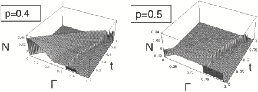
Figure 6: A plot of the negativity N as a function of the visibility $\Gamma$ and the control parameter $t$ of the unitary transformation $U$ for the output of the Sjöqvist’s interferometer model with the extra CP map representing a bit-flip noise, $W_{1}$ $(q=0)$. The input parameter $b_{0}=0.7$, the unitary transformation control parameter $x=0.4$ and the CP map parameter $p=0.4(0.5)$ are fixed. The lowest flat areas in both graphs represent the regions of the physically inaccessible states for the unitary transformation control parameter $t>0$ (see eq. (25)). Note the existence of a boundary between regions with separable states $(N=0)$ and entangled states $(N>0)$ when $p=0.4$. In this case $N(>0)$ is a decreasing function of $\Gamma$. When $p=0.5$ there are only separable states.

4 Entanglement of Pure State vs. Visibility of Interference

The entanglement measure of a bipartite pure quantum system is well established and quantified as the von Neumann entropy of the reduced density operator given by tracing over the internal states,

$$\rho_{red}=Tr_{int}(\rho_{OUT})={1\over 2}[I+\Gamma(\sin(\chi-\phi)\sigma_{y}+\cos(\chi-\phi)\sigma_{z})].$$ (46)

This state is depicted in the Bloch ball (Fig. 7) as a vector with length given by the visibility $\Gamma$ and tilted by the angle $\chi-\phi$ from the z-axis. The entanglement measure is the von Neumann entropy,

$$E=S(\rho_{red})=-\lambda_{+}\log\lambda_{+}-\lambda_{-}\log\lambda_{-},$$ (47)

where $\lambda_{\pm}$ are the eigenvalues of the reduced density matrix $\rho_{red}$, expressed in terms of the visibility $\Gamma$ as

$$\lambda_{\pm}={1\pm\Gamma\over 2}.$$ (48)

This implies that the more visible the interference, the less entangled the state (Fig. 8).

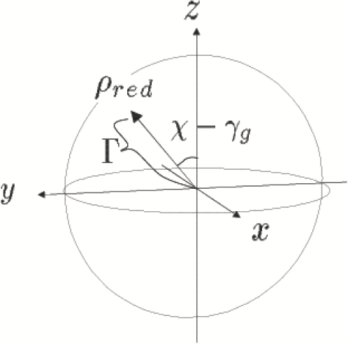
Figure 7: The reduced density matrix as a vector in the Bloch ball. The length of the vector is the visibility and its polar angle is $\chi-\gamma_{g}$, with $\gamma_{g}$ the geometric phase.

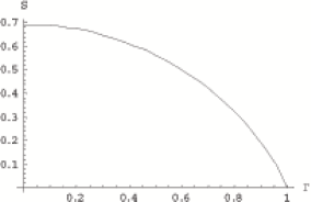
Figure 8: The von Neumann entropy $S$ of the reduced density matrix (the entanglement measure for the pure state) is a decreasing function of the visibility $\Gamma$ of the interference.

5 Complementarity for Pure Bipartite States in Arbitrary Dimensions

While in the previous section entanglement was achieved by the action of the interferometer, in this section, for analytical purposes, we want to start with an already entangled state in Schmidt form and further perform a unitary transformation on the path states. Of course, in the case of two qubit pure states the two approaches are mathematically equivalent. In fact, to see this, we can simply choose the initial internal state to be pure, i.e. $\rho_{0,int}\equiv|\psi_{0}>_{int}<\psi_{0}|$, where $|\psi_{0}>_{int}\equiv a|0>_{int}+b|1>_{int}$, with $a$ and $b$ real parameters satisfying $a^{2}+b^{2}=1$ (or, equivalently, $\vec{b_{0}}=(0,2ab,a^{2}-b^{2})$, with $|\vec{b_{0}}|=1$) and take $U=\sigma_{z}$ to find that the output state in Eq. (21) reads as $\rho_{OUT}=|\psi_{OUT}><\psi_{OUT}|$ with

$$|\psi_{OUT}> = a(\cos{\chi\over 2}|0>_{path}-i\sin{\chi\over 2}|1>_{path})|0>_{int}$$ (49)

$$+ b(\cos{\chi\over 2}|1>_{path}+i\sin{\chi\over 2}|0>_{path})|1>_{int}.$$

Furthermore, this can be derived from the initial entangled state in Schmidt form

$$|\psi_{IN}>=a|0>_{path}|0>_{int}+b|1>_{path}|1>_{int}$$ (50)

by operating on the path space with the unitary transformation $|0>_{path}\rightarrow\cos{\chi\over 2}|0>_{path}-i\sin{\chi\over 2}|1>_{path}$, $|1>_{path}\rightarrow i\sin{\chi\over 2}|0>_{path}+\cos{\chi\over 2}|1>_{path}$

Now we can proceed in the analysis by observing the first qubit without caring about the second one. The probability to get the state $|0>_{path}$ is (cf. Eq. (22))

$$P_{|0>_{path}}={1\over 2}[1+(a^{2}-b^{2})\cos\chi],$$ (51)

which is a typical interference pattern if we regard the angle $\chi$ as a control parameter. The visibility of the interference is

$$\Gamma\equiv|a^{2}-b^{2}|,$$ (52)

which vanishes when the initial state $|\psi_{IN}>$ is maximally entangled, i.e. $a^{2}=b^{2}=1/2$, while it becomes maximum when $|\psi_{IN}>$ is separable, i.e. $a=0$ or $b=0$. On the other hand, by choosing the negativity $N=2|ab|$ as our entanglement measure, we clearly see the complementarity as

$$N^{2}+\Gamma^{2}=1.$$ (53)

We note that this constraint between the entanglement and the interference comes from the unitarity $a^{2}+b^{2}=1$. Alternatively, taking the entanglement measure as the von Neumann entropy we get

$$E\equiv S(\rho_{red})=-a^{2}\log a^{2}-b^{2}\log b^{2},$$ (54)

where the reduced density operator $\rho_{red}\equiv Tr_{int}|\psi_{OUT}><\psi_{OUT}|=Tr_{int}|\psi_{IN}><\psi_{IN}|=a^{2}|0>_{path}<0|+b^{2}|1>_{path}<1|$. The entanglement takes the maximum value $E=1$ when $a^{2}=b^{2}=1/2$ and the minimum value $E=0$ for $a=0$ or $b=0$. Again, we observe that the more the state is entangled, the less is the visibility of the interference and vice versa.

One can also ask to what extent the complementarity holds for general dimensions. Consider a bipartite system initially in the state $|\Psi_{IN}>\in{\cal H}_{path}\otimes{\cal H}_{int}$ of dimensions $n\times n$ given in a Schmidt decomposition form:

$$|\Psi_{IN}>=\sum_{m=1}^{n}\sqrt{c_{m}}|m>_{path}|m>_{int},$$ (55)

with $c_{m}\geq 0,~{}\sum_{m=1}^{n}c_{m}=1$ and $|m>_{path}\in{\cal H}_{path},|m>_{int}\in{\cal H}_{int}$. Suppose then we perform a local unitary transformation $U_{path}$ to the state $|m>_{path}\in{\cal H}_{path}$,

$$|\Psi_{IN}>\rightarrow|\Psi_{OUT}>=\sum_{m=1}^{n}\sqrt{c_{m}}U_{path}|m>_{path}|m>_{int},$$ (56)

and observe the state belonging to ${\cal H}_{path}$. The probability to obtain $|0>_{path}$ is

$$P_{|0>_{path}}(U_{int})=\sum_{m=1}^{n}c_{m}|_{path}<0|U_{path}|m>_{path}|^{2}.$$ (57)

The dependence of $P_{|0>_{path}}(U_{path})$ as a function of the control parameters identifying $U_{path}$ again exhibits an interference pattern. To identify the visibility of the interference pattern $\Gamma$ we subtract the average of $P_{|0>_{path}}(U_{path})$ over $U_{path}$, i.e. $\int P_{|0>_{path}}(U_{path})dU_{path}/\int dU_{path}=1/n$, from the maximum of the intensity,

$${\Gamma\over 2}\equiv Max_{U_{path}}P_{|0>_{path}}(U_{path})-{1\over n}=c_{max}-{1\over n},$$ (58)

where, without loss of generality, we have chosen $c_{max}$ to be the greatest Schmidt coefficient (note that for the simple entangled state given by Eq. (1), $c_{max}=a^{2}$ if $a^{2}\geq b^{2}$ and $n=2$, and then $\Gamma=2(a^{2}-1/2)=a^{2}-b^{2}$, as it should be).

This expression has to be compared with the entanglement entropy

$$E=-\sum_{m=1}^{n}c_{m}\log c_{m}.$$ (59)

With the normalization condition for the Schmidt coefficients $\sum_{m=1}^{n}c_{m}=1$ in mind we see that, fixing all the $c$’s except $c_{max}$ and $c_{k}$,

$${\partial E\over\partial c_{max}}=-\log{c_{max}\over c_{k}}\leq 0.$$ (60)

We can thus conclude that the entanglement $E$ is a decreasing function of $\Gamma$ also for the case of bipartite systems in pure states of arbitrary dimensions. A keen reader may realize that an analogous phenomenon is ubiquitous in quantum information processing: entanglement tends to hinder efficient interference.

6 Summary and Discussion

We have shown the existence of a complementarity relation between the visibility of interference and bipartite entanglement for a generic two qubit mixed state in an interferometric system and for bipartite pure states in arbitrary dimensions. Explicitly, for bipartite pure states in arbitrary dimensions, the von Neumann entropy, which is the unique measure for entanglement, is a decreasing function of the visibility of interference. In the case of two qubit mixed states the same complementarity relation holds, with the negativity taking the role of the entanglement measure. However, there is no unique measure of entanglement for mixed states [4], so that it remains to be seen whether our result is still valid for other measures. The phenomenon described in this paper can be seen as the analogue of the complementarity of the Stern-Gerlach experiment and Young’s double slit experiment. The former is normally performed in the setting in which the spin and the path are maximally entangled so that there is no interference pattern, while the polarizations are not entangled to the paths in Young’s interference experiment. Another example of the complementarity is the dephasing phenomenon, because the interferometric system becomes entangled with the environment. The complementarity may also open up the possibility to quantitatively measure the entanglement by looking at the visibility of the interference (see, e.g., Ref. [14]).

Interestingly enough the issue of entanglement and interference in basic science has a direct implication in quantum computation, in the sense that the complementarity might be a useful tool to analyze its efficiency. Quantum computation is usually assumed to start with a standard separable state and then to make a series of unitary transformations to create a particular entangled state, i.e.

$$\sum_{k}|k>|f(k)>,$$ (61)

so as to obtain the many candidates for the solutions to a given problem characterized by the function $f(k)$ in a quantum parallel way.

In the case of Shor’s algorithm, $f(k)$ is a periodic function of $k$. Suppose we observe the second state to obtain $f(k*)$. The whole state collapses to a superposition

$$\sum_{k,f(k)=f(k*)}|k>|f(k*)>.$$ (62)

The period can be read off by doing a local Fourier transformation on the first state and then looking at the interference pattern. We can clearly see that the observation of the second state cuts the entanglement to make the interference possible.

In general, to solve meaningfully a complex problem one might need sufficient entanglement while also requiring sufficient interference to get the result efficiently. It would be intriguing if a kind of complementarity similar to that analyzed in our work were playing a prominent and decisive role in this process.

We have to caution the reader that the entanglement discussed in the present work is limited to that of bipartite systems. Jozsa and Linden [21] discussed the role of entanglement which spreads over an entire set of qubits in a quantum computation. If we can quantify entanglement for macroscopic systems, it would be very interesting to compare that with the visibility of interference, e.g. in Shor’s algorithm.

References

- [1] A. Peres, Quantum Theory: Concepts and Methods, (Kluwer Academic Publishers, Dordrecht, 1995).
- [2] M.A. Nielsen and I.L. Chuang, Quantum Computation and Quantum Information, (Cambridge University Press, Cambridge, 2000).
- [3] C.H. Bennett, G. Brassard, S. Popescu, B. Schumacher, J.A. Smolin and W.K. Wootters , Phys. Rev. Lett. 76 , 722 (1996).
- [4] M. Horodecki, Quantum Inf. and Comp. 1, 3 (2001).
- [5] V. Vedral and M.B. Plenio, Phys. Rev. A 57, 1619 (1998).
- [6] E. Sjöqvist, A.K. Pati, A. Ekert, J.S. Anandan, M. Ericsson, D.K.L. Oi and V. Vedral, Phys. Rev. Lett. 85 , 2845 (2000).
- [7] J. Du, P. Zou, M. Shi, L.C. Kwek, J.W. Pan, C.H. Oh, A. Ekert, D.K.L. Oi and M. Ericsson, Phys. Rev. Lett. 91, 100403 (2003).
- [8] G. Jaeger, M.A. Horne and A. Shimony, Phys. Rev. A 48, 1023 (1993); G. Jaeger, A. Shimony and L. Vaidman, Phys. Rev. A 51, 54 (1995).
- [9] B.G. Englert, Phys. Rev. Lett. 77, 2154 (1996).
- [10] B.G. Englert and J.A. Bergou, Opt. Commun. 179, 337 (2000).
- [11] M. Jakob and J.A. Bergou, quant-ph/0302075.
- [12] T.E. Tessier, quant-ph/0403022.
- [13] A. K. Ekert, C. Moura Alves, D. K. L. Oi, M. Horodecki, P. Horodecki and L. C. Kwek Phys. Rev. Lett. 88, 217901 (2002).
- [14] H.A. Carteret, quant-ph/0309216.
- [15] J. Hartley and V. Vedral, quant-ph/0309088.
- [16] G. Vidal and R.F. Werner, Phys. Rev. A 65, 032314 (2002).
- [17] A. Peres, Phys. Rev. Lett. 77 , 1413 (1996).
- [18] G. Kimura, Phys. Letters A314, 339 (2003).
- [19] S. Durr, T. Nonn and G. Rempe, Phys. Rev. Lett. 81, 5705 (1998).
- [20] M.J. Donald, M. Horodecki and O. Rudolph, J. Math. Phys. 43, 4252 (2002).
- [21] R. Jozsa and N. Linden, quant-ph/0201143.