New intensity and visibility aspects of a double loop neutron interferometer

Abstract

Various phase shifters and absorbers can be put into the arms of a double loop neutron interferometer. The mean intensity levels of the forward and diffracted beams behind an empty four plate interferometer of this type have been calculated. It is shown that the intensities in the forward and diffracted direction can be made equal using certain absorbers. In this case the interferometer can be regarded as a $50/50$ beam splitter. Furthermore the visibilities of single and double loop interferometers are compared to each other by varying the transmission in the first loop using different absorbers. It can be shown that the visibility becomes exactly $1$ using a phase shifter in the second loop. In this case the phase shifter in the second loop must be strongly correlated to the transmission coefficient of the absorber in the first loop. Using such a device homodyne-like measurements of very weak signals should become possible.

1 Introduction

Neutron interferometry is already a well known method for investigation of coherent matter wave properties. Many features of neutron waves have been analyzed such as coherence and post - selection effects, the spinor symmetry, the magnetic Josephson effect, the multi - photon exchange interaction, spin superposition problems, the Aharonov - Bohm effect, topological phases, gravitationally induced quantum interference, the Sagnac effect, the neutron Fizeau effect et cetera [1].

In this paper we concentrate on coherence effects in a double loop interferometer [2],[3]. Fig.(1) describes an extension of a standard three - plate neutron interferometer where a second loop is added by using a second mirror crystal M2 and where various phase shifters $\Delta$ and absorbers $\alpha$ can be inserted in each loop. Both loops are coupled via beam $(d)$ and therefore most attention will be given to the action of an absorbing phase shift in this beam. We focus on two phase shifters $\Delta_{d}$ and $\Delta_{f}$ and two absorbers $\alpha_{d}$ and $\alpha_{f}$ in beam $(d)$ and $(f)$ respectively because phase shifters or absorbers in beam $(b)$ are of no additional significance.

The paper is organized as follows. In section $2$ intensity aspects of the double loop interferometer are considered. In spite of the non symmetric diffraction properties of neutrons in single crystals it can be shown that a $50/50$ intensity split-up can be reached using an absorber in loop $B$. One of the main findings of the analysis of the double loop interferometer in section $3$ is that the visibility of $K_{0}$ in the forward beam can be made very high (ideally $1$), even for very weak input signals. In section $4$ the results are discussed in detail taking into account real experimental situations.

The main aim is to find an interaction where small signals transmitted through phase shifter $\Delta_{d}$ can be detected with high precision. In this respect it is a search for homodyne-like detection of weak neutron signals by the constrain that a symmetric beam splitter does not exist in case of diffraction from a crystal. The new system consists of a coupled double loop perfect crystal system and provides a symmetric beam splitting or can serve as a basic of homodyne neutron detection in a similar sense as known for photon beams [4].

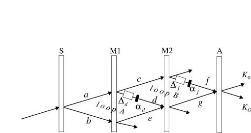
Figure 1: Double loop neutron interferometer: there are three beam pathes: $(acf)$, $(adg)$ and $(beg)$. $\Delta_{d}$ and $\Delta_{f}$ are two phase shifters, $\alpha_{d}$ and $\alpha_{f}$ are two absorbers, $K_{0}$ and $K_{G}$ denote the intensity in the forward and diffracted direction respectively. S is the beam splitter crystal, M1 and M2 are two mirror crystals and A is the analyzer crystal. All four crystal plates have the same thickness $D$ and have equal distance from each other. The first loop (loop $A$) is formed by the beams $(adeb)$, the second loop (loop $B$) by the beams $(cfgd)$. Beam $(g)$ is a superposition of beam $(ad)$ and beam $(be)$.

2 Intensity aspects

From the dynamical theory of diffraction the wave function behind the analyzer crystal in the forward direction (index $0$) which is a superposition of three waves due to the three pathways (s. Fig.(1)) reads as ([1],[5])

$$\psi_{0}^{(acf)+(adg)+(beg)}=\psi_{e}e^{i\gamma}v_{0}^{2}v_{G}v_{0}^{\prime}[e^{ik\Delta_{f}-\alpha_{f}}+e^{ik\Delta_{d}-\alpha_{d}}+1]\,\,\,.$$ (1)

In this expression $\psi_{e}=u_{0}e^{i\bf{kr}}$ is the incoming plane wave function with amplitude $u_{0}$, wave vector $\bf{k}$ and position vector $\bf{r}$ impinging on the beam splitter S. $e^{i\gamma}$ is a phase factor which is of no relevance in the following. The crystal functions $v_{0}$, $v_{G}$ and $v_{0}^{\prime}$ are given as [5]

$$v_{0}=e^{iPD}[cos(\bar{A}\sqrt{1+y^{2}})+iy\frac{sin(\bar{A}\sqrt{1+y^{2}})}{\sqrt{1+y^{2}}}]\,\,\,.$$ (2)

$$v_{G}=-ie^{iPD}\frac{sin(\bar{A}\sqrt{1+y^{2}})}{\sqrt{1+y^{2}}}\,\,\,,\,\,\,v_{0}^{\prime}=v_{G}(-y)\,\,\,.$$ (3)

The index $G$ means the diffracted direction. $P=-{\pi}(1+y)/\Delta_{0}$ and $\bar{A}={\pi}D/\Delta_{0}$ where $\Delta_{0}$ is the Pendelloesung length which is $\Delta_{0}={\lambda}\,cos(\gamma)/|V({\bf{G}})/E|$. $\lambda=2\pi/k\,$ is the wave length and $\gamma$ is the angle between the beam direction and the vector perpendicular to the crystal surface. $|V({\bf{G}})/E|{\approx}10^{-6}$ is the ratio between the crystal potential $V({\bf{G}})$ and the energy $E$ of the particles where $\bf{G}$ is the reciprocal lattice vector corresponding to the reflection plane under consideration. $\Delta_{0}=0.00641\,cm$ for the $(2,2,0)-$ reflection of $2\AA$ neutrons in a silicon single crystal. The quantity $\bar{A}$ is proportional to the crystal thickness $D$. The quantity $y$ depends on the deviation from the Bragg angle. For symmetric diffraction $y$ is defined as $y=k{\,}sin(2\theta_{B}){\,}(\theta_{B}-\theta)/|V({\bf{G}})/E|$. $y=0$ gives the exact direction of the Bragg angle $\theta=\theta_{B}$. The crystal function $v_{0}$ describes the diffraction property of the wave function through a single crystal of thickness $D$. $v_{G}$ characterizes the case of diffraction due to the dynamical theory. The three terms in Eq.(1) form a superposition of three wave functions which belong to the three pathways $(acf)$, $(adg)$ and $(beg)$. They have different phase shifts and absorptions. The crystal functions defined above are equal for each of the three wave functions, because each beam is transmitted (function $v_{0}^{2}$) and diffracted (functions $v_{G}$ and $v_{G}(-y)$) twice respectively.

The wave function in the diffracted direction behind the analyzer crystal reads

$$\psi_{G}^{(acf)+(adg)+(beg)}=\psi_{e^{\prime}}e^{i\delta}v_{0}v_{G}[v_{0}v_{G}^{\prime}e^{ik\Delta_{f}-\alpha_{f}}+v_{G}v_{0}^{\prime}(e^{ik\Delta_{d}-\alpha_{d}}+1)]\,\,\,.$$ (4)

Here, $\psi_{e^{\prime}}=u_{0}e^{i{\bf{k}}_{G}{\bf{r}}}$ is a plane wave function with wave vector ${\bf{k}}_{G}$ pointing to the diffracted direction. $e^{i\delta}$ is a phase factor. The crystal function $v_{G}^{\prime}$ is equal to $v_{0}(-y)$. From Eq.(4) it can be recognized that the three wave functions which are superimposed in the forward direction (0) have the same but those in the diffracted direction $G$ do not have the same number of reflections and transmissions. Therefore an unsymmetrical intensity behavior can be expected in the diffracted direction, as shown below.

In order to compute the intensities $K_{0}$ and $K_{G}$ behind the analyzer crystal the squared moduli of the wave functions, i.e. $|\psi_{0}^{(acf)+(adg)+(beg)}|^{2}$ and $|\psi_{G}^{(acf)+(adg)+(beg)}|^{2}$, have to be taken into account. Because of the thickness of about $0.5$ cm of the crystal plates in Fig.(1) the quantity $\bar{A}={\pi}D/\Delta_{0}>>1$ cause very rapid oscillations of the terms $sin^{2n}(x)$ which appear in these expressions. Therefore the mean values of these trigonometric functions can be used. One gets: $\overline{sin^{2}(x)}=1/2$, $\overline{sin^{4}(x)}=3/8$, $\overline{sin^{6}(x)}=5/16$ and $\overline{sin^{8}(x)}=35/128$ [2]. Moreover integration over the variable $y$ must be performed because of the beam divergence which has to be taken into account. Finally a normalized Gaussian spectral distribution

$$g(k)=\frac{1}{\sqrt{2\pi}(\delta{k})}exp[\frac{(k-k_{0})^{2}}{2(\delta{k})^{2}}]$$ (5)

of incoming wave numbers $k$ is assumed. Here $k_{0}$ is the mean value and $(\delta{k})^{2}$ is the mean square deviation of wave numbers. The intensities can now be calculated (setting $u_{0}=1$) as follows (the limits of integration are always $-\infty$ and $+\infty$):

$$K_{0}=\int{g(k)}[\int{\overline{|\psi_{0}^{(acf)+(adg)+(beg)}|^{2}}}dy]dk=\frac{79\pi}{2048}\{1+e^{-2\alpha_{d}}+e^{-2\alpha_{f}}+$$

$$+2e^{-\alpha_{d}}e^{-(\delta{k})^{2}(\Delta_{d})^{2}/2}cos(\Delta_{d}k_{0})+2e^{-\alpha_{f}}e^{-(\delta{k})^{2}(\Delta_{f})^{2}/2}cos(\Delta_{f}k_{0})+$$

$$+2e^{-(\alpha_{d}+\alpha_{f})}e^{-(\delta{k})^{2}(\Delta_{d}-\Delta_{f})^{2}/2}cos[(\Delta_{d}-\Delta_{f})k_{0}]\}\,\,\,,$$ (6)

$$K_{G}=\int{g(k)}[\int{\overline{|\psi_{G}^{(acf)+(adg)+(beg)}|^{2}}}dy]dk=\frac{\pi}{2048}\{65(1+e^{-2\alpha_{d}})+$$

$$+417e^{-2\alpha_{f}}+130e^{-\alpha_{d}}e^{-(\delta{k})^{2}(\Delta_{d})^{2}/2}cos(\Delta_{d}k_{0})-$$

$$-158e^{-\alpha_{f}}e^{-(\delta{k})^{2}(\Delta_{f})^{2}/2}cos(\Delta_{f}k_{0})-$$

$$-158e^{-(\alpha_{d}+\alpha_{f})}e^{-(\delta{k})^{2}(\Delta_{d}-\Delta_{f})^{2}/2}cos[(\Delta_{d}-\Delta_{f})k_{0}]\}\,\,\,.$$ (7)

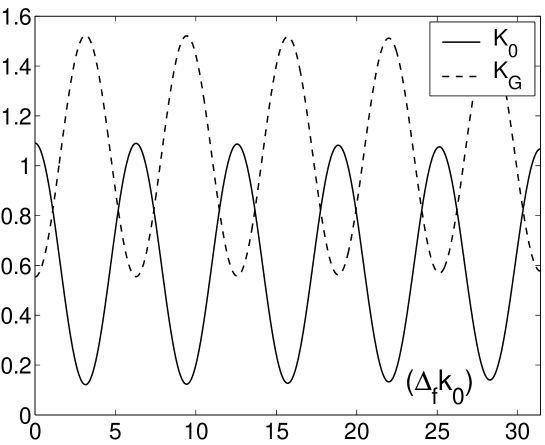
Figure 2: Intensities $K_{0}$ and $K_{G}$ of Eqs.(6) and (7) behind the double loop interferometer (s. Fig.(1)) for $\alpha_{d}=\alpha_{f}=0$, $\Delta_{d}=0$ and $({\delta}k)/k_{0}=1/100$. The level of oscillations of $K_{0}$ is below that of $K_{G}$.

Fig.(2) plots $K_{0}$ and $K_{G}$ for $\Delta_{d}=0$ and $\alpha_{d}=\alpha_{f}=0$ as a function of $\Delta_{f}$. If $\Delta_{f}=0$, $K_{0}=711{\pi}/2048$ and $K_{G}=361{\pi}/2048$. These results can be found elsewhere [2]. One can recognize that the mean intensities of the two beams are - in general - different (just like in single loop interferometry). The question arises if these intensity levels can be made equal by using special parameter values. The answer is yes. If one takes the mean values of $K_{0}$ and $K_{G}$ to be equal, i.e. $\overline{[K_{0}-K_{G}]}_{\Delta_{f}}=0$, one gets a condition for $\alpha_{f}$:

$$\alpha_{f}=-\frac{1}{2}ln{\{}\frac{7}{169}[\,1+e^{-2\alpha_{d}}+2\,e^{-\alpha_{d}}e^{-({\delta}k)^{2}({\Delta}_{d})^{2}}cos(\Delta_{d}k_{0})]{\}}{\geq}0\,\,\,\,.$$ (8)

Any absorption $\alpha$ has to be ${\geq}0$, because the transmission $T=e^{-2\alpha}$ of a beam obeys the relation $0{\leq}T{\leq}1$. In case of $\alpha_{d}=0$ and $\Delta_{d}=0$, the absorption $\alpha_{f}$ becomes $-(1/2)ln(28/169)=0.8988$. Fig.(3) demonstrates this example. In this case the double loop interferometer may be regarded as a $50/50$ beam splitter by using an absorption element in a suitable arm of the device. This is not possible using a single loop interferometer.

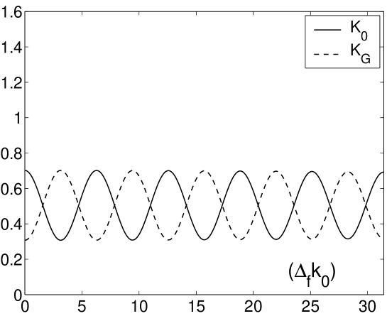
Figure 3: Calculated intensity oscillations of $K_{0}$ and $K_{G}$ of Eqs.(6) and (7) considering the following parameters: $\alpha_{d}=0$, $\alpha_{f}=-(1/2)ln(28/169)=0.8988$, $\Delta_{d}=0$ and $({\delta}k)/k_{0}=1/100$. The intensity levels are equal due to $\alpha_{f}$.

3 Visibilities of single and double loop interferometers

The visibility is defined as

$$V=\frac{I_{max}-I_{min}}{I_{max}+I_{min}}\,\,\,\,\,.$$ (9)

We distinguish two kinds of absorption processes: stochastic (sto) and deterministic (det) absorption [6]. In an interferometer stochastic absorption is realized by inserting an absorbing material in one arm of a beam (s. Fig.(1)). Deterministic absorption can be achieved by a chopper which blocks the beam path periodically or by partial reduction of the beam cross section. In the following we investigate the visibility in a single and double loop interferometer at low interference order (coherence function is approximately $1$).

a) Single loop interferometer (index $1$): If one phase shifter $\Delta_{d}$ and one absorber $\alpha_{d}$ is put in beam path $(d)$, the intensity $I_{0}$ in the forward direction can be written as

$$I_{0}\,{\propto}\,|\,1+e^{ik_{0}\Delta_{d}-\alpha_{d}}|^{2}=1+T_{d}+2\sqrt{T_{d}}{\,}cos(\Delta_{d}k_{0})\,\,\,\,\,,$$ (10)

where $T_{d}=e^{-2\alpha_{d}}$ is the transmission probability of beam $(d)$ and $\Delta_{d}k_{0}$ is the phase difference between the two beam paths. The visibility is therefore

$$V_{sto1}=\frac{2\sqrt{T_{d}}}{1+T_{d}}\,\,\,\,\,.$$ (11)

For deterministic absorption we get

$$I_{0}\,{\propto}\,|\,1+e^{ik_{0}\Delta_{d}}|^{2}T_{d}+(\,1-T_{d})=1+T_{d}+2\,T_{d}{\,}cos(\Delta_{d}k_{0})\,\,\,\,\,\,\,\,,$$ (12)

$$V_{det1}=\frac{2\,{T_{d}}}{1+T_{d}}\,\,\,\,\,.$$ (13)

The difference between stochastic and deterministic absorption in a single loop neutron interferometer is drawn in Fig.(4) and has been discussed in [6].

b) Double loop interferometer (index $2$): If $\Delta_{d}$ and $\alpha_{d}$ is placed in path $(d)$ and no phase shifter or absorber in beam path $(f)$ (see Fig.(1)), the intensity is given as (see Eq.(6)):

$$K_{0}\,{\propto}\,|\,2+e^{ik_{0}\Delta_{d}-\alpha_{d}}|^{2}=T_{d}+4\,[\,1+\sqrt{T_{d}}{\,}cos(\Delta_{d}k_{0})]\,\,\,\,\,,$$ (14)

$$V_{sto2}=\frac{4\sqrt{T_{d}}}{4+T_{d}}\,<\,1\,\,\,\,.$$ (15)

The deterministic case may be expressed as

$$K_{0}\,{\propto}\,|\,2+e^{ik_{0}\Delta_{d}}|^{2}T_{d}+4\,(\,1-T_{d})=T_{d}+4\,[\,1+{T_{d}}{\,}cos(\Delta_{d}k_{0})]\,\,\,\,\,,$$ (16)

$$V_{det2}=\frac{4\,{T_{d}}}{4+T_{d}}\,<\,1\,\,\,\,.$$ (17)

In general, $V_{sto1}>V_{sto2}$ and $V_{det1}>V_{det2}$ for $0{\leq}T_{d}{\leq}1$ (Fig.(4)).

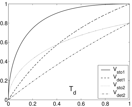
Figure 4: Visibilities of single and double loop interferometers. The visibilities $V_{sto1}$ for stochastic (Eq.(11)) and $V_{det1}$ for deterministic (Eq.(13)) absorption in a single loop interferometer are shown as a function of transmission probability $T_{d}$ in beam path $(d)$. In the double loop interferometer no phase shifter $\Delta_{f}$ and no absorber $\alpha_{f}$ is in beam path $(f)$. In this case the visibilities $V_{sto2}$ and $V_{det2}$ of Eqs.(15) and (17) are smaller than in a single loop device.

An interesting case arises, if a phase shifter $\Delta_{f}$ (and no absorption $\alpha_{f}$) is inserted in beam path $(f)$. The intensity then becomes

$$K_{0}\,{\propto}\,|\,e^{ik_{0}\Delta_{d}-\alpha_{d}}+1+e^{ik_{0}\Delta_{f}}|^{2}=$$

$$=\,T_{d}+2\,\sqrt{T_{d}}{\,}[cos(\Delta_{d}k_{0})+cos(\Delta_{d}k_{0}-\Delta_{f}k_{0})]+4\,cos^{2}(\Delta_{f}k_{0}/2)\,\,\,\,\,.$$ (18)

If $\Delta_{f}=0$, then Eq.(18) reduces to Eq.(14). If $\Delta_{f}k_{0}=(2n+1)\pi$, then $e^{i\Delta_{f}k_{0}}=-1$ and $K_{0}{\propto}T_{d}$. If $2n\pi{\leq}\Delta_{f}k_{0}{\leq}(2n+1)\pi$, maxima of $K_{0}$ are at $\Delta_{d}k_{0}=\Delta_{f}k_{0}/2+2n\pi$ and minima at $\Delta_{d}k_{0}=\Delta_{f}k_{0}/2+(2n+1)\pi$. These maxima and minima are interchanged in the range $(2n+1)\pi{\leq}\Delta_{f}k_{0}{\leq}(2n+2)\pi$, and it is not necessary to consider this case separately. One gets:

$$K_{0,\frac{max}{min}}{\propto}\,T_{d}{\pm}4\,cos(\Delta_{f}k_{0}/2)[\sqrt{T_{d}}{\pm}cos(\Delta_{f}k_{0}/2)]\,\,\,\,\,,$$ (19)

where the upper sign belongs to the maximum and the lower sign to the minimum intensity. The visibility is

$$V_{sto2\Delta_{f}}=\frac{4\,\sqrt{T_{d}}{\,}cos(\Delta_{f}k_{0}/2)}{4\,cos^{2}(\Delta_{f}k_{0}/2)+T_{d}}\,\,\,\,\,.$$ (20)

If $\Delta_{f}k_{0}=0$, then $V_{sto2\Delta_{f}}=V_{sto2}$. If $\Delta_{f}k_{0}=2\pi/3$, then $V_{sto2\Delta_{f}}=V_{sto1}$. In particular we emphasize the fact that the maximum of the function $V_{sto2\Delta_{f}}$ is at $T_{d}=4\,cos^{2}(\Delta_{f}k_{0}/2)$ where $V_{sto2\Delta_{f}}=1$. For a given transmission $T_{d}$ in beam path $(d)$ a phase shift $\Delta_{f}k_{0}=2\,arccos(\sqrt{T_{d}}/2)$ in path $(f)$ should be chosen in order to achieve a visibility of $1$ (Fig.(5) and Fig.(6))! Setting $T_{d}=1$ the relation $V_{sto2\Delta_{f}}$ of Eq.(20) reduces to a formula which already has been discussed in [3] (see Fig.(6)).

An analogous equation can be derived for the deterministic case which reads (Fig.(7))

$$V_{det2\Delta_{f}}=\frac{4\,{T_{d}}{\,}cos(\Delta_{f}k_{0}/2)}{4\,cos^{2}(\Delta_{f}k_{0}/2)+T_{d}}\,<\,1\,\,\,\,\,\,\,,\,\,for\,\,\,\,T_{d}<1\,\,\,.$$ (21)

In case of deterministic visibility the value of $1$ cannot be achieved for $T_{d}<1$.

In order to compare intensities and to assess possibilities for measurements, Figs.(8a,b,c) present values of $K_{0}$ and $K_{G}$ as a function of the phase shift $\Delta_{d}k_{0}$ in beam path $(d)$. From these figures it can be concluded that in spite of strong absorption small signals can be measured with visibility $1$ and with sufficient intensity by adequately adjusting the phase shifter in the second loop of the interferometer. However, as shown in the next section, the described procedure specifies an ideal situation and there is a limit for measuring weak signals using such a technique.

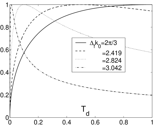
Figure 5: Visibility $V_{sto2\Delta_{f}}$ (Eq.(20)) in a double loop interferometer as a function of transmission probability $T_{d}$ in beam path $(d)$. A phase shift $\Delta_{f}k_{0}$ is applied in beam path $(f)$. The visibility attains the value $1$ for $T_{d}=4\,cos^{2}(\Delta_{f}k_{0}/2)$.

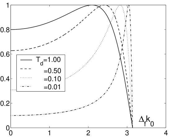
Figure 6: Visibility $V_{sto2\Delta_{f}}$ (Eq.(20)) in a double loop interferometer as a function of phase shift $\Delta_{f}k_{0}$ in beam path $(f)$. A transmission probability $T_{d}$ is applied in beam path $(d)$. The visibility attains the value $1$ for $T_{d}=4\,cos^{2}(\Delta_{f}k_{0}/2)$, where the $4$ parameters $T_{d}$ correspond to those $4$ parameters $\Delta_{f}k_{0}$ in Fig.(5) via this equation.

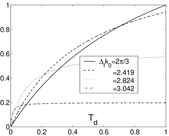
Figure 7: Visibility $V_{det2\Delta_{f}}$ (Eq.(21)) in a double loop interferometer as a function of transmission probability $T_{d}$ in beam path $(d)$. A phase shift $\Delta_{f}k_{0}$ is applied in beam path $(f)$. Contrary to $V_{sto2\Delta_{f}}$ this function $V_{det2\Delta_{f}}$ cannot attain a value of $1$ for $T_{d}<1$.

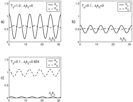
Figure 8: Intensities $K_{0}$ and $K_{G}$ behind the double loop interferometer (see Fig.(1)) as a function of the phase shift $\Delta_{d}k_{0}$ in beam path $(d)$. a) No absorption in beam $(d)$ ($T_{d}=1$) and no phase shift in beam $(f)$ ($\Delta_{f}k_{0}=0$). Fig.(8a) can be compared to Fig.(2). Note that in Fig.(8a) the intensities $K_{0}$ and $K_{G}$ are plotted as a function of $\Delta_{d}k_{0}$. b) Absorption in beam $(d)$ (transmission $T_{d}=0.1$) and no phase shift in beam $(f)$. The intensities have been attenuated accordingly. c) $\Delta_{f}k_{0}=2.824$ has been chosen. This value corresponds to $T_{d}=0.1$ (see Figs.(5) and (6)). $K_{0}$ shows a visibility of $1$ because of $I_{min}=0$.

4 Discussion and conclusion

In this paper some intensity and visibility aspects of a double loop neutron interferometer have been considered. In the first part the wave functions of a triple wave function superposition in the forward and diffracted direction behind the interferometer has been described using the theory of dynamical diffraction in single crystals. Phase shifters and absorbers have been taken into account. In general the intensity levels of the forward and diffracted beams are different. Under certain circumstances these levels can be made equal using various absorbers. This is an interesting new aspect because in this case the device can be regarded as a $50/50$ beam splitter. This feature is not possible in a single loop interferometer.

In the second part the visibility has been investigated. As an another important new result it has been shown that a visibility value of $1$ may be reached when the transmission $T_{d}$ (for stochastic absorption processes) in the first loop is adjusted accordingly to the phase shift $\Delta_{f}k_{0}$ in the second loop:

$$T_{d}=4cos^{2}(\Delta_{f}k_{0}/2)\,\,\,\,\,\,\,{\rightarrow}\,\,\,\,V_{sto2\Delta_{f}}=1.$$ (22)

$T_{d}=e^{-2\alpha_{d}}$ is the transmission probability in beam $(d)$ ($\alpha_{d}$ is the absorption coefficient) and $\Delta_{f}$ is the phase shift in beam $(f)$, where - according to Fig.(1) - the intensity $K_{0}$ in the forward direction behind the double loop interferometer oscillates as a function of the phase shift $\Delta_{d}$ in beam $(d)$. Using the described method in principle every signal in path $(d)$ can be transformed to a signal $K_{0}$ with visibility $1$ and therefore the method could be most interesting for small signals.

It should be noted that to describe real experimental situations an additive term $I_{incoh}$ must be introduced in Eq.(18) to represent the incoherent part of the intensity (background intensity). The main reason for the incoherent effects is non - interference because of crystal imperfection (not absolute parallelism of the crystal lattice planes throughout the interferometer) as well as lattice vibrations and small temperature gradients. The term $I_{incoh}$ leads to a new visibility $V^{{}^{\prime}}_{sto2\Delta_{f}}$:

$$V^{{}^{\prime}}_{sto2\Delta_{f}}=\frac{4\,\sqrt{T_{d}}{\,}cos(\Delta_{f}k_{0}/2)}{4\,cos^{2}(\Delta_{f}k_{0}/2)+T_{d}+I_{incoh}}\,\,\,\,\,.$$ (23)

This expression is always less than $1$ for $I_{incoh}>0$ (see also Eq.(22)). In order to measure weak signals (see Fig.(8c)) the background intensity has to be as small as possible. This could be a serious constraint considering real experimental conditions using neutrons. It should be mentioned that the background intensity has no influence on Eq.(8) concerning the $50/50$ beam splitter system. Note also that an additional empty phase which is a signature of an interferometer does not affect the aforementioned considerations about the intensity and visibility.

It is a common problem in signal processing to measure weak signals. The absorber serves only to generate these signals. In spite of the constraints mentioned above for almost ideal experimental situations Eq.(22) predicts a visibility close to $1$. This could also be the case in systems of Mach - Zehnder interferometers using laser beams. Here the number of counts registered in a detector in a certain time interval obeys a Poisson distribution with variance $(\Delta{N})^{2}=\bar{N}$, where $\bar{N}$ is the mean number of counts. The Poisson distribution is a signature of coherent state behavior. For small count rates the described method may be used to measure small signals with visibility $1$.

The system can easily be adapted (loop $B$ in Fig.(1)) to an eight-port interferometer as a high sensitive homodyne detection setup [4,7,8] as shown in Fig.(9). In this case two vacuum inputs ${\,}|0>{\,}$ have to be added and the strong local oscillator limit can be applied to the idler beam $(a)$ when the signal beam $(e)$ is relatively strongly attenuated by an absorber $\alpha_{e}$. Homodyne detection in laser interferometry is a method, in which the field amplitudes (the quadrature components) are measured instead of the quantized intensity. The balanced version of homodyne detection has a great practical advantage of cancelling technical noise and the classical instabilities of the reference field. Thereby the signal interferes with a coherent laser beam at a well-balanced $50/50$ beam splitter. It provides the phase reference for the quadrature measurement. The intensity difference is the quantity of interest because it contains the interference term of the local oscillator and the signal.

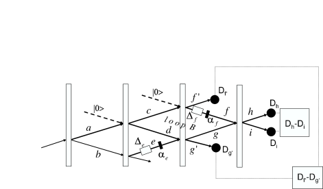
Figure 9: An eight-port interferometer is built up from loop $B$ in Fig.(1). Neutron count rate differences can be measured by the detectors $D_{h}$ and $D_{i}$ as well as $D_{f^{\prime}}$ and $D_{g^{\prime}}$. The phase of the strongly attenuated signal beam (e) can be modified by a phase shift $\Delta_{e}$. The strong local oscillator is given by the idler beam (a).

Finally, as already mentioned above, we would like to point out again that there are good reasons to assume that a similar result can be attained in double Mach-Zehnder interferometry where photonic beams in fiber glass are used. As a visibility near to $1$ is of great advantage for measuring largely attenuated beams, our approach outlines a general method to investigate weak signals in double loop interferometric devices.

References