The spectrum of a quantum potential

Abstract

We apply a method recently devised by one of the authors to obtain precise analytical formulas for the spectrum of quartic and sextic anharmonic potential. Due to its general features the method can be applied with minimal effort to a wide class of quantum potentials thus allowing very promising applications.

Recently one of the authors has developed a method which allows to obtain analytical approximations to a certain class of integrals with arbitrary precision [1, 2]. It has been proven that the expansion proposed in [1] converges uniformly and that it yields excellent results already to first order. Such method has been applied to a large class of problems in Classical Mechanics and General Relativity, allowing to obtain simple analytical formulas which work even in the non-perturbative regime.

In this letter we deal with a further application of the method, showing that it is possible to obtain accurate analytical expressions for the spectrum of a quantum potential by using it in conjunction of the WKB expansion. Although our calculations are obtained for the anharmonic potential, the procedure that we suggest applies with minor changes to any potential.

We will use [3] as our main reference: in that paper Bender and collaborators show how to solve the one-dimensional eigenvalue problem for analytic potential to all orders in the WKB approximation. They obtain a recursion relation for the WKB corrections and they are able to sum the WKB series in two special cases, recovering the exact energy eigenvalues.

However, in the general case of a potential $V(x)$ the calculation of the WKB correction to a given order can be difficult and, depending on the potential itself, it is possible that no analytical expression can be found for the WKB integrals. By applying the method of [1] to the anharmonic oscillator to order $\hbar^{4}$ we show that one can obtain a precise analytical approximation to the entire spectrum of the potential. The precision of the approximation depends both on the order to which the WKB expansion is considered and on the order to which our method is applied.

Let us briefly review the method by considering the integral ${\cal J}_{1}=\int_{x_{-}}^{x_{+}}\ \sqrt{E-V(x)}\ dx$. $x_{\pm}$ are the classical turning points of the potential $V(x)$ and $E=V(x_{\pm})$ is the energy. In the spirit of the Linear Delta Expansion [4] we interpolate the potential $V(x)$ as

$$V_{\delta}(x)=V_{0}(x)+\delta\ (V(x)-V_{0}(x))\ ,$$ (1)

where $V_{0}(x)$ is a potential introduced by hand, which depends on one or more arbitrary parameters. $V_{\delta}(x)$ reduces to the full potential for $\delta=1$. We want to perform an expansion described by eq. (1) without moving the inversion points; for this reason we ask that $x_{\pm}$ be the inversion points also of the potential $V_{0}(x)$. As a result, the energy $E_{0}$ that the particle would possess if it was moving only in the potential $V_{0}(x)$ will be given by:

$$E_{0}=V_{0}(x_{\pm})\ .$$ (2)

We therefore write the integral as

$${\cal J}_{1} = \int_{x_{-}}^{x_{+}}\ \sqrt{E_{0}-V_{0}(x)}\ \left[1+\delta\Delta(x)\right]^{1/2}\ dx$$ (3)

where

$$\Delta(x)\equiv\frac{E-E_{0}-V(x)+V_{0}(x)}{E_{0}-V_{0}(x)}.$$ (4)

We treat the term proportional to $\delta$ as a perturbation and perform an expansion in $\delta$. Such expansion will converge uniformly when $|\Delta(x)|<1$ in the region $x_{-}\leq x\leq x_{+}$ [1]. This condition selects a particular region in the parameter space, i.e. $\lambda$; however, maximal convergence is achieved when the Principle of Minimal Sensitivity (PMS) [5] is used, i.e. when the condition $d{\cal J}_{1}/d\lambda=0$ is enforced. Notice that if the potential $V_{0}(x)$ is chosen appropriately it will be possible to calculate analytically each term in the expansion.

We now come explicitly to the WKB integrals. We perform our analysis to order $\hbar^{4}$ and use the recursion formulas of [3] to calculate the spectrum of the anharmonic oscillator. Following [6] we write the integral in a fashion where the singularities in the integrand are integrable. The price that we pay is that we have to introduce derivatives with respect to the energy.

We therefore write the WKB condition as

$$\Lambda(E)=\frac{\pi\hbar}{\sqrt{2m}}\ (n+1/2)$$ (5)

where $\Lambda(E)$ to order $O(\hbar^{6})$ is given by

$$\Lambda(E) \equiv {\cal J}_{1}(E)-\frac{\hbar^{2}}{48\ m}\frac{d}{dE}{\cal J}_{2}(E)+\frac{\hbar^{4}}{11520\ m^{2}}\frac{d^{3}}{dE^{3}}{\cal J}_{3}(E)\ .$$ (6)

We have defined:

$${\cal J}_{1}(E) \equiv \int_{x_{-}}^{x_{+}}\sqrt{E-V(x)}dx$$ (7)

$${\cal J}_{2}(E) \equiv \int_{x_{-}}^{x_{+}}\frac{V^{\prime\prime}(x)}{\sqrt{E-V(x)}}dx$$ (8)

$${\cal J}_{3}(E) \equiv \int_{x_{-}}^{x_{+}}\frac{7\ V^{\prime\prime}(x)^{2}-5\ V^{\prime}(x)\ V^{\prime\prime\prime}(x)}{\sqrt{E-V(x)}}dx$$ (9)

where $x_{\pm}$ are the classical turning points. The spectrum of the potential $V(x)$ can be obtained by solving Eq. (6).

So far we have used general formulas; let us consider now the specific case of the anharmonic oscillator $V(x)=\frac{m\omega^{2}x^{2}}{2}+\frac{\mu x^{4}}{4}$. We choose the interpolating potential $V_{0}(x)=\frac{1}{2}\left(m\omega^{2}+\lambda^{2}\right)\ x^{2}$. The method of [1] allows to calculate the integrals in Eq. (6) quite simply. Indeed to order $\delta^{10}$ and using the value of $\lambda$ obtained by the PMS to first order one obtains:

$${\cal J}_{1}(\zeta) = \frac{m^{3/2}\ \pi\ \omega^{3}}{\mu\ \zeta^{\frac{3}{2}}\ \left(5+8\ \zeta\right)^{\frac{19}{2}}}\ \sum_{n=0}^{10}\ c_{n}^{(1)}\ \zeta^{n}$$ (10)

$${\cal J}_{2}(\zeta) = \frac{{\sqrt{m}}\ \pi\ \omega\ {\left(3+2\ \zeta\right)}^{\frac{3}{2}}}{{\sqrt{\zeta}}\ {\left(21+36\ \zeta+16\ {\zeta}^{2}\right)}^{\frac{21}{2}}}\ \sum_{n=0}^{20}\ c_{n}^{(2)}\ \zeta^{n}$$ (11)

$${\cal J}_{3}(\zeta) = \frac{m^{\frac{3}{2}}\ \pi\ \omega^{3}\ {\left(99+48\ \zeta+56\ {\zeta}^{2}\right)}^{\frac{3}{2}}}{{\sqrt{2}}\ {\zeta}^{\frac{3}{2}}\ {\left(363+564\ \zeta+360\ {\zeta}^{2}+224\ {\zeta}^{3}\right)}^{\frac{21}{2}}}\ \sum_{n=0}^{30}\ c_{n}^{(3)}\ \zeta^{n}$$ (12)

where we have introduced the variable $\zeta\equiv\frac{m\ \omega^{2}}{\mu\ A^{2}}$ and $x_{\pm}=\pm A$ are the classical turning points. The coefficients $c_{n}^{(i)}$ are pure numbers, which we will not display here.

In Fig. 1 we plot the error defined as $\Xi_{i}=\left|\frac{{\cal J}_{i}^{(\delta)}-{\cal J}_{i}^{(exact)}}{{\cal J}_{i}^{(exact)}}\right|\ \times 100$ as a function of the energy. We exploit the relation between the amplitude and the energy, i.e. $E=V(A)$, to express $\zeta$ as a function of the energy:

$$\zeta=\frac{m^{2}\omega^{4}}{4\mu E_{n}}\ \left[1+\sqrt{1+\frac{4\mu E_{n}}{m^{2}\omega^{4}}}\right]\ .$$ (13)

${{\cal J}_{i}^{(exact)}}$ are the exact integrals. We have assumed the values $m=\omega=\hbar=\mu=1$.

We observe that the error is smaller at lower energies and flattens around values of the order of $10^{-5}$ at large energies. Such result can be further improved by applying our method to higher orders in $\delta$: indeed it was proved in [1] that the method is convergent and therefore the precision of the calculation can be easily improved. We stress that the behavior of this error is somewhat complementary to the one expected for the WKB expansion, which is known to work better for the highly excited states. This is of course a nice feature, which allows to obtain a higher precision in our calculations.

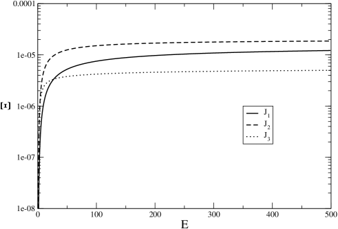
Figure 1: Error over the integral ${\cal J}_{i}$ for $m=\omega=\hbar=\mu=1$ as a function of the energy.

Once Eqs. (10), (11) and (12) are substituted back in Eq. (6) one obtains a rather complicated expression, which still needs to be inverted in order to give the energy as a function of the quantum number $n$. However this task is easily accomplished by Taylor expanding Eq. (6) around $\zeta=0$ (which corresponds to the higher part of the spectrum) and by then using eq. (13).

We obtain the approximate analytical formula for the spectrum of the quartic anharmonic oscillator:

$$E_{n} \approx e_{1}\ \left(n+\frac{1}{2}\right)^{\frac{4}{3}}+e_{2}\ \left(n+\frac{1}{2}\right)^{\frac{2}{3}}+e_{3}+\frac{e_{4}}{\left(n+\frac{1}{2}\right)^{2/3}}+\dots$$ (14)

where the first few coefficients $e_{i}$ are given by

$$e_{1} = \frac{8192000000000000\,{\left(\frac{2}{371496873}\right)}^{\frac{1}{3}}\,5^{2/3}}{48413843986233}\ {\left(\frac{{\mu}\ {{\hbar}}^{4}}{m^{2}}\right)}^{\frac{1}{3}}\approx 0.867146\ {\left(\frac{{\mu}\ {{\hbar}}^{4}}{m^{2}}\right)}^{\frac{1}{3}}$$ (15)

$$e_{2} = \frac{223553096351603200000\,{\left(\frac{2}{371496873}\right)}^{2/3}\ 5^{1/3}}{2759589107215281}\ \left(\frac{\hbar\ m}{\sqrt{\mu}}\right)^{2/3}\ \omega^{2}$$ (16)

$$\approx 0.42551\left(\frac{\hbar\ m}{\sqrt{\mu}}\right)^{2/3}\ \omega^{2}$$

$$e_{3} = -\frac{22736856054709769417272276}{486959893945285848925248675}\ \frac{m^{2}\ \omega^{4}}{\mu}\approx-0.0466914\ \frac{m^{2}\ \omega^{4}}{\mu}$$ (17)

$$e_{4} = \frac{9339788533820875\,5^{\frac{1}{6}}}{131900122669056\,2^{\frac{2}{3}}\,{\sqrt{7}}\,{371496873}^{\frac{1}{3}}}\ \left(\frac{\mu\hbar^{4}}{m^{2}}\right)^{1/3}$$ (18)

$$+ \frac{8271957929254630511939617633398178757}{999241702375726561994610281100000000\,2^{\frac{2}{3}}\,{1857484365}^{\frac{1}{3}}}\ \left(\frac{m^{10}\omega^{6}}{\mu^{5}\hbar^{2}}\right)^{1/3}$$

$$\approx 0.030669\left(\frac{\mu\hbar^{4}}{m^{2}}\right)^{1/3}+0.00424238\ \left(\frac{m^{10}\omega^{6}}{\mu^{5}\hbar^{2}}\right)^{1/3}\ .$$

Notice that altough the coefficients $e_{i}$ of higher order could be calculated as well, it is not necessary to do so, since they would only provide corrections that would be dominated by the error that we are making evaluating the integrals ${\cal J}_{i}$.

In Fig. 2 we plot the energy eigenvalues of the last column of Table III of [7], corresponding to $\hbar=1$, $m=1/2$, $\omega=2$ and $\mu=8000$ and compare them with the approximate results obtained by using eq. (14). It is clear that our formula, although quite simple, works excellently.

In Fig. 3 we display the error over the energy defined as $\Sigma\equiv\left|\frac{E_{n}^{(approx)}-E_{n}^{(exact)}}{E_{n}^{(exact)}}\times 100\right|$ as a function of the quantum number $n$. The boxes have been obtained using our formula eq. (14) and assuming $\hbar=1$, $m=1/2$, $\omega=2$ and $\mu=8000$. In this case $E_{n}^{(exact)}$ are the energies of the anharmonic oscillator calculated with high precision in last column of Table III of [7]. The jump corresponding to $n=25$ is due to the low precision of the last value of Table III of [7]. The pluses and the triangles have been obtained using our formula eq. (14) (pluses) and eq. (1.34) of [8] (triangles) and assuming $\hbar=m=\omega=1$ and $\mu=4$. In this case $E_{n}^{(exact)}$ are the energies of the anharmonic oscillator numerically calculated through a fortran code. We can easily appreciate that our formula provides an approximation which is several order of magnitude better than the one of eq. (1.34) of [8].

As a further check on the soundness of our approximation we consider the quantum zeta function for the quartic anharmonic oscillator [9, 10]:

$$Z(s)=\sum_{n=0}^{\infty}\frac{1}{E_{n}^{s}}$$ (19)

The exact value of $Z(1)$ corresponding to setting $\omega=0$ and $\mu=4$ is known to be

$$Z(1)=\frac{3^{2/3}}{8\pi^{2}}\Gamma^{5}\left(\frac{1}{3}\right)\approx 3.63500364488\ .$$ (20)

We have estimated $Z(1)$ by using the first few numerical eigenvalues and then using for the remaining ones the analytical formula corresponding to the solution of eq. (14). Using our formula eq. (14) only taking the first $4$ eigenvalues numerically we have obtained the value

$$Z_{4}(1)=3.635002$$ (21)

which can be compared with the value

$$Z_{140}(1)=3.6350017$$ (22)

obtained in [10] by using a much larger set of numerical eigenvalues.

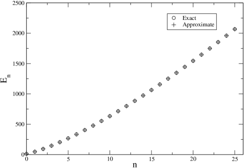
Figure 2: Comparison between the numerical eigenvalues of [7] and the results obtained using eq. (14). We assume $\hbar=1$, $m=1/2$, $\omega=2$ and $\mu=8000$.

Figure 3: Error over the energy of the anharmonic oscillator with $\hbar=1$, $m=1/2$, $\omega=2$ and $\mu=8000$ (set 1) and with $\hbar=m=\omega=1$ and $\mu=4$ (set 2). The boxes and the pluses have been obtained with our method, the triangles correspond to the error calculated using the analytical formula of [8].

We have also applied our method to the case of a anharmonic potential of the form $V(x)=\omega x^{2}/2+\rho x^{6}/6$. In this case we have used the WKB expansion to leading order and we have approximated with our method the integral ${\cal J}_{1}$ corresponding to this potential. In Fig. 4 we display the error $\Xi=\left|\frac{{\cal J}_{1}^{(\delta)}-{\cal J}_{1}^{(exact)}}{{\cal J}_{1}^{(exact)}}\right|\ \times 100$ as a function of the energy. ${\cal J}_{1}^{(exact)}$ is the exact value of the integral calculated numerically, whereas ${\cal J}_{1}^{(\delta)}$ is the analytical approximant obtained with our method to order $10$. Although the error increases with the energy, we notice that it is always smaller than $0.01\%$. As in the case of the quartic oscillator, our approximation works better in the region of low energy, i.e. opposite to the WKB method.

By using the approximation for the integral ${\cal J}_{1}$ obtained with our method we have derived a very simple formula for the spectrum of the sextic oscillator to leading order in the WKB expansion:

$$E_{n} = \frac{1}{\left(\alpha_{1}\left(n+\frac{1}{2}\right)+\alpha_{2}-\sqrt{\beta_{1}\left(n+\frac{1}{2}\right)^{2}+\beta_{2}\left(n+\frac{1}{2}\right)+\beta_{3}}\right)^{3/2}}$$ (23)

where

$$\alpha_{1} = \frac{20887573200705159168\,6^{\frac{1}{6}}\,{\sqrt{11}}\,{\hbar}\,\,{\rho}^{\frac{5}{6}}}{5057378805833647189\,m^{\frac{5}{2}}\,\omega^{4}}\approx 18.46505979\ \frac{\hbar\rho^{5/6}}{m^{5/2}}$$

$$\alpha_{2} = \frac{8129630071150442107\,6^{\frac{2}{3}}\,{\rho}^{\frac{1}{3}}}{5057378805833647189\,m\,\omega^{2}}\approx 5.307778611\ \frac{\rho^{1/3}}{m\omega^{2}}$$

$$\beta_{1} = \frac{4799197856362980042268993891174358974464\,6^{\frac{1}{3}}\,{{\hbar}}^{2}\,{\rho}^{\frac{5}{3}}}{255770803856953672746878259\ 25727601721\,m^{5}\,\omega^{8}}$$

$$\approx 340.9584332\ \frac{\hbar^{2}\rho^{5/3}}{m^{5}\omega^{8}}$$

$$\beta_{2} = \frac{339616486411617501798889917918008573952\,6^{\frac{5}{6}}\,{\sqrt{11}}\,{\hbar}\,{\rho}^{\frac{7}{6}}}{255770803856953672\ 74687825925727601721\,m^{\frac{7}{2}}\,\omega^{6}}$$

$$\approx 196.0168989\frac{\hbar\rho^{7/6}}{m^{7/2}\omega^{6}}$$

$$\beta_{3} = -\frac{177921136833163170599693588290032640752\,6^{\frac{1}{3}}\ {\rho}^{\frac{2}{3}}}{25577080385695367274687825925727601721\,m^{2}\,\omega^{4}}$$

$$\approx -12.64038572\frac{\rho^{2/3}}{m^{2}\omega^{4}}\ .$$

In Fig. 5 we compare the lower part of the spectrum obtained using eq. (23) with the exact eigenvalues, obtained numerically with a fortran code. Once again the agreement between the two is impressive. Fig. (6) displays the error (in $\%$) over the energy obtained using eq. (23). The error is of the order of a few percents for low values of $n$, but drops quite quickly, reaching a plateau of about $0.01\%$ at large $n$. The presence of the plateau is a consequence of the error that we are making in the evaluation of ${\cal J}_{1}$, as already discussed when we considered Fig. 4. Since the method that we are using is convergent[1, 2], by working to higher orders one can arbitrarily lower the position of such plateau, to obtain the highly excited part of the energy spectrum with the desired accuracy.

Figure 4: Error over the integral $J_{1}$ for $\hbar=m=\omega=\rho=1$.

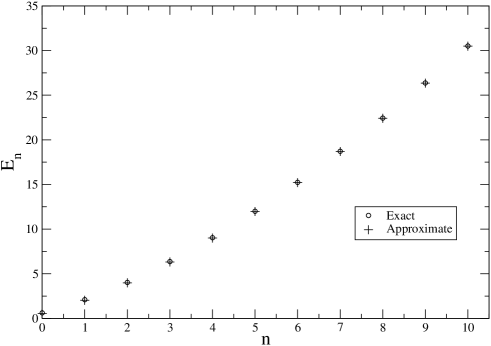
Figure 5: Lower part of the spectrum of the sextic anharmonic oscillator. The circles are the exact eigenvalues calculated numerically and the pluses are the results of eq. (23). We assume $\hbar=m=\omega=\rho=1$.

Figure 6: Error over the energy obtained using eq. (23) and assuming $\hbar=m=\omega=\rho=1$.

In conclusion we have shown that the method of [1, 2] can be easily applied to calculate fully analytical expressions for the energy spectrum of quantum potentials within the WKB approximation. By applying our method to a sufficiently large order in $\delta$ we are able to estimate analytically the WKB integrals with high precision, given the convergent nature of the expansion that we are performing. The application of this method to more general potentials in $1$ and $3$ dimensions is currently underway.

References

References

• [1] Amore P and Sáenz R A, Preprint math-ph/0405030
• [2] Amore P, Aranda A, Fernández F M and Sáenz R A, Preprint math-ph/0407014
• [3] Bender C M, Olaussen K and Wang P S, Phys. Rev. D 16 (1977) 1740
• [4] A. Okopińska, Phys. Rev. D 35, 1835 (1987); A. Duncan and M. Moshe, Phys. Lett. B 215, 352 (1988)
• [5] P. M. Stevenson, Phys. Rev. D 23, 2916 (1981).
• [6] Dobrovolsky G A and Tutik R S, Journal of Physics A 33 (2000) 6593
• [7] H. Meissner and O. Steinborn, Phys. Rev. A 56, 1189 (1997).
• [8] Feranchuk I. D., Komarov L. I., Nichipor I. V. and Ulyanenkov A.P., Annals of Physics 238 370 (1995)
• [9] A. Voros, Nuclear Physics B 165 (1980) 209
• [10] R. E. Crandall, Journal of Physics A 29 (1996) 6795