Diffraction and trapping in circular lattices
Abstract
When a single two-level atom interacts with a pair of Laguerre-Gaussian beams with opposite helicity, this leads to an efficient exchange of angular momentum between the light field and the atom. When the radial motion is trapped by an additional potential, the wave function of a single localized atom can be split into components that rotate in opposite direction. This suggests a novel scheme for atom interferometry without mirror pulses. Also atoms in this configuration can be bound into a circular lattice.
I Introduction
It is well-known that light may carry both angular and linear momentum. When a light field interacts with matter, exchange of momentum and angular momentum between light and matter can occur. Laguerre-Gaussian (LG) light modes are known to carry orbital angular momentum. If one employs the paraxial approximation for the light field, simple expressions for the field amplitudes and its average angular momentum can be derived [1]. An easy way to produce such beams is using spiral phase plates [2].
Another important question is the separability of the total angular momentum into ’orbital’ and ’spin’ parts [3]. The orbital part is associated with the phase distribution of the light field, and the spin part is connected with its polarization. This question is essential in the context of momentum transfer from light to the atom when one includes atomic internal degrees of freedom. It has been shown that ’spin’ and ’orbital’ angular momentum of the photon are transferred from the quantized light field to, respectively, the internal and the external angular momentum of the atom. The interaction with a LG mode is a possible way to entangle internal and external degrees of freedom of an atom [4]. The transfer of the angular momentum of light to particles has been also experimentally demonstrated in [5], where trapped massive particles are set into rotation while interacting with the light field. Other authors have studied the cooling properties for atoms using LG beams [6]. Also LG beams have been proposed as a trapping potential for Bose condensates [7].
Whereas angular momentum exchange between light and matter is a relatively new topic, the linear momentum exchange is a well-established issue [8]. It is well-known that two counterpropagating waves lead to a more efficient exchange of linear momentum between an atom and the light field than a single travelling wave. Using quantum language for a classical light field, one can describe such an interaction as a sequence of successive single photon absorption and emission events. This suggests that one may expect more efficient angular momentum exchange between a light field and an atom if one uses two LG modes with opposite helicity, e.g. counterrotating waves.
II General framework
We start with radiation fields propagating along the -axis with wave number and carrying orbital angular momentum (Laguerre-Gaussian beams). If one considers the paraxial limit of these waves, the expressions for the light fields are particularly simple [1]
| (1) |
where are the cylindrical coordinates, is the frequency and the integer index is indicates the helicity of the LG beam. For two Laguerre-Gaussian beams with opposite helicity, namely and , the total field can be written as
| (2) |
We indicated already in the Introduction, that one expects a more efficient exchange of angular momentum between the light field and the atom in the configuration (2) than in a single LG mode. This expectation is based on the corresponding situation of momentum exchange between an atom and a standing light wave. In addition to the light field (2), the atomic motion in the radial direction is assumed to be confined by an extra trapping potential with cylindrical symmetry.
The dependence of the amplitude is slow and can be ignored. Properly shaping the LG mode, the radial dependence of can be ignored on the characteristic width of the trapping potential . Thus, we assume that is constant. For a two-level atom the Hamiltonian in the rotating-wave approximation can then be written as
| (3) |
where is the Rabi frequency of each of the travelling waves that create the standing wave, is the laser frequency, and
| (4) |
is the Hamiltonian for a free atom, with the momentum operator of the atom, and indicate the ground and excited states, and defines the transition frequency of a free atom.
The dynamics of the atom is rather simple if the laser is far detuned. We assume that
| (5) |
where the detuning is defined as For an atom in the ground state, the excited state can be adiabatically eliminated, which leads to an effective Hamiltonian in the well-known form
| (6) |
where the light-shift potential is specified by
| (7) |
with
III Trapping in counterrotating fields
Some general conclusions on the bound states of the Hamiltonian (6) directly follow from its symmetry properties. We introduce the unitary translation operator defined as
| (8) |
where indicates the states with fixed azimuthal angle. Since the Hamiltonian (6) is invariant for rotation about an angle , it follows from a rotational version of the Bloch theorem that the eigenstates of this Hamiltonian are also eigenstates of . The eigenvalue relation can be expressed as
| (9) |
where is referred to as angular quasimomentum and identifies the energy band. We consider a single energy band, and we suppress the index . We can restrict to the first Brillouin zone given as
| (10) |
The eigenstates should be periodic in with period , because a rotation over must leave the wave function invariant. The finite range of leads to a discretization of angular quasimomentum. On the other hand, a rotation over is equivalent to the action of the operator . Since it follows from Eq. (9) that
we conclude that the only possible values of the angular quasimomentum are determined from the condition
Hence must be integer, and each band contains Bloch states. For example, for the first Brillouin zone contains only the four values of the angular quasimomentum.
Also, in analogy to the case of an infinite linear lattice, one can introduce localized Wannier states in the usual manner, as Fourier transforms of the Bloch states
Obviously, the number of Wannier states within an energy band is equal to , just as the number of Bloch states.
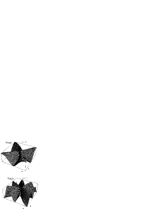
In Fig. 1 we plot the trapping potential (7) for in Cartesian coordinates. When the potential is sufficiently deep, atoms can be bound in the angular wells, and the Wannier states are confined to a single well. An additional confining potential is required to trap particles in the radial direction, and to avoid their escape. Then the potential (7) can create a circular lattice, where particles are located near the minima of the periodic potential. A circular optical lattice has many applications, as discussed recently by several authors [11].
IV Diffraction in counterrotating fields
Since the potentials have a cylindrical symmetry, it is convenient to express the kinetic energy in cylindrical coordinates, and we write
| (11) |
The dynamics along the axis is completely free. For simplicity, we assume that the radial potential is narrow, so that the radial motion is restricted to a ring with radius , and we ignore radial dispersion in the present Section. We return to it in Sec. VI, where the effect of the radial dispersion is estimated. The motion of an atom in the angular direction is then described by the one-dimensional Hamiltonian
| (12) |
which has the azimuthal angle as the only coordinate. The quantity is the moment of inertia. This Hamiltonian is the circular counterpart of the Hamiltonian for simple linear diffraction. The main difference is that the coordinate is periodic, which forces the angular wave number to be integer. Diffraction of a single atom described by such a linear Hamiltonian has been extensively studied theoretically and experimentally by several groups [8].
Just as is usually done for linear diffraction, we consider the situation that an initially localized atom interacts with the optical potential during a small interaction interval , where the atom picks up momentum from the lattice. The transition from the near field immediately after the interaction and the far field is described by free evolution. We assume the atom to be initially in its ground state and situated in a small segment of the ring. Since the angular wave function of the atom must be periodic at all times, we cannot represent a localized wave packet by a Gaussian. The initial state at the beginning of the interaction interval is taken as
| (13) |
with to be a large natural number, and is the normalization constant
| (14) |
The state (13) can be written as a Fourier series, which is just an expansion in the angular-momentum eigenstates. This gives
| (15) |
with
| (16) |
The initial state (13) is localized around , which is clear from the asymptotic form
| (17) |
for large . The half width in the azimuthal angle is of the order of . From the asymptotic form of the binomial coefficient
we find the asymptotic expression of the Fourier coefficient
| (18) |
This demonstrates that the half width in angular momentum is of the order of .
If we take the duration of the light pulse short and the moment of inertia is large, so that , no propagation occurs, and the kinetic-energy term can be neglected during the interaction. This is the equivalence of the standard Raman-Nath approximation applied by Cook et al [10]. Then the final state at time after the interaction is
| (19) |
This state can be expressed as an expansion in angular-momentum eigenstates, in the form Fourier series, which is just an expansion in the angular-momentum eigenstates. This gives
| (20) |
where
| (21) |
in terms of the ordinary Bessel functions.
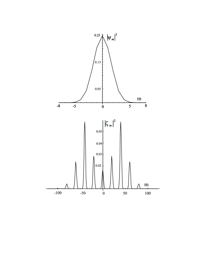
States with large angular momentum are initially not populated, whereas all angular momentum states get populated after the interaction. Thus, the configuration with two LG modes leads to more efficient exchange between the light field and the atom than a single LG beam. The physical interpretation is the same as for diffraction in the field of classical counterpropagating waves: an atom picks up a photon from the light beam with one helicity and emits a photon into the opposite one. In figure 2 we present a typical diffraction pattern calculated for the case that More precisely, we plot the angular-momentum coefficients before the interaction, and the coefficients after the interaction with the circular lattice, for In the latter case, the momentum peaks correspond to different values of . The distance between neighboring peaks is equal to . The half width of each peak is of the order of
V Free evolution on a ring
As shown above, the angular-momentum distribution of an atom after the interaction with a pair of counterrotating LG beams can be broad. However, as a result of the Raman-Nath approximation, the angular distribution of the atom has not been modified during the interaction, so that . In this chapter we investigate the spatial form of the atomic distribution in the far field, i. e. after free evolution of the atom over the ring. As before, the motion along the axis is completely free and the radial motion is restricted on a ring. The initial state of this free evolution is given by Eq. (19), with the expansion in angular-momentum states given by Eqs. (20) and (21). For positive times, the atomic motion is still restricted to the ring with radius by the confining potential , and the evolution of the angular wave function is governed by the Hamiltonian (12) with . With the initial state (20), the time-dependent wave function is given by the expansion
| (22) |
where , and the coefficients are given in Eq. (21). As displayed in Fig. 2, the distribution typically separates in a number of peaks centered at , where which are separated by . Thus, the superposition state (22) can be considered as a series of elementary wave packets centered at in the angular-momentum space. Each of these peaks gives a separate contribution to the wave function that moves with its own angular group velocity . The angular separation between neighboring wavepackets is given by , which is proportional to Since wave packets with opposite angular-momentum values will move in opposite directions, i. e. clockwise and anticlockwise, they will eventually meet again at some time and start to interfere.
In order to estimate the time value that interference sets in, we use the fact that for not too small arguments the Bessel function with the maximal value is the one with . Hence, the meeting time of the pair of the strongest counterpropagating packets is
The exact expression for the time-dependent wave function can be expressed in an integral form by using the mathematical identity [9]
| (23) |
which can be checked by performing the integration. When substituting this identity in the right-hand side of Eq. (22), and using the expansion (20), we arrive at the exact expression
| (24) |
A similar equation is well-known to describe the free evolution of a quantum particle in one dimension. In the present case it is crucial that the integration be performed over all values of , while using that the wave function is periodic. Because of this periodicity, we can express the integral in (24) as a sum of bounded integrals
| (25) |
By a shift of variables the integrations can be performed over the interval , which leads to an integral expression over a single interval
| (26) |
Here we introduced the modified wave function which is just the initial wave function, modified by a phase factor, defined by
| (27) |
In order to emphasize its physical significance, we write Eq. (26) in the form
| (28) |
where the function is the Fourier transform of the modified wave function defined over a single period
| (29) |
For a freely evolving quantum particle in one dimension, the time-dependent wave function has the same form as the term with in (28). The other terms can be understood from the periodic nature of the dynamics on the circle, where each period of the initial wave function serves as an additional source that contributes to the wave function in the relevant interval . Because of the finite range of the integration in Eq. (29), the distinction between the modified wave function and the initial wave function vanishes for times obeying the inequality , when we find in a good approximation
| (30) |
In this limit, the function is just the Fourier transform of the initial wave function , and is simply determined by the Fourier transform of the initial wave function multiplied by a phase factor. The equation (28) has the flavor of the far-field picture of the time-dependent wave function. The Fourier transform of the initial state determines not only the momentum wave function, but also the asymptotic form of the coordinate wave function, scaled by a factor that varies linearly with time. Characteristic for the present case of evolution on a circle is that each interval of length serves as a separate source, each giving a contribution to . Since the Fourier transform of the wave function determines the angular-momentum amplitudes, we may conclude that the wave function for not too small times has the same form as the initial distribution of angular momentum, scaled by the factor .
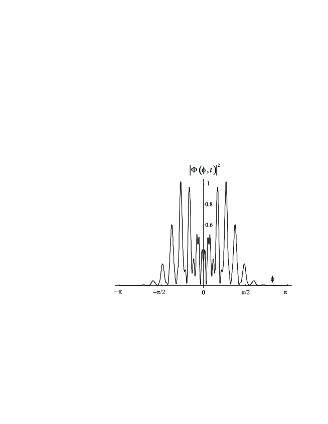
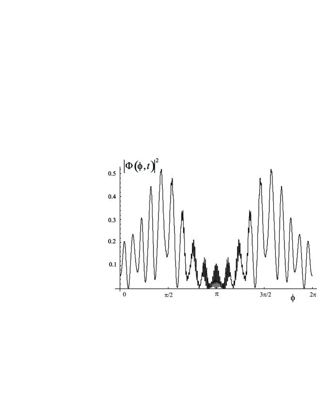
It is clarifying to follow the temporal evolution of by distinguishing two time regions, namely and In the region , the wave function has not yet spread beyond a single period of length , and only a single term in eq. (28) (or (26)) differs from zero. The contribution to the wave function coming from different sources do not overlap yet, so that one can neglect the interference term between them. At later times the diffraction pattern on the interval is formed as an interference pattern between two and more terms in the superposition state (25). This picture is confirmed by numerical calculation of the diffraction pattern for the two time regimes. In Fig. 3 the angular probability distribution is shown for a time . The spatial pattern resembles the angular momentum distribution shown in Fig. 2. Figure 4 displays the same probability distribution for a later time . One notices that the counterrotating components give rise to clear interference fringes. These fringes will be quite sensitive to any perturbation in one of the arms. This suggests to use the present scheme as an atomic interferometer [9]. Usually, interferometers have two key components, namely a beam splitter and a mirror. A coherent incoming atomic beam is split into spatially separated components by the beam splitter. Two arms are getting formed, which freely propagate and may undergo different phase shifts, which are probed by recombining the two arms. The interference pattern contains the information of the phase perturbation in one of the arms. Recombination usually requires atomic mirrors. In atom optics, beam splitters and mirrors are commonly realized by using light pulses, with carefully selected duration and shape.
In the present case, only a single pulse is required that splits the initial atomic wave packet into components rotating to the left and to the right. No mirrors are employed in this scheme. Instead, one uses the radial potential , to constrain the atomic motion to a ring. Radial potentials can be realized by hollow light beams, which are widely used in atomic interferometric schemes.
VI Radial dispersion
In this chapter we consider the radial dynamics of the diffracted wave function during its free evolution, after the passage of the circular lattice. We assume that the wave function at time , after the diffracting pulse, is factorized as
| (31) |
where the radial part of the wave function is sharply peaked at , and the angular wave function is specified by Eq. (20). The radial function is normalized (). We wish to study the possible deformation of the wave packet, when the radial dispersion is included during the stage of free evolution. We take the simplest possible trapping potential, which allows radial dispersion, and we take for the confining potential an infinitely deep cylindrical box with radius , as defined by
| (32) |
This potential models a hollow light beam. With this potential, the normalized eigenfunctions of the Hamiltonian for the cylindrical coordinates during the free-evolution stage take the form
| (33) |
where the radial functions are solutions of the equation
| (34) |
with are the corresponding eigenenergies. The radial functions are proportional to the Bessel function of order
| (35) |
with normalized in the interval . In order that the wave function vanishes at the edge of the cylindrical well, we have to take the numbers for various values of as the subsequent zero’s of the Bessel function . This determines the corresponding eigenenergies as
| (36) |
with . For each value of the angular momentum , the set of functions is complete. An expansion of the initial state (31) in the energy eigenfunction is found when we expand the initial radial wave function in the radial eigenfunctions (35), so that
| (37) |
while substituting Eq. (20) for the initial angular state . For the time-dependent state we find
| (38) |
where the -dependent radial wave function is
| (39) |
¿From Eq. (37) one notices that , independent of the angular momentum . It is obvious from the radial Schrōdinger equation (34) and the initial condition (31) that the normalized radial wave function obeys the identity for all . Moreover, since the total wave function before diffraction is even in , it must remain even for all times. This implies that for all . So just as discussed in Sec. IV, the angular distribution separates in different wave packets that are counterrotating. Since the phase of is even in , its derivative with respect to will be odd, and the angular group velocities of packets with opposite values of will be opposite. This leads to interference after the packets have traversed the entire ring. The initial radial function is taken as a narrow Gaussian
| (40) |
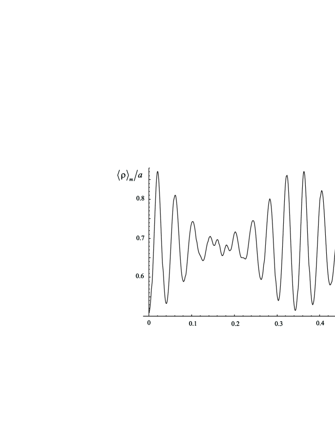
Here is the width and represents the initial position of the wave packet within the box. The normalized wave function describes the radial dynamics for each value of the angular momentum . As an example, we evaluate the time behavior of the average radius for each angular momentum, with the given initial radial state (40), according to the expression
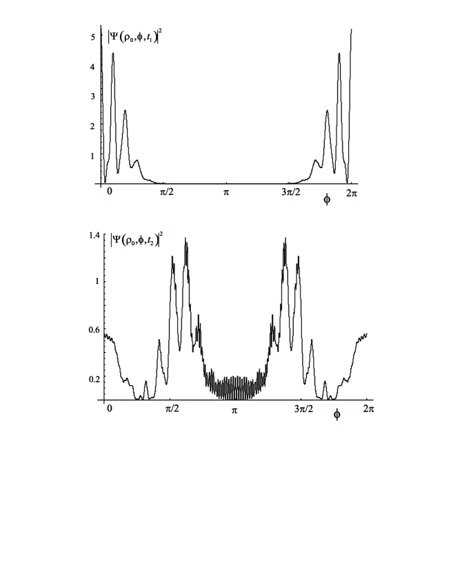
The result is displayed in Fig. 5, in the special case that . The average radius displays oscillations, which can be understood as arising from the outward motion due to the centrifugal potential, followed by reflection at the hard wall of the cylinder. The oscillations display collapse, followed by a revival. These may be viewed as arising from the initial dephasing of the contribution from the radial eigenfunctions with different values of , due to their energy difference. The revival of the oscillation can be understood from the discrete nature of the contributing energy eigenvalues, when the phase factors due to neighboring eigenenergies have built up a phase difference . Because of the conservation of angular momentum, the probability density near the origin remains zero. The interference between the counterrotating wave packets is illustrated in Fig. 6, for the ring at radius . Fig. 6a shows the short-time separation of the angular wave packets. Fig. 6b displays the interference that arises as soon as overlap occurs around between the clockwise and the anti-clockwise rotating packets. This demonstrates that the radial wave functions for different values of have sufficient overlap, so that the angular interference survives the effect of radial dispersion.
VII Conclusions
In this paper we describe the diffraction of an atomic wave by a circular optical lattice. Such a lattice can be formed by the superposition of two Laguerre-Gaussian beams with opposite helicity, which gives rise to a standing wave in the angular direction. Such a light field will split a single localized atom into clockwise and anticlockwise rotating components. If the system is in a trapping potential in the form of a ring or in a cylindrical box, these counterrotating components give rise to interference. We express the spatial pattern in the far diffraction field in terms of the Fourier transform of the near-field diffraction pattern. The periodic nature of the circular motion modifies this relation compared with the case of diffraction by a linear standing wave. The general conclusions are backed up by numerical calculations. Characteristic for the circular case is that the wave packets corresponding to opposite angular momentum will cross each other, even without applying light pulses to reverse their motion, as in more common interferometric schemes. The scheme is reasonably robust to changes in the radial confining potential.
ACKNOWLEDGMENTS
This work is part of the research program of the “Stichting voor Fundamenteel Onderzoek der Materie” (FOM).
REFERENCES
- [1] L. Allen, M. W. Beijersbergen, R. J. C. Spreeuw, and J. P. Woerdman, Phys. Rev. A 45, 8185 (1992).
- [2] S. S. R. Oemrawsingh, J. A. W. van Houwelingen, E. R. Eliel, J. P. Woerdman, E. J. K. Verstegen, J. G. Kloosterboer, G. W. t’ Hooft Appl. Opt., 43, 688 (2004).
- [3] S. J. van Enk and G. Nienhuis, J. Mod. Opt. 41, 963 (1994).
- [4] A. Muthukrishnan and C. R. Stroud Jr J. Opt. B: Quantum Semiclass. Opt. 4, S73 (2002).
- [5] M. E. J. Friese, J. Enger, H. Rubinsztein-Dunlop, and N. R. Heckenberg, Phys. Rev. A 54, 1593 (1996).
- [6] S. Kuppens, M. Rauner, M. Schiffer, K. Sengstock, W. Ertmer, F. E. van Dorsselaer, and G. Nienhuis, Phys. Rev. A 58, 3068 (1998).
- [7] E. M. Wright, J. Arlt, and K. Dholakia, Phys. Rev. A 63, 013608 (2001).
- [8] R. J. Cook and A. F. Bernhardt, Phys. Rev. A 18, 2533 (1978); A. Zh. Muradyan, Izv. Akad. Nauk Arm. SSR, Fiz. 10, 361 (1975); P. L. Gould, G. A. Ruff, and D. E. Pritchard, Phys. Rev. Lett. 56, 827 (1986).
- [9] P.R. Berman, ed., Atom Interferometry, (Academic Press, San Diego, 1997).
- [10] R.J. Cook and A. F. Bernhardt, Phys. Rev. A 18, 2533 (1978).
- [11] N. Tsukada, Phys. Rev. A 65, 063608 (2002); K. K. Das, G. J. Lapeyre, and E. M. Wright, Phys. Rev. A 65, 063603 (2002); Gh.-S. Paraoanu, Phys. Rev. A 67, 023607 (2003).