Minimal Informationally Complete Measurements for Pure States

Abstract

We consider measurements, described by a positive-operator-valued measure (POVM), whose outcome probabilities determine an arbitrary pure state of a $D$-dimensional quantum system. We call such a measurement a pure-state informationally complete (PS I-complete) POVM.  We show that a measurement with $2D-1$ outcomes cannot be PS I-complete, and then we construct a POVM with $2D$ outcomes that suffices, thus showing that a minimal PS I-complete POVM has $2D$ outcomes. We also consider PS I-complete POVMs that have only rank-one POVM elements and construct an example with $3D-2$ outcomes, which is a generalization of the tetrahedral measurement for a qubit. The question of the minimal number of elements in a rank-one PS I-complete POVM is left open.

I Introduction

An important technical requirement for developing coherent quantum technologies is the ability to assess how well one can prepare or create a particular quantum state. This assessment is carried out by making suitable measurements on a sequence of identically prepared quantum systems. The measurements are chosen so that the probabilities of the measurement outcomes suffice to determine the state; the probabilities are estimated from the outcome frequencies observed in the measurements. A set of measurements whose outcome probabilities are sufficient to determine an arbitrary quantum state is called informationally complete Prugovecki1977a ; Busch1989a . The process of determining the quantum state from the results of a sequence of these measurements is called quantum state tomography.

Given a set of measurements that are informationally complete, they can be amalgamated into a single generalized measurement, consisting of a coin flip to select a measurement from the set, followed by an application of that measurement. The statistics of such a generalized measurement are described by a positive-operator-valued measure (POVM) Peres1993a , which consists of positive operators $E^{\hskip 0.4ptc}$ that are labeled by an index $c$ that runs over the possible outcomes. These operators satisfy a completeness condition,

$$\sum_{c=1}^{n}E^{\hskip 0.4ptc}=\mathbb{I}\;.$$ (1)

The operators $E^{\hskip 0.4ptc}$, satisfying $0\leq E^{\hskip 0.4ptc}\leq\mathbb{I}$, are called POVM elements. The probability for outcome $c$, given system state $\rho$, is

$$p^{\hskip 1.0ptc}={\rm tr}(\rho E^{\hskip 0.4ptc})\;.$$ (2)

The completeness condition and the unit-trace normalization of $\rho$ guarantee that the probabilities are normalized to unity.

An informationally complete set of measurements can thus always be reformulated as a single informationally complete POVM (IC-POVM), i.e., a POVM having the property that the relations giving $p^{\hskip 1.0ptc}$ in terms of $\rho$ can be inverted to give $\rho$ in terms of the outcome probabilities. A normalized density operator $\rho$ is specified by $D^{2}-1$ real numbers, since an arbitrary Hermitian operator on a $D$-dimensional quantum system is specified by $D^{2}$ independent real numbers, and this number is reduced by one for a normalized density operator because it has unit trace. Since the relations (2) are linear, it is a simple matter of linear algebra to conclude that an IC-POVM must provide $D^{2}-1$ independent relations. This might lead one to think that an IC-POVM can get by with $D^{2}-1$ elements, but the normalization of the outcome probabilities means that one of the relations (2) is redundant, so an IC-POVM must have at least $D^{2}$ elements.

An equivalent, often more useful way of thinking is to disregard the normalization of the density operator. Then, like any Hermitian operator, $\rho$ is specified by $D^{2}$ real numbers, the additional number being ${\rm tr}(\rho)$. By virtue of the completeness condition, any POVM provides ${\rm tr}(\rho)$ as the sum of the (unnormalized) probabilities (2). This way of thinking bypasses the waffling about normalization conditions and goes directly to the point: an IC-POVM must provide $D^{2}$ linearly independent relations and thus must have at least $D^{2}$ POVM elements.

Informational completeness for arbitrary quantum states is thus equivalent to the ability to reconstruct any Hermitian operator $H$ from the operator inner products ${\rm tr}(HE^{\hskip 0.4ptc})$. This means that the problem of finding informationally complete POVMs is reduced to finding positive operators $F^{\hskip 0.4ptc}$ that span the vector space of Hermitian operators. If these operators don’t satisfy the completeness condition (1), one replaces them with the operators $E^{\hskip 0.4ptc}=G^{-1/2}F^{\hskip 0.4ptc}G^{-1/2}$, where $G=\sum_{c}F^{\hskip 0.4ptc}$ is trivially a nonsingular operator. The new operators are positive, satisfy the completeness condition, and are obviously informationally complete. Using this procedure, it is easy to construct minimal IC-POVMs, i.e., POVMs having $D^{2}$ elements, from sets of $D^{2}$ linearly independent, positive operators. Indeed, it is easy to construct minimal IC-POVMs for which all the POVM elements are rank-one, i.e., multiples of projectors onto pure states Caves2002b . Moreover, there is evidence, both analytical and numerical, that in all finite dimensions there are minimal, rank-one IC-POVMs, called symmetric, informationally complete POVMs (SIC-POVMs), for which the operator inner products of all pairs of POVM elements are the same Renes2004a . Recast as ensembles of states, SIC-POVMs have applications to quantum key distribution Renes2004b , and they have been shown Fuchs2004 to be the ensembles that are most quantum according to a measure of quantumness introduced by Fuchs and Sasaki Fuchs2003 .

In this paper we consider the pure-state version of informational completeness, i.e., reconstruction of an arbitrary pure state $\rho=|\psi\rangle\langle\psi|$ from the outcome probabilities

$$p^{\hskip 1.0ptc}=\langle\psi|E^{\hskip 0.4ptc}|\psi\rangle\;.$$ (3)

We formalize the notion of pure-state information completeness in the following definition.

Definition (PS I-completeness). A pure-state informationally complete (PS I-complete) POVM on a finite-dimensional quantum system is a POVM whose outcome probabilities are sufficient to determine any pure state (up to a global phase), except for a set of pure states that is dense only on a set of measure zero.

The intent of the last clause is to require the inversion to be unique for generic pure states. This clause says that any pure state outside a set of measure zero is surrounded by an open ball of states all of which are uniquely determined by the outcome probabilities.

Though some of the thinking and some of the mathematical techniques developed for IC-POVMs can be transferred to a study of PS I-complete POVMs, there is a critical difference, which makes PS I-completeness more difficult to analyze: the relation between the outcome probabilities and a density operator is linear, whereas the relation between outcome probabilities and pure states is quadratic. The problem of IC-POVMs thus lies squarely within linear algebra, whereas PS I-completeness must be tackled using other tools.

The first point to make about PS I-completeness arises from a simple counting argument. A pure state is specified by $D$ complex amplitudes, corresponding to $2D$ real numbers, but the number of independent real numbers is reduced to $2D-2$ by the normalization condition, $\langle\psi|\psi\rangle=1$, and by the fact that a pure state can be multiplied by a global phase without changing any of its predictions for probabilities. Because of the redundancy due to the normalization of the POVM probabilities, a PS I-complete POVM must contain at least one more element than the $2D-2$ real numbers to be determined. This suggests that a PS I-complete POVM might get by with only $2D-1$ elements. This argument can be profitably rephrased in terms of unnormalized pure states, which are specified by $2D-1$ real numbers, giving immediately that a PS I-complete POVM must have at least $2D-1$ elements. Unlike the similar counting argument for density operators, however, the counting argument for PS I-complete POVMs is only suggestive, because linear algebra can’t be applied to give rigorous conclusions. The counting argument leaves us only with a prejudice that the minimal number of elements in a PS I-complete POVM ought to be $2D-1$ or a little more.

The point of this paper is to provide some rigor. We establish that $2D$, not $2D-1$, is the minimal number of elements in a PS I-complete POVM.  To show this, we first prove that a POVM with fewer than $2D$ elements—in particular, one with $2D-1$ elements—cannot be PS I-complete (Sec. III), and we then construct an example of a PS I-complete POVM with $2D$ elements (Sec. IV).

Asher Peres considered a particular version of this problem in his classic 1993 quantum-mechanics textbook Peres1993a . He noted that the probabilities in two complementary bases should be sufficient to determine a pure state up to a finite set of ambiguities. If we let $\{|e_{j}\rangle,\;j=1,\ldots,D\}$, denote an orthonormal basis, the complementary basis consists of the vectors

$$|f_{k}\rangle={1\over\sqrt{D}}\sum_{j=1}^{D}|e_{j}\rangle\,e^{2\pi ijk/D}\;.$$ (4)

These complementary bases are discrete analogues of the position and momentum bases of a particle moving in one spatial dimension. A consequence of our work is that measurements in two complementary bases cannot be PS I-complete. To see this, notice that the amalgamated POVM for the two measurements has $2D$ POVM elements,

$$E^{\hskip 0.4ptc}=\cases{{1\over 2}|e_{c}\rangle\langle e_{c}|\;,&$c=1,\ldots,D$,\cr{1\over 2}|f_{c-D}\rangle\langle f_{c-D}|\;,&$c=D+1,\ldots,2D$.}$$ (5)

The factor of $1/2$ takes care of the coin flip that chooses with equal probability between measurements in the two bases. The probabilities associated with the last POVM element in each basis, $p^{D}={1\over 2}|\langle e_{D}|\psi\rangle|^{2}$ and $p^{2D}={1\over 2}|\langle f_{D}|\psi\rangle|^{2}$, provide no information because of the separate normalization of the measurements in the two bases. Without losing any information, we can combine these two POVM elements into a single element, ${1\over 2}(|e_{D}\rangle\langle e_{D}|+|f_{D}\rangle\langle f_{D}|)$, thus reducing the number of POVM elements to $2D-1$. Our proof in Sec. III shows this cannot be PS I-complete; attempts to find a pure state from the outcome probabilities must at least suffer from the finite ambiguities mentioned by Peres. Following Peres, we illustrate these ambiguities in two dimensions in Sec. II.

The problem considered by Peres is often called the Pauli problem, as it is the finite-dimensional version of a question posed by Pauli in a footnote to his quantum-mechanics article in Handbuch der Physik Pauli : can the wave function $\psi(x)$ of a particle be determined (up to a global phase) from the position and momentum probability distributions, $|\psi(x)|^{2}$ and $|\tilde{\psi}(p)|^{2}$? The answer to Pauli’s question is a definitive no: there are many wave functions not determined by their position and momentum distributions and thus said to be Pauli nonunique. Much work has been devoted to investigating Pauli nonunique states (see Refs. Busch1989a ; Weigert1992a ; Weigert1996a and references cited therein), but even now there does not seem to be a complete characterization of such wave functions. A simple example of a Pauli nonunique state is an eigenstate of parity, $\psi(x)=\pm\psi(-x)$ (and $\tilde{\psi}(p)=\pm\tilde{\psi}(-p)$), that is not time-reversal invariant, i.e., $\phi(x)=\psi^{*}(x)\neq e^{i\alpha}\psi(x)$; such a wave function satisfies $\tilde{\psi}^{*}(p)=\tilde{\phi}(-p)=\pm\tilde{\phi}(p)$, so $\psi(x)$ and $\phi(x)$, though distinct states, have the same position and momentum distributions. Discussion of work on Pauli nonunique states lies outside the scope of our paper, but we do note the interesting result of Corbett and Hurst Corbett1978a that Pauli nonunique wave functions are dense in the space of wave functions, a result that motivates the denseness restriction in our definition of PS I-completeness.

Previous work on PS I-completeness for finite-dimensional quantum systems Weigert1992a ; Amiet1999b ; Amiet1999c has considered the system to be a spin-$s$ particle ($D=2s+1$) and has focused mainly on reconstructing a pure state from the probabilities for spin components along several directions. The angular-momentum algebra and the rotation group play essential roles in these considerations. We review some of these results during the course of our discussion and point out how they are related to our work and, in particular, how they can be rephrased in terms of a single POVM.

Our paper is organized as follows. In Sec. II, we introduce informationally complete and PS I-complete POVMs in two dimensions and note that the two-dimensional case provides little guidance for generalizing PS I-completeness to higher dimensions. In Sec. III, we prove that the outcome probabilites of a POVM with $2D-1$ elements are insufficient to determine a general pure state in $D$ dimensions, leading to, at best, a two-state ambiguity. In Sec. IV, we construct a PS I-complete POVM with $2D$ elements, and in Sec. V, we turn to the question of rank-one PS I-complete POVMs and construct one with $3D-2$ POVM elements. Section VI gives a brief summary of open questions, while Sec. VII closes with a poetic description of one of these questions, dedicated to Asher Peres on the occasion of his 70th birthday.

II Informationally complete POVMs in two dimensions

We can gain some insight into IC-POVMs and PS I-complete POVMs by looking at the case of a two-dimensional quantum system (qubit), where the Bloch representation of states and operators permits us give a complete characterization of information completeness.

The Bloch representation of an arbitrary POVM element for a qubit is

$$E=a\mathbb{I}+b\bm{n}\cdot\bm{\sigma}\;,$$ (6)

where $\bm{n}$ is a unit vector in $\mathbb{R}^{3}$ and $a$ and $b$ are nonnegative real numbers satisfying $b\leq a$ and $b\leq 1-a$, to ensure that $E$ and $\mathbb{I}-E$ are positive operators. Rank-one POVM elements have $a=b$. A POVM is made up of $n$ such elements,

$$E^{\hskip 0.4ptc}=a^{c}\,\mathbb{I}+b^{c}\bm{n}^{c}\cdot\bm{\sigma}\;,\quad c=1,\ldots,n,$$ (7)

satisfying the completeness condition (1), which now becomes two conditions,

$$1 = \sum_{c}a^{c}\;,$$ (8)

$$0 = \sum_{c}b^{c}\bm{n}^{c}\;.$$ (9)

A POVM is informationally complete if and only if the POVM elements $E^{\hskip 0.4ptc}$ span the four-dimensional space of Hermitian operators. Translated to the Bloch representation, this says that a POVM is informationally complete if and only if the vectors $b^{c}\bm{n}^{c}$ span $\mathbb{R}^{3}$. A direct way to see this in the Bloch representation is to note that for an arbitrary density operator $\rho={1\over 2}(\mathbb{I}+\bm{P}\cdot\bm{\sigma})$, with polarization vector $\bm{P}$ ($|\bm{P}|\leq 1$), the outcome probabilities are given by

$$p^{\hskip 1.0ptc}=\mbox{tr}(\rho E^{\hskip 0.4ptc})=a^{c}+b^{c}\bm{n}^{c}\cdot\bm{P}\;;$$ (10)

to reconstruct an arbitrary polarization vector, the vectors $b^{c}\bm{n}^{c}$ must span $\mathbb{R}^{3}$.

The minimal number of elements in an IC-POVM is four; one sees this directly in the Bloch representation by noting that the vectors $b^{c}\bm{n}^{c}$ must span $\mathbb{R}^{3}$ and also satisfy the condition (9), implying that there must be at least four vectors. For a minimal IC-POVM, it is also easy to see from condition (9) that any three of the four vectors $b^{c}\bm{n}^{c}$ must be linearly independent and thus span $\mathbb{R}^{3}$ (and this means that none of the $b^{c}$ can be zero).

An example of a minimal, rank-one IC-POVM, which we make use of in Sec. V, is given by the tetrahedral measurement, which is specified by the four unit vectors

$$\bm{n}^{1} = \vphantom{{2\sqrt{2}\over 3}}(0,0,1)\;,$$

$$\bm{n}^{2} = \Biggl{(}{2\sqrt{2}\over 3},0,-{1\over 3}\Biggr{)}\;,$$

$$\bm{n}^{3} = \Biggl{(}-{\sqrt{2}\over 3},\sqrt{{2\over 3}},-{1\over 3}\Biggr{)}\;,$$

$$\bm{n}^{4} = \Biggl{(}-{\sqrt{2}\over 3},-\sqrt{{2\over 3}},-{1\over 3}\Biggr{)}\;,$$ (11)

with $a^{c}=b^{c}=1/4$, $c=1,2,3,4$. This POVM is also a SIC-POVM by virtue of the symmetric placement of the Bloch vectors, which connect the origin to the vertices of a tetrahedron whose apex is at the north pole of the Bloch sphere.

A PS I-complete measurement is one such that the outcome probabilities (10) determine uniquely a generic pure state $|\bm{m}\rangle\langle\bm{m}|={1\over 2}(\mathbb{I}+\bm{m}\cdot\bm{\sigma})$. It is immediately clear that to reconstruct an arbitrary unit vector $\bm{m}$, the vectors $b^{c}\bm{n}^{c}$ must span $\mathbb{R}^{3}$, so a PS I-complete measurement in two dimensions is always informationally complete for all states, pure or mixed. For this reason PS I-completeness for qubits provides little guidance for what happens in higher dimensions: in two dimensions, the $2D$ POVM elements required for PS I-completeness provide the $D^{2}$ elements necessary for informational completeness for all states, whereas in higher dimensions, there is a yawning gap between $2D$ and $D^{2}$.

It is worth stressing the way a three-element POVM fails to be PS I-complete. The condition (9) implies that the three vectors $b^{c}\bm{n}^{c}$ are linearly dependent and thus span at most a plane. The outcome probabilities (10) provide no information about the component of $\bm{m}$ orthogonal to the plane. When the vectors $b^{c}\bm{n}^{c}$ do span a plane, the outcome probabilities determine the projection of $\bm{m}$ onto this plane, which specifies everything about $\bm{m}$ except the sign of the component orthogonal to the plane. This two-fold ambiguity is the source of the POVM’s incompleteness for pure states.

A symmetric example of a three-outcome, rank-one measurement is the trine measurement on a qubit Peres1992a , given by the unit vectors

$$\bm{n}^{1} = \vphantom{{1\over 2}}(1,0,0)\;,$$

$$\bm{n}^{2} = \Biggl{(}-\frac{1}{2},\frac{\sqrt{3}}{2},0\Biggr{)}\;,$$

$$\bm{n}^{3} = \Biggl{(}-\frac{1}{2},-\frac{\sqrt{3}}{2},0\Biggr{)}\;,$$ (12)

with $a^{c}=b^{c}=1/3$, $c=1,2,3$. These vectors point from the origin to the vertices of an equilateral triangle lying in the equatorial plane of the Bloch sphere. The outcome probabilities for the trine determine the equatorial component of the Bloch vector for a pure state, but can’t resolve whether the Bloch vector is in the northern hemisphere or the southern hemisphere, thus leaving a two-state ambiguity.

III Necessity of $2D$ or more outcomes

In this section we show that the outcome probabilities of a POVM with $2D-1$ outcomes are insufficient to determine a generic pure state. In particular, we prove the following theorem.

Theorem. The outcome probabilities $p^{\hskip 1.0ptc}=\langle\psi|E^{\hskip 0.4ptc}|\psi\rangle$ of a POVM with $2D-1$ measurement outcomes are insufficient to determine a generic pure state $|\psi\rangle$ in $D$ dimensions.

We prove the theorem by showing that any allowed distribution of outcome probabilities, except a set of distributions of measure zero, is consistent with at least two possible pure states. The proof occupies the remainder of this section.

We begin by picking a particular POVM element, say $E^{1}$, and writing it in its orthonormal eigenbasis $\{|j\rangle,\;j=0,\ldots,D-1\}$:

$$E^{1}=\sum_{j=0}^{D-1}\lambda_{j}|j\rangle\;.$$ (13)

We order the eigenvalues from smallest to largest, i.e., $0\leq\lambda_{0}\leq\lambda_{1}\leq\ldots\leq\lambda_{D-1}$. We can assume that $\lambda_{D-1}>\lambda_{0}$, because otherwise $E^{1}$ would be a multiple of the identity operator and would provide no useful information beyond that always contained in the normalization constraint. Any pure state can be expanded in this eigenbasis as

$$|\psi\rangle=r_{0}|0\rangle+\sum_{j=1}^{D-1}c_{j}|j\rangle\;.$$ (14)

We use the global phase freedom to make $r_{0}$ real, but we do not require $|\psi\rangle$ to be normalized. Instead we consider the norm to be an extra parameter of the state, which is determined by the sum of the (unnormalized) outcome probabilities (3),

$$\sum_{c=1}^{2D-1}p^{\hskip 1.0ptc}=\langle\psi|\psi\rangle\equiv R^{2}\;,$$ (15)

by virtue of the completeness condition (1) for our POVM.

The amplitudes $c_{j}$ are arbitrary complex numbers, which we now write in terms of their real and imaginary parts, i.e., $c_{j}=x_{j}+iy_{j}$. The variables necessary to define the state are now the $2D-1$ real co-ordinates $r_{0}$, $x_{1},\ldots,x_{2D-1},y_{1},\ldots,y_{2D-1}$, each of which is free to take on any real value. We find it convenient to put all these co-ordinates into a single real vector $\bm{\xi}\in\mathbb{R}^{2D-1}$, whose components are

$$\xi_{0} = r_{0}\;,$$

$$\xi_{j} = x_{j}\quad\text{and}\quad\xi_{j+D-1}=y_{j}\;,\quad j=1,\ldots,D-1.$$ (16)

Notice that an inversion through the origin, i.e., $\bm{\xi}\rightarrow-\bm{\xi}$, produces a global sign change in $|\psi\rangle$. When $r_{0}=\xi_{0}\neq 0$, we could remove the global phase freedom entirely by making $\xi_{0}$ positive, but we choose to retain this two-fold ambiguity so that the space we are dealing with is the entirety of $\mathbb{R}^{2D-1}$.

Each of the $2D-1$ outcome probabilities can now be written as a quadratic form

$$p^{\hskip 1.0ptc}=\langle\psi|E^{\hskip 0.4ptc}|\psi\rangle=\sum_{r,s}\xi_{r}M^{c}_{rs}\,\xi_{s}\;,$$ (17)

where the quantities $M^{c}_{rs}$ are the matrix elements of a real, symmetric, positive (semi-definite) matrix ${\sf M}^{c}$. A surface of constant $p^{\hskip 1.0ptc}>0$ is a $2(D-1)$-dimensional (possibly degenerate) hyperellipsoid ${\cal E}_{p^{\hskip 1.0ptc}}$, which extends to $\pm\infty$ in a number of dimensions given by $2D-1-{\rm rank}({\sf M}^{c})$ and has a hyperellipsoidal cross-section in the remaining dimensions, numbering ${\rm rank}({\sf M}^{c})$. Notice that by construction the first outcome probability has a diagonal matrix ${\sf M}^{1}$,

$$p^{1}=\lambda_{0}r_{0}^{2}+\sum_{j=1}^{D-1}\lambda_{j}|c_{j}|^{2}=\lambda_{0}\xi_{0}^{2}+\sum_{j=1}^{D-1}\lambda_{j}(\xi_{j}^{2}+\xi_{j+D-1}^{2})\;,$$ (18)

and is thus a hyperellipsoid aligned with the co-ordinate axes.

We now replace two of the outcome probabilities by equivalent constraints. First we replace the last outcome probability ($c=2D-1$) by the normalization condition (15),

$$R^{2}=\langle\psi|\psi\rangle=\sum_{r=0}^{2D-2}\xi_{r}^{2}\;,$$ (19)

something we can do because $p^{2D-1}=R^{2}-\sum_{c=1}^{2D-2}p^{\hskip 1.0ptc}$. A surface of constant norm $R^{2}$ is, of course, a sphere ${\cal S}_{R}$ of radius $R$ in $\mathbb{R}^{2D-1}$. Each physical state $|\psi\rangle$ with $\xi_{0}\neq 0$ is represented twice on this sphere of radius $R$, once in the northern hemisphere ($\xi_{0}>0$) and again, with its sign reversed, at the antipode in the southern hemisphere ($\xi_{0}<0$). States on the equator ($\xi_{0}=0$) retain the full global phase freedom.

The second modification is to replace the first outcome probability (18) with an equivalent constraint in which $\xi_{0}$ does not appear:

$$p^{1}-\lambda_{0}R^{2}=\sum_{j=1}^{D-1}(\lambda_{j}-\lambda_{0})(\xi_{j}^{2}+\xi_{j+D-1}^{2})\equiv P\geq 0\;.$$ (20)

That $P\geq 0$ follows because $\lambda_{0}$ is the smallest eigenvalue. Moreover, we are guaranteed that $P$ is not always zero because $\lambda_{D-1}>\lambda_{0}$. All this means that a surface of constant $P>0$ is a hyperellipsoid ${\cal E}_{P}$, aligned with the $\xi_{r}$ axes, which runs off to $\pm\infty$ along the $\xi_{0}$ axis (and perhaps other axes) and which has an ellipsoidal boundary in one or more co-ordinates $\xi_{r}$.

Now consider a particular set of values for $R^{2}$, $p^{2D-2},\ldots,p^{2}$, and $P$, and imagine applying the constraints imposed by these $2D-1$ measured values in the order listed. The first step in the process yields the submanifold ${\cal I}_{1}\equiv{\cal E}_{R^{2}}={\cal S}_{R}$. The set ${\cal I}\hskip 0.3pt_{m}$ obtained after $m$ steps is the intersection of ${\cal I}\hskip 0.3pt_{m-1}$ with the hyperellipsoidal submanifold ${\cal E}_{p^{2D-m}}$,

$${\cal I}\hskip 0.3pt_{m}={\cal I}\hskip 0.3pt_{m-1}\cap{\cal E}_{p^{2D-m}}\;.$$

The last step intersects ${\cal I}\hskip 0.3pt_{2D-2}$ with ${\cal E}_{P}$ to yield the set ${\cal I}\hskip 0.3pt_{2D-1}={\cal I}\hskip 0.3pt_{2D-2}\cap{\cal E}_{P}$. We note that for all $m$, ${\cal I}\hskip 0.3pt_{m}$ is a compact set because the process starts with the sphere ${\cal S}_{R}$, which is itself compact. For PS I-completeness the final set ${\cal I}\hskip 0.3pt_{2D-1}$ must consist generically of just the two antipodal points representing a particular pure state.

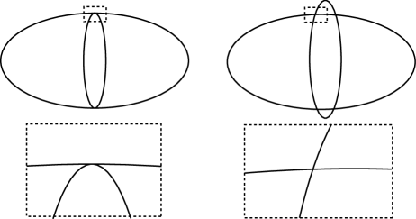
Figure 1: Transversal and nontransversal intersections. The two ellipses shown in each subfigure are submanifolds of $\mathbb{R}^{2}$. a) shows a nontransversal intersection of two ellipses, and b) is a close-up of one of the intersection points. The intersection in b) is nontransversal because the tangent vectors at the point shown are the same; they therefore span only a one-dimensional subspace of $\mathbb{R}^{2}$. c) shows a slight perturbation of a), and by looking at the close-up of the intersection in d), we see that the intersection is now transversal. This is because at all points of intersection, the tangent vectors of the two submanifolds span $\mathbb{R}^{2}$.

Having set up the entire problem, we now need a bit of differential geometry about the intersection of submanifolds. Given a manifold $R$ of dimension $d_{R}$, two submanifolds, $M$ and $N$, of dimensions $d_{M}$ and $d_{N}$, intersect transversally if at each point of intersection ${\cal P}$, the vectors in the tangent spaces to $M$ and $N$, $T_{M}({\cal P})$ and $T_{N}({\cal P})$, span the entire tangent space to $R$ at ${\cal P}$ (see Fig. 1). A transversal intersection $M\cap N$ is a submanifold of dimension $d_{M\cap N}=d_{M}+d_{N}-d_{R}$, since this relation holds for the dimensions of the tangent spaces at each point of intersection. A fundamental theorem of differential geometry, called Sard’s theorem sard , asserts that if two submanifolds with a nonempty intersection intersect nontransversally, they can be perturbed slightly to intersect transversally. Figure 1 illustrates the difference between transversal and nontransversal intersections and how a perturbation of a nontransversal intersection yields a transversal intersection.

We now apply these ideas to our situation. Notice that if the successive intersections in our sequence are transversal, then each intersection produces a new submanifold with dimension decreased by one, $d_{{\cal I}\hskip 0.3pt_{m}}=d_{{\cal I}\hskip 0.3pt_{m-1}}+(2D-2)-(2D-1)=d_{{\cal I}\hskip 0.3pt_{m-1}}-1$, so the dimension of $I_{m}$ is $2D-1-m$. We now argue that if the measurement is to be PS I-complete, a sequence of such transversal intersections must occur generically, i.e., for all outcome probabilities $p^{c}$ except for a set of measure zero.

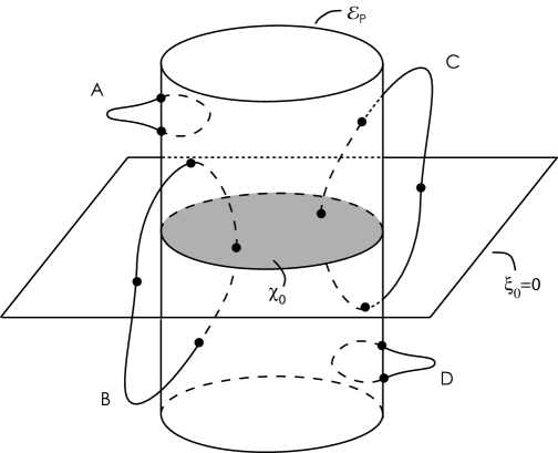
Figure 2: The cylinder is the hyperellipsoidal submanifold ${\cal E}_{P}$ with many dimensions suppressed. Recall that ${\cal E}_{P}$ extends to infinity, though it is drawn as finite here. The union of the closed curves $A$, $B$, $C$, and $D$ is the submanifold ${\cal I}\hskip 0.3pt_{2D-2}$. The convention for dashed and dotted lines is that lines that are behind one layer of the cylinder are dashed, and lines that are behind two layers are dotted. The points where ${\cal I}\hskip 0.3pt_{2D-2}$ intersects ${\cal E}_{P}$ (denoted as black dots) are the (zero-dimensional) submanifold ${\cal I}\hskip 0.3pt_{2D-1}$. Notice that the entire diagram is invariant under inversion through the origin. The shaded disk ${\cal X}_{0}$, which is the part of the $\xi_{0}=0$ hyperplane that is in or on the interior of the ${\cal E}_{P}$ submanifold, also has inversion-symmetric points of intersection with ${\cal I}\hskip 0.3pt_{2D-2}$. The part of ${\cal E}_{P}$ with $\xi_{0}>0$, denoted in the text as ${\cal E}^{(+)}_{P}$, has multiple intersections with ${\cal I}\hskip 0.3pt_{2D-2}$, implying that Eqs. (17) cannot be inverted to reconstruct a unique pure state $|\psi\rangle$.

Suppose instead that the intersections are transversal up to the $m$th step, at which step ${\cal I}\hskip 0.3pt_{m-1}$ and ${\cal E}_{p^{2D-m}}$ intersect nontransversally. There are two ways this could happen. First, it could be that part or all of ${\cal I}\hskip 0.3pt_{m-1}$ lies in ${\cal E}_{p^{2D-m}}$, so that part or all of the intersection fails to have dimension reduced by one. If this situation were generic, it would mean that the final intersection would be greater than zero-dimensional, thus not specifying points, so the POVM could not be PS I-complete. Second, it could be that part or all of the intersection has dimensionality reduced by more than one, as in the case of two ellipsoids touching at tangent points. This is the situation depicted in Figure 1a) if the ellipses were replaced with surfaces of revolution about the vertical axis in the diagram. If this situation were generic, it would imply a relation between the $m$ remaining values, $p^{2D-m},\ldots,P$, and the previous values, $R^{2},\ldots,p^{2D-m+1}$; since an arbitrary state is not subject to such a restriction, the POVM could not be PS I-complete. We conclude that if a measurement is to be PS I-complete, a transversal intersection at every step in our process is generically necessary. In accordance with Sard’s theorem, a nontransversal intersection at any step could be removed by slightly perturbing the values of our constraints.

Now consider the final step in our process. As we have just argued, if the POVM is to be PS I-complete, this step generically involves the transversal intersection of a compact, one-dimensional submanifold, ${\cal I}\hskip 0.3pt_{2D-2}$, with the hyperellipsoid ${\cal E}_{P}$, which is defined by Eq. (20) (with $P>0$ generically), and the result of this final intersection is a set of points, ${\cal I}\hskip 0.3pt_{2D-1}$. The submanifold ${\cal I}\hskip 0.3pt_{2D-2}$, being compact and one-dimensional, is a set of closed curves that do not intersect one another or themselves. Moreover, the hyperellipsoid ${\cal E}_{P}$ is closed and orientable, thus splitting $\mathbb{R}^{2D-1}$ into an inside and an outside. A closed curve intersecting such a surface transversally must intersect it an even number of times, since any entrance from the outside must be paired with an exit. Thus we can conclude that ${\cal I}\hskip 0.3pt_{2D-1}$ consists generically of an even number of points.

We need, of course, a stronger result than this because the inversion symmetry, $\bm{\xi}\rightarrow-\bm{\xi}$, already implies that the points in ${\cal I}\hskip 0.3pt_{2D-1}$ come in pairs. What we need to show is that ${\cal I}\hskip 0.3pt_{2D-1}$ contains at least two points with $\xi_{0}>0$, but we can get this by a simple extension of the above reasoning, which is illustrated in Fig. 2. Let ${\cal X}_{0}$ be the part of the hyperplane $\xi_{0}=0$ that lies inside or on ${\cal E}_{P}$. The inversion symmetry guarantees that the points in the intersection of ${\cal I}\hskip 0.3pt_{2D-2}$ with ${\cal X}_{0}$ come in pairs, $\bm{\xi}$ and $-\bm{\xi}$. The points in a pair are distinct, because an intersection at $\bm{\xi}=0$ is forbidden by the normalization constraint.

Now consider the union of the $\xi_{0}>0$ part of ${\cal E}_{P}$, which we denote as ${\cal E}_{P}^{(+)}$, and ${\cal X}_{0}$. Since this union is closed and orientable, we can conclude, just as we did above for ${\cal E}_{P}$, that the closed curves in ${\cal I}\hskip 0.3pt_{2D-2}$ intersect it an even number of times. Since we have just established that ${\cal I}\hskip 0.3pt_{2D-2}$ intersects ${\cal X}_{0}$ an even number of times, we find that ${\cal I}\hskip 0.3pt_{2D-2}$ intersects ${\cal E}_{P}^{(+)}$ an even number of times. This means that the final set, ${\cal I}\hskip 0.3pt_{2D-1}$, generically has an even number of points with $\xi_{0}>0$, corresponding to distinct pure states consistent with the outcome probabilities. This completes the proof of Theorem 1, because this generic ambiguity, at least two-fold, shows that a POVM with $2D-1$ elements cannot be PS I-complete.

IV Sufficiency of $2D$ outcomes

In this section we construct an explicit example of a PS I-complete POVM with $2D$ outcomes, thus showing the sufficiency of this number of outcomes for PS I-completeness. Combined with the result of the preceding section, this shows that a minimal PS I-complete POVM has $2D$ elements.

Letting $\{|j\rangle,\;j=0,\ldots,D-1\}$ denote an orthonormal basis for a $D$-dimensional quantum system, we define the operators

$$X_{jk} \equiv |j\rangle\langle k|+|k\rangle\langle j|\;,$$

$$Y_{jk} \equiv -i|j\rangle\langle k|+i|k\rangle\langle j|\;,$$ (21)

$$Z_{jk} \equiv |j\rangle\langle j|-|k\rangle\langle k|\;.$$

These operators can be thought of as the Pauli operators in the subspace spanned by $|j\rangle$ and $|k\rangle$. In this section we only need the $0j$ versions of these operators, but we use others in Sec. V.

We now consider a POVM consisting of the following positive operators:

$$a|0\rangle\langle 0|\;,$$

$$b(\mathbb{I}+X_{0j})\quad\text{and}\quad b(\mathbb{I}+Y_{0j})\;,\quad\mbox{$j=1,\ldots,D-1$,}$$ (22)

$$T\;.$$

Here $a$ and $b$ are positive numbers, and $T$ is a “throw-away” POVM element that must be included to satisfy the completeness condition (1). We can always make $T$ a positive operator by choosing $a$ and $b$ small enough. Notice that this POVM has $2D$ elements, as promised. We now demonstrate that this POVM is PS I-complete.

We let

$$|\psi\rangle=\sum_{j=0}^{D-1}c_{j}|j\rangle$$ (23)

be an arbitrary normalized pure state, expanded in the basis $\{|j\rangle\}$. We remove the global phase freedom by choosing $c_{0}=r_{0}$ to be real and nonnegative, and we write $c_{j}=x_{j}+iy_{j}$ for the remaining amplitudes.

The first outcome probability for the POVM (22) is

$$p^{0}=a|\langle 0|\psi\rangle|^{2}=ar_{0}^{2}\;,$$ (24)

from which we get the (positive) amplitude of the state $|0\rangle$,

$$r_{0}=\sqrt{\frac{p^{0}}{a}}\;.$$ (25)

The remaining outcome probabilities (except for the throw-away outcome) are

$$p^{\hskip 0.6ptx,j} = b\langle\psi|(\mathbb{I}+X_{0j})|\psi\rangle=b(1+2r_{0}x_{j})\;,$$

$$p^{\hskip 0.8pty,j} = b\langle\psi|(\mathbb{I}+Y_{0j})|\psi\rangle=b(1+2r_{0}y_{j})\;,$$ (26)

for $j=1,\ldots,D-1$. Except for states with $r_{0}=0$ (a set of measure zero), these, too, can be immediately inverted to give the remaining amplitudes,

$$x_{j} = \frac{p^{\hskip 0.6ptx,j}-b}{2br_{0}}\;,$$ (27)

$$y_{j} = \frac{p^{\hskip 0.8pty,j}-b}{2br_{0}}\;.$$ (28)

This completes the (trivial) demonstration that the POVM (22) is PS I-complete.

The inversion procedure fails on the $(D-1)$-dimensional subspace orthogonal to $|0\rangle$, where $r_{0}=0$. There is a simple way to handle this failure in a tomographic procedure, i.e., in a sequence of measurements of this POVM, made on many identical copies of the same system, with the outcome probabilities estimated from the outcome frequencies. All one has to do is to precede the tomographic procedure with a single premeasurement in the basis $\{|j\rangle\}$. Whatever the outcome of this premeasurement, that outcome has nonzero probability, so we can choose it to be the state $|0\rangle$.

Notice that after determining $r_{0}$, the reconstruction of the remaining amplitudes $c_{j}$ is reduced to solving linear equations. This transformation of a fundamentally quadratic inversion into a linear one is the reason it is so easy to show that the POVM (22) is PS I-complete. The key to this transformation is that the probabilities (26) have no terms that are quadratic in the amplitudes $c_{j}$. This, in turn, is a consequence of having the unit operator in the “middle” POVM elements, $b(\mathbb{I}+X_{0j})$ and $b(\mathbb{I}+Y_{0j})$, since for normalized states, these unit operators always put a 1 into the corresponding outcome probabilities. We can’t just leave the unit operator out, because we have to put something there to make the middle POVM elements positive. Suppose, for example, that we tried to make the middle POVM elements rank one by changing them to $b(P_{0j}+X_{0j})$ and $b(P_{0j}+Y_{0j})$, where $P_{0j}=|0\rangle\langle 0|+|j\rangle\langle j|$ is the projection operator onto the subspace spanned by $|0\rangle$ and $|j\rangle$. Then the probabilities (26) become $p^{\hskip 0.6ptx,j}=b(r_{0}^{2}+x_{j}^{2}+y_{j}^{2}+2r_{0}x_{j})$ and $p^{\hskip 0.8pty,j}=b(r_{0}^{2}+x_{j}^{2}+y_{j}^{2}+2r_{0}y_{j})$. The quadratic term $x_{j}^{2}+y_{j}^{2}$ introduces a generic two-fold ambiguity into the determination of each of the amplitudes $c_{j}$, which makes the POVM not PS I-complete.

We should stress that the role of the POVM (22) is solely to demonstrate that $2D$ outcomes are sufficient for PS I-completeness, because the presence of the unit operator in the middle POVM elements makes this POVM a poor candidate indeed for an actual tomographic procedure. The unit operators mean that the middle outcomes all have nearly the same probability, with only a weak dependence on the amplitudes $c_{j}$. It is from this weak dependence that one must extract the amplitudes, and this makes a tomographic procedure based on this POVM very inefficient.

Weigert Weigert1992a has described a quite different way of making a PS I-complete measurement, which we can manipulate to produce a single PS I-complete POVM with $2D$ outcomes. Considering the system to be a spin-$s$ particle ($D=2s+1$), Weigert first shows that the probabilities for two spin components, $\bm{S}\cdot\bm{n}$ and $\bm{S}\cdot\bm{n}^{\prime}$, along infinitesimally different directions, are sufficient to determine a generic pure state up to $2^{2s}=2^{D-1}$ ambiguities. He then shows that the ambiguities can be resolved by knowing just the expectation value of the spin component $\bm{S}\cdot\bm{e}$ along the direction $\bm{e}$ orthogonal to $\bm{n}$ and $\bm{n}^{\prime}$.

To describe this scheme, let $|\bm{n},m\rangle$ denote the eigenvector of $\bm{S}\cdot\bm{n}$ with eigenvalue $m$. Notice that

$$F\equiv{1\over 2s}(\bm{S}\cdot\bm{e}+s\mathbb{I})={1\over 2s}\sum_{m=-s}^{s}(s+m)|\bm{e},m\rangle\langle\bm{e},m|$$ (29)

is a potential POVM element whose expectation value contains the same information as the expectation value of $\bm{S}\cdot\bm{e}$. Weigert describes getting the expectation value of $\bm{S}\cdot\bm{e}$ in the standard way from measurements of that spin component, but we can get the same information directly by including $F$ in a POVM.  Furthermore, since the measurements of $\bm{S}\cdot\bm{n}$ and $\bm{S}\cdot\bm{n}^{\prime}$ are separately normalized, we can amalgamate two projectors, one from each measurement, into a single POVM element without losing any information. If we put all this together, Weigert’s work shows that a generic pure state is determined by the expectation values of the operators

$$|\bm{n},m\rangle\langle\bm{n},m|\;,\quad m=-s+1,\ldots,s,$$

$$|\bm{n}^{\prime},m\rangle\langle\bm{n}^{\prime},m|\;,\quad m=-s+1,\ldots,s,$$

$$|\bm{n},-s\rangle\langle\bm{n},-s|+|\bm{n}^{\prime},-s\rangle\langle\bm{n}^{\prime},-s|\;,$$

$$F\;.$$ (30)

This list contains $2D$ POVM elements, whose expectation values are PS I-complete, but the list does not constitute a POVM because the elements don’t sum to $\mathbb{I}$. To turn the list into a POVM, we use a trick mentioned in the Introduction in the context of IC-POVMs. Suppose we have a set of positive operators, $\{F^{\hskip 0.4ptc}\}$, which are PS I-complete in that their expectation values are sufficient to reconstruct a generic unnormalized vector $|\psi\rangle$ up to a global phase. First form the operator $G=\sum_{c}F^{\hskip 0.4ptc}$. This operator is invertible, for if it weren’t, there would be a vector $|e\rangle$ such that $\langle e|G|e\rangle=0$, which would imply that $F^{\hskip 0.4ptc}|e\rangle=0$ for all values of $c\,$; this would mean that the expectation values of the operators $F^{\hskip 0.4ptc}$ provide no information about the amplitude $\langle e|\psi\rangle$, so the operators would not be informationally complete. Now define new operators $E^{\hskip 0.4ptc}=G^{-1/2}F^{\hskip 0.4ptc}G^{-1/2}$. These operators are positive and sum to $\mathbb{I}$, so they make up a POVM; moreover, they are obviously PS I-complete. It is also worth noting that if $F^{\hskip 0.4ptc}$ is rank-one, so is $E^{\hskip 0.4ptc}$.

Although it is easy to calculate $G$ for the list (30), it is not very enlightening to calculate the POVM elements. We simply note that the trick can be applied to the list (30), thereby turning Weigert’s PS I-complete measurements into a minimal PS I-complete POVM—and, moreover, one with $2D-2$ rank-one POVM elements. The price of this transformation is that the measurement no longer corresponds to just measuring a few spin components.

One might be tempted to apply this trick to the POVM elements (22), without the throw-away $T$, since the probability for outcome $T$ never appears in the inversion procedure. We know this can’t work, however, because the result would be a PS I-complete POVM with $2D-1$ elements, contradicting the results of Sec. III. The reason it doesn’t work is that the inversion procedure assumes normalized pure states, and the trick only works if the inversion works for normalized and unnormalized states. For unnormalized states, the throw-away can’t be discarded because it is required to fix the normalization.

V Rank-one PS I-complete measurement with $3D-2$ outcomes

In this section we consider PS I-complete POVMs whose POVM elements are all of rank one, i.e., multiples of one-dimensional projectors. We don’t know the minimal number of elements in a rank-one PS I-complete POVM. We suspect it is close to or even equal to $2D$—the reworked Weigert measurement discussed in Sec. IV has $2D$ elements, with just two not of rank one—but the best we can do for the present is $3D-2$ elements, an example of which we present now.

The setting here is the same as in Sec. IV, with states and operators defined as in Eqs. (23) and (21), except that we now allow the states $|\psi\rangle$ to be unnormalized. Consider the following four states in the subspace spanned by $|j\rangle$ and $|k\rangle$,

$$|\psi_{jk;0}\rangle = |j\rangle\;,$$

$$|\psi_{jk;1}\rangle = \cos(\theta/2)|j\rangle+\sin(\theta/2)|k\rangle\;,$$

$$|\psi_{jk;2}\rangle = \cos(\theta/2)|j\rangle+e^{2\pi i/3}\sin(\theta/2)|k\rangle\;,$$

$$|\psi_{jk;3}\rangle = \cos(\theta/2)|j\rangle+e^{-2\pi i/3}\sin(\theta/2)|k\rangle\;,$$ (31)

where we assume $0<\theta<\pi$. Notice that we can write

$$|\psi_{jk;\alpha}\rangle=\cos(\theta/2)|j\rangle+e^{2\pi i(\alpha-1)/3}\sin(\theta/2)|k\rangle\;,\quad\alpha=1,2,3.$$ (32)

The corresponding one-dimensional projection operators are given by

$$|\psi_{jk;0}\rangle\langle\psi_{jk;0}| = {1\over 2}\left(P_{jk}+Z_{jk}\right)\;,$$

$$|\psi_{jk;1}\rangle\langle\psi_{jk;1}| = {1\over 2}\left(P_{jk}+X_{jk}\sin\theta+Z_{jk}\cos\theta\right)\;,$$

$$|\psi_{jk;2}\rangle\langle\psi_{jk;2}| = {1\over 2}\left(P_{jk}-X_{jk}{1\over 2}\sin\theta+Y_{jk}\sqrt{{3\over 2}}\sin\theta+Z_{jk}\cos\theta\right)\;,$$

$$|\psi_{jk;3}\rangle\langle\psi_{jk;3}| = {1\over 2}\left(P_{jk}-X_{jk}{1\over 2}\sin\theta-Y_{jk}\sqrt{{3\over 2}}\sin\theta+Z_{jk}\cos\theta\right)\;.$$ (33)

When $\cos\theta=-1/3$, these are the four tetrahedral states in the two-dimensional subspace spanned by $|j\rangle$ and $|k\rangle$; in this subspace, they are specified by the Bloch vectors (11). Notice that

$$\sum_{\alpha=1}^{3}|\psi_{jk;\alpha}\rangle\langle\psi_{jk;\alpha}|={3\over 2}(P_{jk}+Z_{jk}\cos\theta)=3\Bigl{(}\cos^{2}(\theta/2)|j\rangle\langle j|+\sin^{2}(\theta/2)|k\rangle\langle k|\Bigr{)}\;.$$ (34)

We now consider the following POVM elements, numbering $3D-2$,

$$a|0\rangle\langle 0|\;,$$

$$b|\psi_{j-1,j\,;\,\alpha}\rangle\langle\psi_{j-1,j\,;\,\alpha}|\;,\quad j=1,\ldots,D-1,\quad\alpha=1,2,3,$$ (35)

where we assume $a,b>0$. The first thing to show is that these POVM elements are sufficient to reconstruct a generic unnormalized pure state $|\psi\rangle$. We begin by determining $c_{0}=r_{0}>0$ from the probability for the first POVM element, $a|\langle 0|\psi\rangle|^{2}=ar_{0}^{2}$. As we work through the remaining amplitudes, suppose that we have determined $c_{0},\ldots,c_{j-1}$ and are now trying to get $c_{j}$ from the three POVM probabilities

$$b\bigl{|}\langle\psi_{j-1,j\,;\,\alpha}|\psi\rangle\bigr{|}^{2}=b\bigl{|}\cos(\theta/2)c_{j-1}+e^{-2\pi i(\alpha-1)/3}\sin(\theta/2)c_{j}\bigr{|}^{2}\;,\quad\alpha=1,2,3.$$ (36)

Writing these three probabilities out, it becomes clear that they determine $c_{j}$, provided $c_{j-1}\neq 0$. The only hitch in this method is that we get stuck if any $c_{j}$ except the last is zero, so we have a set of $D-1$ $(D-1)$-dimensional subspaces where the method fails. This failure set is a set of measure zero, however, so the procedure succeeds in reconstructing a generic pure state.

We now use the trick that we applied to Weigert’s measurement in Sec. IV. We form the sum of the operators in Eq. (35),

$$G = a|0\rangle\langle 0|+\sum_{j=1}^{D-1}\sum_{\alpha=1}^{3}b|\psi_{j-1,j\,;\,\alpha}\rangle\langle\psi_{j-1,j\,;\,\alpha}|$$ (37)

$$= \bigl{(}a+3b\cos^{2}(\theta/2)\bigr{)}|0\rangle\langle 0|+3b\sum_{j=1}^{D-2}|j\rangle\langle j|+3b\sin^{2}(\theta/2)|D-1\rangle\langle D-1|\;,$$

where we use the sum (34). Choosing $b=1/3$ and $a=\sin^{2}(\theta/2)$, we get

$$G=\mathbb{I}-\cos^{2}(\theta/2)|D-1\rangle\langle D-1|\;.$$ (38)

The trick introduced in Sec. IV now tells us that the following POVM elements make up a POVM that is PS I-complete:

$$\sin^{2}(\theta/2)G^{-1/2}|0\rangle\langle 0|G^{-1/2}=\sin^{2}(\theta/2)|0\rangle\langle 0|\;,$$

$${1\over 3}G^{-1/2}|\psi_{j-1,j\,;\,\alpha}\rangle\langle\psi_{j-1,j\,;\,\alpha}|G^{-1/2}={1\over 3}|\psi_{j-1,j\,;\,\alpha}\rangle\langle\psi_{j-1,j\,;\,\alpha}|\;,\quad j=1,\ldots,D-2,\quad\alpha=1,2,3,$$

$${1\over 3}G^{-1/2}|\psi_{D-2,D-1;\alpha}\rangle\langle\psi_{D-2,D-1;\alpha}|G^{-1/2}\;,\quad\alpha=1,2,3.$$ (39)

Here

$$G^{-1/2}|\psi_{D-2,D-1;\alpha}\rangle=\cos(\theta/2)|D-2\rangle+e^{2\pi i(\alpha-1)/3}|D-1\rangle\;,\quad\alpha=1,2,3.$$ (40)

It is easy to see directly, without appealing to the general validity of our trick, that these particular elements make up a rank-one POVM that is PS I-complete.

Notice that $D=2$ is a special case, because the sum in the second form of Eq. (37) is missing. By making the tetrahedral choice of angle with $a=b=1/2$, we get the four-element tetrahedral POVM of Eq. (11). Thus the POVM (39) can be considered as a sort of generalization of the tetrahedral measurement.

Amiet and Weigert Amiet1999b have formulated a PS I-complete measurement procedure for a spin-$s$ particle, which is based on measuring the probabilities for spin components along any three noncoplanar axes. By amalgamating three of the outcomes, one from each of the spin components, this procedure can be reduced to a PS I-complete POVM with $3D-2$ elements, but with the one amalgamated element not of rank one.

VI Conclusion

To determine any pure state of a $D$-dimensional quantum system, except perhaps a set of measure zero, requires a measurement with at least $2D$ outcomes. That is the key result of this paper. We also demonstrated that a $3D-2$ element POVM composed only of rank-one operators (multiples of one-dimensional projectors) is sufficient for determining a generic pure state. A number of open questions suggest themselves. Is it possible to construct a $2D$-element POVM that can determine any pure state, without having to exclude sets of measure zero? If not, how many extra elements must be added to achieve this stronger form of PS I-completeness? What is the minimal number of rank-one POVMs necessary for PS I-completeness? How do the results obtained here connect with PS I-completeness for wave functions of infinite-dimensional quantum systems? Finally, we have done next to nothing in this paper on the question of the efficiency of PS I-complete POVMs for determining pure states from outcome frequencies in an actual tomographic procedure. We know that the $2D$-element PS I-complete POVM introduced in Sec. IV is very inefficient, but we have nothing to say at present about what efficiencies can be achieved by minimal PS I-complete POVMs. These questions suggest avenues for research that might turn PS I-complete POVMs into useful tomographic tools in situations where identical systems are confidently thought to be in a pure state.

VII Epilogue

$2D$, or not $2D$: That was the question. Nature, her pride to assuage, tempts with another: whether ’tis nobler in the mind to suffer the slings and arrows of $3D-2$ rank-one POVM elements or to take arms against a sea of equations, and by opposing, solve them? Alas, Nature hath her secrets hidden well; yea, even the mightiest among us hath failed her veil to penetrate. Be not discouraged!, dear reader, for we leave to thee the Herculean task to cast out these $D-2$ elements, banishing them thus, as so many angels fallen from the Kingdom of Heaven. States without States, measuring without Measurements. Parvo non ex nihilo rasputin . And if, upon completion, $2D$ carries the day: Lo! such beauty to behold! Ne’er shall our POVMs a finer form take, for it be optimal. And should $3D-2$ remain, recall: “A dream itself is but a shadow.” A shadow of what? “… a shadow’s shadow.” Thus the Symphony of the Universe plays: movement upon movement, endlessly subtle, till time itself reigns alone as King.

- (1) E. Prugovečki, Int. J. Theor. Phys. 16, 321 (1977).
- (2) P. Busch and P. J. Lahti, Found. Phys. 19, 633 (1989).
- (3) A. Peres, Quantum Theory: Concepts and Methods (Kluwer Academic, Dordrecht, The Netherlands, 1993). POVMs are discussed in Secs. 9-5 and 9-6, and PS I-complete measurements in Sec. 3-5.
- (4) C. M. Caves, C. A. Fuchs, and R. Schack, J. Math. Phys. 43, 4537 (2002).
- (5) J. M. Renes, R. Blume-Kohout, A. J. Scott, and C. M. Caves, J. Math. Phys., to be published, arXiv.org e-print quant-ph/0401149.
- (6) J. M. Renes, “Spherical code key distribution protocols for qubits,” arXiv.org e-print quant-ph/0402135.
- (7) C. A. Fuchs, “On the quantumness of a Hilbert space,” arXiv.org e-print quant-ph/0404122.
- (8) C. A. Fuchs and M. Sasaki, Quant. Inf. Comp. 3, 377 (2003).
- (9) W. Pauli, in Handbuch der Physik, Vol. XXIV, Pt. 1, edited by H. Geiger and K. Scheel (Springer, Berlin, 1933), p. 98; reprinted in Encyclopedia of Physics, Vol. V, Part 1 (Springer, Berlin, 1958), p. 17.
- (10) S. Weigert, Phys. Rev. A 45, 7688 (1992).
- (11) S. Weigert, Phys. Rev. A 53, 2078 (1996).
- (12) J. V. Corbett and C. A. Hurst, J. Austral. Math. Soc. B 20, 182 (1978).
- (13) J.-P. Amiet and S. Weigert, J. Phys. A 32, 2777 (1999).
- (14) J.-P. Amiet and S. Weigert, J. Opt. B 1, L5 (1999).
- (15) A. Peres and W. K. Wootters, Phys. Rev. A 66, 1119 (1992).
- (16) S. Iyanaga and Y. Kawada, Eds., Encyclopedic Dictionary of Mathematics (Cambridge, MA, MIT Press, 1980), p. 682.
- (17) J. A. Wyler, Gen. Rel. Grav. 5, 175 (1974).