On the Complexity of Quantum Languages

Abstract

The standard inputs given to a quantum machine are classical binary strings. In this view, any quantum complexity class is a collection of subsets of $\{0,1\}^{*}$. However, a quantum machine can also accept quantum states as its input. T. Yamakami has introduced a general framework for quantum operators and inputs [18]. In this paper we present several quantum languages within this model and by generalizing the complexity classes QMA and QCMA we analyze the complexity of the introduced languages. We also discuss how to derive a classical language from a given quantum language and as a result we introduce new QCMA and QMA languages.

1 Introduction

One of the goals of complexity theory is to classify problems as to their intrinsic computational complexity. To date researchers have made a great deal of progress in classifying classical problems into general complexity classes, which characterize at least in a rough way their inherent difficulty. While the definition of classical complexity classes is based on a classical model, the definition of quantum complexity classes is based on a quantum machine.

Loosely speaking, a classical problem is a relation of strings over the alphabet $\{0,1\}$. Accordingly, the inputs to a classical or quantum machine are classical (binary) strings which represent instances of the underlying problem. A quantum machine can also accept quantum states as its input. In this general picture we consider a quantum problem to be a property of quantum states, that is checkable by a quantum machine. Within this paradigm we aim to decide whether a quantum state satisfies a given property or whether it is far from all quantum states satisfying that property. This can be considered as an extension of the quantum property testing where one uses a quantum machine to test a property of classical objects [6, 3].

T. Yamakami provided another perspective on quantum problems, by introducing a general framework for quantum inputs and quantum operators, where quantum nondeterminism is described in a novel way [18]. Furthermore, he constructed a quantum hierarchy similar to the Meyer-Stockmeyer polynomial hierarchy, based on two-sided bounded-error quantum computation. He also defined the notion of quantum partial decision problem as a pair of accepted and rejected sets of quantum states. As we will see later these two approaches for describing quantum problems are closely related.

In this paper, we introduce different quantum languages which exhibit interesting relations on quantum states. In order to analyze the complexity of these quantum languages we extend the notion of complexity classes QMA and QCMA to quantum inputs. Finally we discuss how to derive a classical language from a given quantum language.

2 Preliminaries

We begin by defining our terms. We use Dirac’s notation $|\phi\rangle$ to describe a pure quantum state and $\varrho$ to describe a density matrix representation for a quantum state (pure or mixed). A pure quantum string of size $n$ is a unit-norm vector in a Hilbert space of dimension $2^{n}$. For a given quantum string $|\phi\rangle$, $\ell(|\phi\rangle)$ denotes the size of $|\phi\rangle$ (the number of qubits in $|\phi\rangle$). Following the terminology of [18], we use the notation $\Phi_{n}$ to denote the set of all pure quantum strings of size $n$. Define $\Phi_{\infty}=\bigcup_{n\geq 0}\Phi_{n}$, to be the set of all finite size pure quantum strings. Since the density operator representation for quantum strings is better suited for parts of our discussion, we define $\Omega_{n}$ to be the set of all density matrices of $n$ qubits, and $\Omega_{\infty}=\bigcup_{n\geq 0}\Omega_{n}$ to be the set of all finite size density matrices.

We work within the quantum network model as a mathematical model of quantum computation [4, 19]. To study the complexity classes in the circuit model we use the concept of polynomial-time uniformly generated family, i.e. a sequence of quantum circuits, $\{C_{n}\}$, one for each input length $n$, that can be efficiently generated by a Turing machine. We assume each $C_{n}$ runs in time polynomial in $n$ and that it is composed of gates in some reasonable, universal, finite set of quantum gates [14]. Furthermore, the number of gates in each $C_{n}$ is not bigger than the length of the description of that circuit. Therefore, the size of $C_{n}$ is polynomial in $n$. We often identify a circuit $C$ with the unitary operator it induces. We say that a circuit $C$ accepts a quantum input $|\phi\rangle$ with probability $p$ if, when we run $C$ with input register in state $|\phi\rangle$ and auxiliary registers in $|0\rangle$, we observe $1$ with probability $p$ on the output register. We denote by $\mathrm{Prob}[C(|\phi\rangle)=1]$ the acceptance probability of $C$ on input $|\phi\rangle$. It is well known that a polynomial-time quantum Turing machine and a polynomial-time uniformly generated family of quantum circuits are computationally equivalent.

Considering quantum states as inputs raises the following issues. First, due to the no-cloning theorem, we cannot copy an unknown quantum input. Therefore, to repeat the same quantum computation over a given quantum input we assume that a quantum state is given as a black box, from which one can prepare copies of the required input state on request. Equivalently, we can consider that the copies of the quantum input are given a priori. Second, since the the space $\Phi_{\infty}$ is continuous to define the notation of complexity classes for $\Phi_{\infty}$ we consider partial decision problem over $\Phi_{\infty}$ [18]. A partial decision problem is a pair $(A,B)$ such that $A,B\subset\Phi_{\infty}$ and $A\cap B=\emptyset$, where $A$ indicates a set of accepted quantum strings and $B$ indicates a set of rejected quantum strings. The legal region of $(A,B)$ is $A\cup B$.

Consider a quantum language $L\subset\Phi_{\infty}$. We define the corresponding partial decision problem for an arbitrary real number $\epsilon>0$ to be $P_{L,\epsilon}=(A,B)$, with

$$A = L$$

$$B = \{|\psi\rangle\in\Phi_{\infty}\,\mid\,\forall|\phi\rangle\in L\,:\,\parallel|\psi\rangle-|\phi\rangle\parallel\geq\epsilon\}\,,$$

where extra $|0\rangle$’s are added to make $\parallel.\parallel$ meaningful. In other words there is an illegal region where $P_{L,\epsilon}$ cannot decide, and the size of this region is bounded by $\epsilon$. Note that deciding $P_{L,\epsilon}$ is equivalent to test the global property $P$ which defines the quantum states in $L$, since a given quantum state $|\phi\rangle$ either satisfies the property $P$ (belongs to $A$) or it is far from all the quantum states satisfying $P$ (belongs to $B$).

Now, in this general framework a complexity class denoted by ${}^{*}{\cal C}$ is a collection of partial decision problems. Yamakami described these complexity classes in terms of a well formed quantum Turing machine with access to polynomial number of copies of quantum states [18]. Equivalently, we work within the uniform circuit family where polynomial number of copies of the input state are given a priori.

Definition 1

A partial decision problem $(A,B)$ is in ${}^{*}\mathrm{BQP}$ if there exists a polynomial-time uniformly generated family of quantum networks $\{C_{n}\}$ such that for every $|\phi\rangle\in\Phi_{\infty}$ there exists a polynomial function $q$ and a unique circuit $C_{m}$ with $m=\mathrm{poly}(\ell(|\phi\rangle))$ where:

• if $|\phi\rangle\in A$ then $\mathrm{Prob}[C_{m}(|\phi\rangle^{\otimes q(\ell(|\phi\rangle))})=1]\geq 2/3$  ,

• if $|\phi\rangle\in B$ then $\mathrm{Prob}[C_{m}(|\phi\rangle^{\otimes q(\ell(|\phi\rangle))})=1]\leq 1/3$  .

The other complexity classes that we will refer to are $\mathrm{QMA}$ and $\mathrm{QCMA}$, introduced by Knill, Kitaev and Watrous [11, 10, 16]. There are several known $\mathrm{QMA}$ and $\mathrm{QCMA}$ languages [10, 16, 1, 9, 7, 17]. Informally speaking the complexity class $\mathrm{QMA}$ ($\mathrm{QCMA}$) is the class of classical decision problems for which a YES answer can be verified by a quantum computer with access to a quantum (classical) proof. In the next section we introduce several partial decision problems in ${}^{*}\mathrm{QMA}$ and ${}^{*}\mathrm{QCMA}$.

Definition 2

A partial decision problem $(A,B)$ is in ${}^{*}\mathrm{QMA}$ if there exists a polynomial-time uniformly generated family of quantum networks $\{C_{n}\}$ such that for every $|\phi\rangle\in\Phi_{\infty}$ there exists a polynomial function $q$ and a unique circuit $C_{m}$ with $m=\mathrm{poly}(\ell(|\phi\rangle))$ where:

• if $|\phi\rangle\in A\;\;\;$ then $\;\;\;\exists|\xi\rangle\in\Phi_{\infty}$ with $\ell(|\xi\rangle)=\mathrm{poly}(\ell(|\phi\rangle))\;:\\ \;\;\mathrm{Prob}[C_{m}(|\phi\rangle^{\otimes q(\ell(|\phi\rangle))}|\xi\rangle^{\otimes q(\ell(|\phi\rangle))})=1]\geq 2/3$,

• if $|\phi\rangle\in B\;\;\;$ then $\;\;\;\forall|\xi\rangle\in\Phi_{\infty}$ with $\ell(|\xi\rangle)=\mathrm{poly}(\ell(|\phi\rangle))\;:\\ \mathrm{Prob}[C_{m}(|\phi\rangle^{\otimes q(\ell(|\phi\rangle))}|\xi\rangle^{\otimes q(\ell(|\phi\rangle))})=1]\leq 1/3$   .

The definition of the complexity class ${}^{*}\mathrm{QCMA}$ is similar to the above, except that instead of $|\xi\rangle\in\Phi_{\infty}$, we consider a classical state $x\in\Sigma^{*}$ as the proof. All the above definitions can naturally be extended to $\Omega_{\infty}$.

It is important to note that in this paper we consider a quantum state to represent only the data. The case where a quantum state describe a quantum program has been studied in [13], where authors argued that to represent $N$ distinguishable quantum programs (unitary operators), $N$ orthogonal states are required. Since the number of possible unitary operations on $m$ qubits is infinite, it follows that a universal quantum machine with quantum input as program would require an infinite number of qubits and thus no such machine exists.

The final concept we introduce is a simple quantum network that can be used as a basic building block for direct quantum estimations of both linear and non-linear functionals of any quantum state $\varrho$ [5, 2]. The network can be realized as multiparticle interferometry and it provides a direct estimation of the overlap of any two unknown quantum states $\varrho_{a}$ and $\varrho_{b}$, i.e. $\mbox{Tr}\,\varrho_{a}\varrho_{b}$.

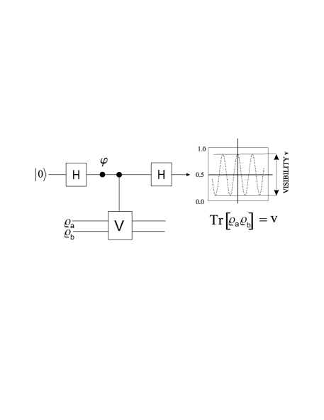
Figure 1: A quantum network for direct estimations of both linear and non-linear functions of state. The probability of finding the control (top line) qubit in state $|0\rangle$ at the output depends on the overlap of the two target states (two bottom lines). Thus estimation of this probability leads directly to an estimation of $\mbox{Tr}\,\varrho_{a}\varrho_{b}=\text{v}=2\,P_{0}-1$.

In order to explain how the network works, let us start with a general observation related to modifications of visibility in interferometry. Consider a typical interferometric set-up for a single qubit: Hadamard gate, phase shift gate $\varphi$, Hadamard gate, followed by a measurement in the computational basis (Figure 1). We modify the interferometer by inserting a controlled-$V$ operation between the Hadamard gates, with its control on the single qubit and with $V$ acting on two quantum systems described by $\varrho_{a}$ and $\varrho_{b}$ respectively. The operator $V$ is the swap operator, defined as $V|\alpha\rangle_{A}|\beta\rangle_{B}=|\beta\rangle_{A}|\alpha\rangle_{B}$, for any pure states $|\alpha\rangle_{A}$ and $|\beta\rangle_{B}$. The action of the controlled-$V$ on $\varrho_{a}\otimes\varrho_{b}$ modifies the interference pattern by the factor

$$\text{v}=\mbox{Tr}\,V\left(\varrho_{a}\otimes\varrho_{b}\right)=\mbox{Tr}\,\varrho_{a}\varrho_{b},$$

where v is the new visibility. The observed modification of the visibility gives an estimate of $\mbox{Tr}\,(\varrho_{a}\varrho_{b})$, i.e. the overlap between states $\varrho_{a}$ and $\varrho_{b}$. The probability of finding the control qubit in state $|0\rangle$ at the output, $P_{0}$, is related to the visibility by $\text{v}=2\,P_{0}-1$. The above network is one of the main ingredients for our discussion in the next section, we redefine it as follows:

Definition 3

Let $n$ be an integer number. The following quantum network with $2n+1$ qubits is called estimation network and is denoted by $E_{n}:$

$$(H^{1}\otimes I^{n}\otimes I^{n})\circ(\mbox{ctrl-}V)\circ(H^{1}\otimes I^{n}\otimes I^{n})\,.$$

3 Quantum Languages

We start by introducing a simple language in ${}^{*}\mathrm{BQP}$ and we build up towards more interesting languages in ${}^{*}\mathrm{QCMA}$ and ${}^{*}\mathrm{QMA}$. In what follows we say that a language $L$ in $\Phi_{\infty}$ or $\Omega_{\infty}$ belongs to a complexity class ${}^{*}C$ iff there exists a small real number $\epsilon$ such that the corresponding partial decision problem $P_{L,\epsilon}$ lies in ${}^{*}C$.

Example 4

Let $f:\mathbb{N}\rightarrow\mathbb{N}$ be a function such that for all $n$ we have $f(n)\leq n$. The quantum language $L_{1}$ defined below belongs to ${}^{*}\mathrm{BQP}:$

$$L_{1}=\{\;|\phi\rangle\in\Phi_{\infty}\;:\;\mbox{The state of the first $f(\ell(|\phi\rangle))$ qubits of $|\phi\rangle$ is pure}\}\,.$$

• Proof

  Let $\varrho$ be the state of the first $m=f(\ell(|\phi\rangle))$ qubits of $|\phi\rangle$ (this can be prepared by tracing out the rest of the qubits in $|\phi\rangle$) and apply $E_{m}$ to $|0\rangle\otimes\varrho\otimes\varrho$. The probability of observing $0$ in the first register is :

  $$P_{0}=\frac{\mbox{Tr}\,(\varrho^{2})+1}{2}\,.$$

  If $\varrho$ is pure, then $P_{0}=1$. If $\varrho$ is mixed, then $1/2<P_{0}<1$. Hence, in order to check that $\varrho$ is indeed pure we need to run $E_{m}$ for a polynomial number of times $M=\mathrm{poly}(\ell(|\phi\rangle))$ and measure the state of the control qubit. In this case $P_{0}=(\frac{\mbox{Tr}\,(\varrho^{2})+1}{2})^{M}$, which will be equal to $1$ if $\varrho$ is pure or tend exponentially to $0$ if $\varrho$ is mixed. The probability of accepting $\varrho$ as pure when it is in fact mixed is thus exponentially small on the number of runs of $E_{m}$. Therefore the following polynomial-time uniformly generated family of quantum circuits $\{C_{n}\}$ satisfies the condition of the definition 1, and will do the job (Figure 2):

  $$C_{m}=T_{M,1}\circ(E_{m}\otimes E_{m}\otimes\cdots\otimes E_{m})\,.$$

  where $M=\mathrm{poly}(\ell(|\phi\rangle))$ and $T_{M,1}$ is a Toffoli type gate which flips the last qubit if all the first $M$ qubits are equal to $1$. Note that the the number of qubits of each $C_{m}$ is polynomial in $\ell(|\phi\rangle)$.     $\sqcap$$\sqcup$

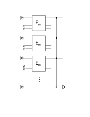
Figure 2: A quantum network for accepting Language $L_{1}$. If $\varrho$ (the state of the first $m$ qubits of $|\phi\rangle$) is pure then the last qubit will be in state $|1\rangle$ with probability one. On the other hand if $\varrho$ is mixed the probability of measuring $1$ in the last qubit decreases exponentially with the number of runs.

The next example is an extension of $L_{1}$ and belongs to ${}^{*}\mathrm{QCMA}$. We can view Definition 2 for accepting a language in ${}^{*}\mathrm{QCMA}$ or ${}^{*}\mathrm{QMA}$ as an interactive protocol consisting of two parties, often called Merlin (with unlimited computational power) and Arthur (with quantum polynomial-time power). Merlin is trying to persuade Arthur that a quantum state $\varrho$ in a given language $L$ satisfies a given property. To this end, he sends Arthur a polynomial-size classical or quantum state as the proof. Each party has access to polynomial number of copies of $\varrho$. Therefore, a protocol to accept the language will be a polynomial-time uniformly generated family of quantum networks with classical or quantum inputs given by Merlin and possibly polynomial number of copies of state $\varrho$.

Example 5

The quantum language $L_{2}$ defined below belongs to ${}^{*}\mathrm{QMCA}:$

$$L_{2}=\{\;|\phi\rangle\in\Phi_{\infty}\;:\;\mbox{$|\phi\rangle$ is separable with respect to two disjoint subsets of qubits}\}\,.$$

In other words every $|\phi\rangle\in L_{2}$ can be written as $|\phi_{1}\rangle\otimes|\phi_{2}\rangle$ where $\ell(|\phi_{1}\rangle)+\ell(|\phi_{2}\rangle)=\ell(|\phi\rangle)$.

• Proof

  Since we assume $|\phi\rangle$ to be pure, it follows that $|\phi_{1}\rangle,|\phi_{2}\rangle$ will be pure as well:

  $$\mbox{Tr}\,(|\phi\rangle\mbox{$\langle\phi|$}^{2}) = \mbox{Tr}\,(|\phi_{1}\rangle\otimes|\phi_{2}\rangle\mbox{$\langle\phi_{1}|$}\otimes\mbox{$\langle\phi_{2}|$}^{2})$$

  $$= \mbox{Tr}\,(|\phi_{1}\rangle\mbox{$\langle\phi_{1}|$}^{2})\mbox{Tr}\,(|\phi_{2}\rangle\mbox{$\langle\phi_{2}|$}^{2})=1$$

  therefore:

  $$\mbox{Tr}\,(|\phi_{1}\rangle\mbox{$\langle\phi_{1}|$}^{2})=\mbox{Tr}\,(|\phi_{2}\rangle\mbox{$\langle\phi_{2}|$}^{2})=1\,.$$

  The protocol for accepting $L_{2}$ uses the network family $\{C_{n}\}$ of the previous example. During the protocol, for $|\phi\rangle\in L_{2}$ Merlin will send a classical binary string of the size $l(|\phi\rangle)$, called subset string, where each $1$ at position $i$ indicates that the $i$th qubit in $|\phi\rangle$ appears in subset ($|\phi_{1}\rangle$). Given a subset string $S$ and the corresponding quantum state $|\phi\rangle$, Arthur apply the simple network of Figure 3 to prepare the corresponding subset state and checks its purity with the proper network $C_{m}$ of the previous example. If Merlin attempts to cheat by sending a false partition the probability of obtaining a $1$ will decrease exponentially with the number of runs.

  

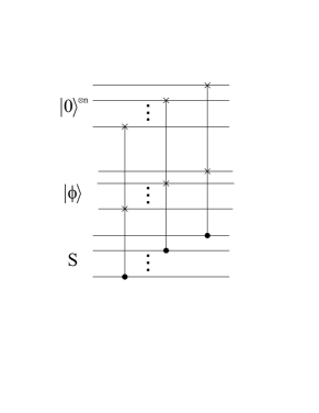
  Figure 3: A quantum network to prepare the corresponding subset state of the state $|\phi\rangle$. In the given classical string $S$, each $1$ at the position $i$ indicates that the $i$th qubit in $|\phi\rangle$ appears in the subset state $|\phi_{1}\rangle$.

Note that any pure state $|\phi\rangle$, entangled with respect to two disjoint subsets of qubits is of the form

$$|\phi\rangle=\sum_{i=1}^{N}c_{i}|\phi_{1}^{i}\rangle\otimes|\phi_{2}^{i}\rangle,$$

where $\sum_{i}|c_{i}|^{2}=1$, $|\phi_{1}^{i}\rangle\otimes|\phi_{2}^{i}\rangle$ are an orthonormal set of states and at least two $c_{i}\neq 0$. On the other hand, a pure separable state is simply $|\varphi_{1}\rangle\otimes|\varphi_{2}\rangle$. Therefore, $|\phi\rangle$ is almost separable if there exists a small real number $\epsilon^{\prime}$ and a $1\leq j\leq N$ such that $|c_{j}|=1-\epsilon^{\prime}$. If $\epsilon^{\prime}\leq\epsilon/2$, where $\epsilon$ is the parameter defining the illegal region of $L_{2}$, $|\phi\rangle$ is undecidable.

$\sqcap$$\sqcup$

Example 6

The quantum language $L_{3}$ defined below belongs to ${}^{*}\mathrm{QMA}:$

$$L_{3}=\{\;\varrho\in\Omega_{\infty}\;:\;\varrho\;\mbox{is an entangled state}\}.$$

• Proof

  A quantum state is said to be entangled if it cannot be written in the form

  $$\varrho_{123...N}=\sum_{\ell}C_{\ell}\varrho^{\ell}_{1}\otimes\varrho^{\ell}_{2}\otimes\varrho^{\ell}_{3}\otimes\ldots\otimes\varrho^{\ell}_{N},$$

  where $\varrho^{\ell}_{j}$ is the state of subsystem $j$, and $\sum_{\ell}C_{\ell}=1$. Checking that a generic $\varrho_{123...N}$ is separable is a hard problem. However, it is possible to construct entanglement witnesses that detect the entanglement in specific entangled states, provided that the state is known. An entanglement witness $W$  [15, 12] is an operator with non-negative expectation value on all separable states, and for which there exists an entangled state such that the expectation value of the witness on that state is negative. Therefore, if Merlin wants to persuade Arthur that a given state $\varrho$ is entangled, it is sufficient for him to send Arthur the respective entanglement witness.

  Merlin cannot send the operator $W$ directly as a physical state because even though $W$ is an operator in the density operators’ Hilbert space, it will not be a valid state in general. So, during the protocol for $|\phi\rangle\in L_{3}$, Merlin will send $W$ as a set of density operators $\varrho_{1},...,\varrho_{k}$ (each of the dimension of $|\phi\rangle$) and a classical string of $k$ real numbers $c_{i}$, such that $W=\sum_{i}c_{i}\varrho_{i}$. Note that based on the construction of a generic $W$ in [12], the number of $\varrho_{i}$’s is polynomial in $\ell(|\varrho\rangle)$ and $c_{i}$’s are polynomial computable real numbers.

  Now, Arthur uses $\varrho_{i}$ and $|\phi\rangle$ as inputs to the proper $C_{m}$ and computes $\mbox{Tr}\,(\varrho_{i}|\phi\rangle)$, for each $i$. Using these expectation values and numbers $c_{i}$, Arthur can estimate

  $$\mbox{Tr}\,(\sum_{i}c_{i}\varrho_{i}|\phi\rangle)=\mbox{Tr}\,(W|\phi\rangle)\,.$$

  If he obtains a negative value, he knows that $|\phi\rangle$ is entangled. Also, in order to check that Merlin did send him an entanglement witness, he can prepare the basis of separable states (with polynomial-size) and check that the expectation value on these states is non-negative.

  $\sqcap$$\sqcup$

To introduce the following language we need few definitions from [8]. Kashefi et al. studied the relation between preparing a set of quantum states and constructing the reflection operators about those states. We begin by the following natural definition of the “easy” states and operators:

Definition 7

A unitary operator $U$ on $n$ qubits is polynomial-time computable (easy), if there exists a network approximately implementing $U$ with polynomial-size in $n$. An $n$-qubit state $|\phi\rangle$ is defined to be polynomial-time preparable (easy), if there exists an easy operator $U$ on ${\rm poly}(n)$ qubits such that $U|0\rangle=|\phi\rangle$.

It is well-known that if a state $|\phi\rangle$ is easy, then the reflection operator about that state, $2|\phi\rangle\mbox{$\langle\phi|$}-I$, is easy (Problem $6.2(1)$ in [14]). The inverse statement is called the Reflection Assumption: “if the reflection about a state is easy, the state itself is easy” and it is known that:

Lemma 8

[8] If there exists a quantum one-way function, then exists a counter-example to the Reflection Assumption.

The next quantum language is concerned with reflection operators:

Example 9

The quantum language $L_{4}$ defined below belongs to ${}^{*}\mathrm{QCMA}$:

$$L_{4}=\{\;|\phi\rangle\in\Phi_{\infty}\;:\;\mbox{The operator $\;\;2|\phi\rangle\mbox{$\langle\phi|$}-I\;\;$ is polynomial-time computable}\}\,.$$

• Proof

During the protocol, for $|\phi\rangle\in L_{4}$ Merlin will send a classical description of the polynomial-size quantum network implementing the reflection operator $R_{\phi}=2|\phi\rangle\mbox{$\langle\phi|$}-I$. Arthur prepares an arbitrary state $|\xi_{i}\rangle$ (unknown to Merlin), which can always be written as:

$$|\xi_{i}\rangle=\alpha|\phi\rangle+\beta|\phi^{\perp}\rangle$$

and applies $R_{\phi}$ to a copy of $|\xi\rangle$, obtaining the output state

$$|\xi_{o}\rangle=\alpha|\phi\rangle-\beta|\phi^{\perp}\rangle\,.$$

Then he uses the network $E_{m}$ with $m=\ell{|\phi\rangle}$ to compute the following values unknown to Merlin:

$$\langle\xi_{i}|\phi\rangle = \mid\alpha\mid^{2}\,,$$ (1)

$$\langle\xi_{o}|\phi\rangle = \mid\alpha\mid^{2}\,,$$ (2)

$$\langle\xi_{o}|\xi_{i}\rangle = \left|\mid\alpha\mid^{2}-\mid\beta\mid^{2}\right|\,,$$ (3)

and he repeats this procedure for $M=\mathrm{poly}(\ell(|\phi\rangle))$ different $|\xi_{i}\rangle$. Arthur will accept $|\phi\rangle$ iff at each run of the above procedure the value of $\alpha$ obtained from Equation $1$ satisfies Equation $2$ and $3$.

Now assume that $|\phi\rangle$ is far from all elements of $L_{4}$, i.e. the reflection operator about $|\phi\rangle$ is not easy, and that Merlin attempts to cheat by sending the description of a polynomial-size network $N$, where $N\neq R_{\phi}$. Following the above strategy, when Arthur applies $N$ to $|\xi_{i}\rangle=\alpha|\phi\rangle+\beta|\phi^{\perp}\rangle$ he will obtain a state of the form $|\xi_{o}\rangle=\alpha^{\prime}|\phi\rangle+\beta^{\prime}|\phi^{\perp}\rangle$. If now he computes the values for the Equation $1$, $2$ and $3$, he will get

$$\langle\xi_{i}|\phi\rangle = \mid\alpha\mid^{2}\,,$$

$$\langle\xi_{o}|\phi\rangle = \mid\alpha^{\prime}\mid^{2}\,,$$

$$\langle\xi_{o}|\xi_{i}\rangle = \left|\alpha^{*}\alpha^{\prime}+\beta^{*}\beta^{\prime}\right|\,.$$

If $\mid\alpha\mid^{2}\neq\mid\alpha^{\prime}\mid^{2}$ Arthur will detect the cheating. If on the other hand $\mid\alpha\mid^{2}=\mid\alpha^{\prime}\mid^{2}$, which implies that $\mid\beta\mid^{2}=\mid\beta^{\prime}\mid^{2}$, we have that $\mbox{$\langle\xi_{o}|\xi_{i}\rangle$}=\left|\mid\alpha\mid^{2}+e^{i\theta}\mid\beta\mid^{2}\right|$, where $\theta$ is the relative phase between $\beta$ and $\beta^{\prime}$. Whenever $\theta\neq\pi$, Equation $3$ will not be satisfied and Arthur will detect the cheating.     $\sqcap$$\sqcup$

Another interesting language in close relation to $L_{4}$ is defined below. First we define the notion of a polynomial-time checkable state [20].

Definition 10

We define a state $|\phi\rangle$ to be efficiently checkable if there exits a polynomial-size quantum network implementing the following checking operator:

$$C_{\phi}|\phi\rangle|0\rangle = |\phi\rangle|0\rangle$$

$$C_{\phi}|\psi\rangle|0\rangle = \alpha|\omega\rangle|0\rangle+\beta|\psi\rangle|1\rangle\;\;\mbox{where}$$

$$\forall|\psi\rangle\perp|\phi\rangle\; : \;\alpha=0\,.$$

Example 11

The quantum language $L_{5}$ defined below belongs to ${}^{*}\mathrm{QCMA}$:

$$L_{5}=\{\;|\phi\rangle\in\Phi_{\infty}\;:\;|\phi\rangle\;\mbox{is efficiently checkable}\}.$$

• Proof

  The next lemma shows that $L_{4}=L_{5}$ which implies $L_{5}\in{}^{*}\mathrm{QCMA}$.     $\sqcap$$\sqcup$

Lemma 12

The quantum languages $L_{4}$ and $L_{5}$ are equal.

• Proof

  Denote by ctrl-$R_{\phi}$ the controlled reflection operator which reflects the state of the first register about $|\phi\rangle$ iff the last qubit (the control qubit) is equal to $1$. We show for any state $|\phi\rangle$:

  $$C_{\phi}=I\otimes H\;\circ\;\mbox{ctrl-}R_{\phi}\;\circ\;I\otimes H\,,$$

  and therefore $L_{4}=L_{5}$. It is easy to check:

  $$|\psi\rangle|0\rangle \stackrel{{\scriptstyle I\otimes H}}{{\longrightarrow}} \frac{1}{\sqrt{2}}|\psi\rangle(|0\rangle+|1\rangle)$$

  $$\stackrel{{\scriptstyle\mbox{ctrl-}R_{\phi}}}{{\longrightarrow}} \frac{1}{\sqrt{2}}\{|\psi\rangle|0\rangle+(2\mbox{$\langle\phi|\psi\rangle$}|\phi\rangle-|\psi\rangle|1\rangle)\}$$

  $$\stackrel{{\scriptstyle I\otimes H}}{{\longrightarrow}} \frac{1}{2}\{2\mbox{$\langle\phi|\psi\rangle$}|\phi\rangle)|0\rangle+2(|\psi\rangle-\mbox{$\langle\phi|\psi\rangle$}|\phi\rangle)|1\rangle\}\,.$$

  If $|\psi\rangle\perp|\phi\rangle$ the final state of the above computation is $|\psi\rangle|1\rangle$ as required.     $\sqcap$$\sqcup$

4 Discussion

Following the work of Yamakami [18], we have considered a general framework for quantum machines with quantum states as input. We introduced some quantum languages in this paradigm and showed the corresponding partial decision problems belong to complexity classes ${}^{*}\mathrm{BQP}$, ${}^{*}\mathrm{QCMA}$ and ${}^{*}\mathrm{QMA}$. These quantum languages can also be viewed as quantum property testing of a set of quantum states.

This investigation of quantum properties (quantum languages) is useful for defining new classical languages within the framework of quantum information theory. For instance, if we consider the subset of quantum states that can be prepared in polynomial-time, e.g. with a polynomial-size quantum circuit, we can derive a classical language from the given quantum language. However, it is not clear how to extend a given classical language to its quantum counterpart. As an example of this derivation consider the classical analogue of language $L_{3}$:

$$L^{\prime}_{3}=\{x\in\Sigma^{*}\; : \;x\;\mbox{describes a polynomial-size quantum network}\;U$$

$$\mbox{and}\;U|0\rangle\;\mbox{is an entangled state}\}\,,$$

which belongs to $\mathrm{QMA}$.

Recently, few complete languages for $\mathrm{QCMA}$ and $\mathrm{QMA}$ have been introduced. Finding complete languages for ${}^{*}\mathrm{QCMA}$ and ${}^{*}\mathrm{QMA}$ would also be very interesting, but it is so far an open problem.

References

- [1] D. Aharonov and O. Regev. A lattice problem in quantum NP. In Proceedings of FOCS’03 – Symposium on Foundations of Computer Science, page 210, 2003.
- [2] C. Moura Alves, P. Horodecki, D. K. L. Oi, L. C. Kwek, and A. Ekert. Direct estimation of functionals of density operators by local operations and classical communication. Phys. Rev. A, 68:032306, 2003.
- [3] H. Buhrman, L. Fortnow, I. Newman, and H. Röhrig. Quantum property testing. In Proceedings of the fourteenth annual ACM-SIAM symposium on Discrete algorithms, page 480, 2003.
- [4] D. Deutsch. Quantum computational networks. Proc. Roy. Soc. Lond A, 425:467, 1989.
- [5] A. Ekert, C. Moura Alves, D. K. L. Oi, M. Horodecki, P. Horodecki, and L. C. Kwek. Direct estimations of linear and non-linear functionals of a quantum state. Phys. Rev. Lett., 88:217901, 2002.
- [6] K. Friedl, F. Magniez, M. Santha, and P. Sen. Quantum testers for hidden group properties. In Proceedings of the 28th International Symposium on Mathematical Foundations of Computer Science, volume 2747, page 419. LNCS, 2003.
- [7] D. Janzing, P. Wocjan, and T. Beth. Identity check is QMA-complete. arXiv.org e-Print quant-ph/0305050, 2003.
- [8] E. Kashefi, H. Nishimura, and V. Vedral. On quantum one-way permutations. Quantum Information and Computation, 2:379, 2002.
- [9] J. Kempe and O. Regev. 3-local hamiltonian is QMA-complete. Quantum Computation and Information, 3:258, 2003.
- [10] A. Kitaev. Quantum NP. Public Talk at AQIP’99: the 2nd Workshop on Algorithms in Quantum Information Processing, 1999.
- [11] E. Knill. Quantum randomness and nondeterminism. arXiv.org e-Print quant-ph/9610012, 1996.
- [12] M. Lewenstein, B. Kraus, J. I. Cirac, and P. Horodecki. Optimization of entanglement witnesses. Phys. Rev. A, 62:52310, 2000.
- [13] M.A. Nielsen and I. Chuang. Programmable quantum gate arrays. Phys. Rev. Letters, 79:321, 1997.
- [14] M.A. Nielsen and I.L. Chuang. Quantum Computation and Quantum Information. Cambridge University Press, Cambridge, 2000.
- [15] B. Terhal. A family of indecomposable positive linear maps based on entangled quantum states. Lin. Alg. Appl., 323:61, 2001.
- [16] J. Watrous. Succinct quantum proofs for properties of finite groups. In Proceedings of FOCS’2000 – Symposium on Foundations of Computer Science, page 537, 2000.
- [17] P. Wocjan, D. Janzing, and T. Beth. Two QCMA-complete problems. arXiv.org e-Print quant-ph/0305090, 2003.
- [18] T. Yamakami. Quantum NP and a Quantum Hierarchy. In Proceedings of 2nd IFIP International Conference on Theoretical Computer Science, page 323, 2002.
- [19] A. C. C. Yao. Quantum circuit complexity. In Proceedings of FOCS’93 – Symposium on Foundations of Computer Science, page 352, 1993.
- [20] The notion of efficiently checkable state and its relation to language has been mentioned to us by Frederic Magniez.