Combinatorics and Optimisation Master of Mathematics

Classical Cryptosystems In A Quantum Setting

Chapter 1 Introduction To Public Key Cryptography

Cryptography has been an area of mathematical study for centuries. Historically, the study of cryptography focused on the design of systems that provide secret communication over an insecure channel. Recently, individuals, corporations, and governments have started to demand privacy, authenticity, and reliability in all sorts of communication, from online shopping to discussions of national secrets. As a result, the goals of cryptography have become more all-encompassing; now, cryptography might better be defined as the design of systems that need to withstand any malicious attempts to abuse them. This thesis will focus on modern algorithms and techniques for confidentiality, which are also known as encryption schemes. However, the purposes of cryptography include not only secret or confidential communication, but also authentication of the entities involved in the communication, authentication of the data transmitted by those entities, and many others.

The oldest encryption schemes are known as symmetric key or secret key systems. Such systems consist of two main algorithms: an encryption algorithm, which allows one entity to encrypt or “scramble” data, and a decryption algorithm, which allows another entity to decrypt or “unscramble” data. Each of these algorithms has an input called a key, which dictates some aspect of the algorithm’s behaviour. In order for two entities (historically known as Alice and Bob) to exchange data securely, they must first share a secret key between them. If Bob wishes to send Alice a message, he uses the secret key with the encryption algorithm to encrypt the message. He sends the encrypted message (called the ciphertext) to Alice, and she uses the secret key with the decryption algorithm to decrypt the ciphertext and recover the original message. Since an eavesdropper (Eve) does not know the secret key, she should not be able to determine what the original message was.

A physical analogy of a symmetric key scheme is often given in terms of boxes and padlocks. Suppose Alice and Bob each have a copy of a key for a padlock. If Bob wishes to send Alice a message, he writes the message on a piece of paper and places it in a box. He then uses his copy of the key to lock the box with the padlock, and he sends the locked box to Alice. When she receives it, she uses her copy of the key to unlock the padlock, she opens the box, and she reads the message. If Eve finds the locked box, however, she cannot open the padlock because she does not have a copy of the key.

Symmetric key encryption schemes are well-suited to many applications. They tend to be very efficient in time and space required for their implementation, and they tend to require only a small amount of key material for a high level of security. The main drawback of such schemes has come to be known as the key distribution problem: if Alice and Bob wish to communicate secretly but have never met, how do they share a secret key? They cannot send a secret key over an insecure channel because Eve might be listening and might learn the key; on the other hand, they do not yet share a secure channel over which to send a secret key. This problem was one of the largest problems in cryptography for many years. Some solutions might be for Alice and Bob to meet in person and agree on a key face-to-face (which is of course impractical if they live far away from one another) or for them to enlist the services of a third party to courier a secret key between them (which implies they both must trust the third party not to reveal the key to anyone). Further, for every pair of parties that wishes to communicate secretly, a unique symmetric key is required; thus the number of symmetric keys in the system grows rapidly.

In the late 1970 s, the mathematicians Diffie and Hellman introduced a new idea: public key cryptography [DH76]. (In fact, a British intelligence researcher had discovered the same idea earlier [Ell70], but his discovery was not made public until later.) Like the secret key systems described above, a public key scheme has two main algorithms for encryption and decryption, each of which has an input called a key. The difference is that the keys used in the two algorithms are not the same. More specifically, Alice generates two keys of her own: a public key, which she shares with everyone (even her enemies) and a private key, which she keeps to herself. If Bob wishes to send Alice a message, he obtains a copy of Alice’s public key, and uses her public key with the encryption algorithm to encrypt the message. He sends the ciphertext to Alice, and she uses her private key with the decryption algorithm to decrypt the ciphertext and recover the original message. Since Eve does not know Alice’s private key, she should not be able to determine what the original message was. In other words, anyone can encrypt a message for Alice, since anyone can obtain Alice’s public key, but once a message is encrypted for her, only Alice can decrypt it with her private key.

Again, we can illustrate the idea of a public key encryption scheme with a physical analogy in terms of boxes and padlocks. Suppose Alice has a number of empty boxes, a number of open padlocks (that can be locked without a key), and a key that opens all of the padlocks. She freely gives out these boxes and open padlocks to anyone who would like them. If Bob wishes to send Alice a message, he writes the message on a piece of paper, gets a box and lock from Alice, and places the message in the box. He then locks the box with the padlock, and he sends the locked box to Alice. When she receives it, she uses her key to unlock the padlock, she opens the box, and she reads the message. If Eve finds the locked box, however, she cannot open the padlock because she does not have a copy of the key. (After he has locked his message in the box, even Bob cannot get the message back out!)

The major advantage of these public key schemes is that they provide a solution to the key distribution problem. Public keys, by design, can be freely distributed to anyone without compromising the security of the system, so if Alice and Bob wish to communicate secretly but they have never met before, they need simply obtain one another’s public keys. There are some disadvantages, in that public key schemes tend to be less efficient and the keys tend to be larger than in secret key systems, but these disadvantages are small compared to the advantages provided by such schemes. There are also ways to use public and secret key schemes together to minimise the disadvantages.

There are several public key cryptosystems that have been proposed, and many have been studied in great detail. The study of these cryptosystems includes studying approaches to breaking them. Breaking a cryptosystem could have many meanings. For example, given only ciphertext, an attacker might try to determine partial or complete information about the corresponding original message. Given only an entity’s public key, an attacker might try to determine partial or complete information about the corresponding private key. There are many variations on the same theme.

Whereas the cryptosystems that are currently in use generally have not been broken, attackers are constantly developing new attacks and improvements in technology are helping to speed up current attacks. Especially worrisome to the field of cryptography are developments in the area of quantum computing, which we will discuss in the next chapter. Even though a quantum computer of a sufficient size has not yet been implemented, the theory of quantum computing indicates that many of the cryptosystems currently in use could easily be broken if this implementation did occur. If a quantum computer is successfully built, we will therefore have to change the cryptosystems we use for encrypted communication so that attackers with quantum computers cannot decrypt it. Further, encrypted messages captured and stored in the past could also be decrypted by a future quantum attacker. Since there is a definite possibility that one day quantum computers will become technologically feasible, we need to prepare for that eventuality by analysing modern cryptosystems with respect to attacks with a quantum computer.

Chapter 2 Introduction To Quantum Computing

This chapter provides an overview of some aspects of quantum computing. For a more complete treatment of the history of the subject and many more details on the ideas discussed in this chapter, see for example [NC00].

2.1 Basic Concepts

The computers that are in widespread use today are sometimes called classical computers. The behaviour of the elements in these computers can be described by the laws of classical physics, that is, those laws that were thought to be accurate around the turn of the twentieth century. However, early in the twentieth century scientists realised that those laws did not accurately describe the behaviour of all systems. For example, objects on an atomic scale behaved differently in experiments than was predicted by classical physics. To more accurately describe these systems, scientists developed a new theory of physics called quantum physics. This theory includes elements of non-determinism, and it more accurately models the behaviour of all systems.

With this new model of physics, a new type of computer has emerged: the quantum computer. A quantum computer is a device that uses the laws of quantum physics to solve problems. There are many ways in which quantum computers could be implemented, some of which are summarised in [NC00]. This thesis will not be concerned with specific implementations, but it is important to note that quantum computers have been implemented successfully, albeit on a small scale. However, regardless of the particular implementation, the behaviour of a quantum computer is governed by a specific set of mathematical rules, namely the laws of quantum physics. A quantum computer can therefore be described completely generally and mathematically.

In a classical computer, information is stored and manipulated in the form of “bits”. Each bit is represented in the computer by an object that exists in one of two states, usually referred to as $0$ and $1$. The computer can manipulate the states of the bits using various logical operations, and it may examine any bit and determine in which of the two states the bit currently exists.

In a quantum computer, information is stored and manipulated in the form of quantum bits, or “qubits”. (Initially, qubits and classical bits seem to be completely different concepts, but as we will see, a bit in a classical computer is really a “restricted” qubit.) A qubit can exist in one of many different states. More specifically, we think of the state of a qubit as a unit vector in a two-dimensional complex vector space. As in any vector space, we could choose any basis and represent the qubit with respect to that basis. However, for each quantum system we model, we will choose a convenient orthonormal basis which we will call the “computational basis”; the computational basis states are denoted $\left|0\right>$ and $\left|1\right>$. In other words, the state of a qubit could be represented as

$$\left|\phi\right>=\alpha\left|0\right>+\beta\left|1\right>$$

where $\alpha$ and $\beta$ are complex numbers. The condition that $\left|\phi\right>$ is a unit vector means that $\left|\alpha\right|^{2}+\left|\beta\right|^{2}=1$. Such a linear combination of basis states is often called a superposition.

We cannot examine a qubit directly to determine its exact state (or in other words, the values $\alpha$ and $\beta$). According to the laws of quantum mechanics, when we measure the qubit, we obtain $\left|0\right>$ with probability $\left|\alpha\right|^{2}$ and $\left|1\right>$ with probability $\left|\beta\right|^{2}$. Further, when such a measurement is made, the state of the qubit “collapses” from its original superposition to either $\left|0\right>$ or $\left|1\right>$, depending on the outcome of the measurement. Apart from the measurement operation, we will restrict our attention to operations that treat the quantum computer as a closed system; that is, we will assume that no information about the state of the system is “leaked” to the apparatus or to an external system.

As we will see in Section 2.3, however, we can manipulate superposition states without extracting information from them. This fact allows us to perform operations that are impossible to implement with a classical computer (even a probabilistic classical computer). For example, as a state is manipulated, the amplitudes of each of the basis states can interfere with each other: two amplitudes of the same sign can combine constructively to increase the probability associated with a particular measurement outcome, or two amplitudes of opposite sign can combine destructively to decrease this probability. The existence of these quantum interference effects is one of the main differences between quantum and classical computers.

Despite these apparent differences, bits and qubits both model a physical system with two orthogonal states. The bits in a classical computer are essentially restricted qubits in that they do not exist in superposition states for long periods of time: they are continually leaking information about their states to external systems. The problems of maintaining coherent superposition states and preventing the computer from coupling with external systems are some of the main challenges that scientists must overcome when implementing a quantum computer.

2.2 Hilbert Space

As described above, we can model the state of a qubit as a vector in a two-dimensional complex vector space. In fact, the state of any quantum mechanical system can be modeled as a vector inside a special kind of vector space called a Hilbert space. For the purposes of this thesis we will restrict our attention to Hilbert spaces of finite dimension, but to describe general quantum systems we need to consider infinite-dimensional spaces. We briefly define a Hilbert space here; for a more complete description the reader may consult for example [Per95]:

Definition 2.1.

A vector space $\mathbb{H}$ is called a Hilbert space if it satisfies the following three properties:

1. For any vectors $u,v\in\mathbb{H}$ and any scalars $\alpha,\beta\in\mathbb{C}$, $\alpha u+\beta v\in\mathbb{H}$.

2. For any vectors $u,v\in\mathbb{H}$ there exists a complex number $\left<\,u\,,\,v\,\right>$ (known as the inner product of $u$ and $v$) the value of which is linear in the first component. Further, $\left<\,u\,,\,v\,\right>$ and $\left<\,v\,,\,u\,\right>$ are complex conjugates of one another, and $\left<\,u\,,\,u\,\right>\geq 0$ with equality if and only if $u=0$.

3. Let $\{u_{m}\}$ be an infinite sequence of vectors in $\mathbb{H}$ and define the norm of $u$ by $\left\|u\right\|=\sqrt{\left<\,u\,,\,u\,\right>}$. If $\left\|u_{m}-u_{n}\right\|\rightarrow 0$ as $m,n\rightarrow\infty$ then there is a unique $u\in\mathbb{H}$ such that $\left\|u_{m}-u\right\|\rightarrow 0$ as $m\rightarrow\infty$. (In other words, any Cauchy sequence of vectors in the space has a limit which is also a vector in the space.)

This last property is known as the completeness property, and it is satisfied by every finite dimensional complex vector space equipped with an inner product. Thus in finite dimensions, every complex inner product space is a Hilbert space [NC00]. (This fact is not true in infinite dimensions.)

Suppose we have two quantum systems, the states of which can be modeled by vectors $\left|\phi\right>\in\mathbb{H}_{m}$ and $\left|\psi\right>\in\mathbb{H}_{n}$ (where $\mathbb{H}_{m}$ and $\mathbb{H}_{n}$ are Hilbert spaces of dimension $m$ and $n$, respectively). To describe the joint state of these systems, we use the “tensor product” of $\left|\phi\right>$ and $\left|\psi\right>$, denoted $\left|\phi\right>\otimes\left|\psi\right>$ or simply $\left|\phi\right>\left|\psi\right>$. This new vector is an element of a larger Hilbert space denoted $\mathbb{H}_{m}\otimes\mathbb{H}_{n}$ (which is in fact defined as the set of all linear combinations of tensor products $\left|\phi\right>\otimes\left|\psi\right>$ with $\left|\phi\right>\in\mathbb{H}_{m}$ and $\left|\psi\right>\in\mathbb{H}_{n}$).

By definition, a tensor product over two vector spaces $V$ and $W$ must satisfy the following properties for all $v,v^{\prime}\in V$, $w,w^{\prime}\in W$, and $\alpha\in\mathbb{C}$:

1. $\alpha(v\otimes w)=(\alpha v)\otimes w=v\otimes(\alpha w)$.

2. $(v+v^{\prime})\otimes w=v\otimes w+v^{\prime}\otimes w$.

3. $v\otimes(w+w^{\prime})=v\otimes w+v\otimes w^{\prime}$.

Also, if $A$ is a linear operator on $V$ and $B$ is a linear operator on $W$, then we can define the linear operator $A\otimes B$ on $V\otimes W$ by

$$(A\otimes B)(v\otimes w)=Av\otimes Bw$$

for all $v\in V$ and $w\in W$.

With these definitions, we are ready to describe more of the basic concepts behind quantum computing.

2.3 Single-Qubit Gates

In a classical computer, we perform computation using circuits of gates connected by wires that carry the bits between the gates. An example of a simple gate in a classical computer is the NOT gate, which maps $0$ to $1$ and $1$ to $0$. An analogous gate in a quantum computer would map $\left|0\right>$ to $\left|1\right>$ and $\left|1\right>$ to $\left|0\right>$. The laws of quantum mechanics state that if we are working in a closed system, we should define the gate’s behaviour on a superposition by extending its behaviour on the basis states linearly. In other words, the quantum NOT gate maps

$$\alpha\left|0\right>+\beta\left|1\right>\longmapsto\beta\left|0\right>+\alpha\left|1\right>.$$

Because a quantum gate is a linear operator on the space of quantum states, we can express it as a matrix with respect to the computational basis. We write the state $\alpha\left|0\right>+\beta\left|1\right>$ in vector form as

$$\begin{pmatrix}\alpha\\ \beta\end{pmatrix}.$$

The NOT gate can then be represented by a matrix X such that for any $\alpha,\beta\in\mathbb{C}$ with $\left|\alpha\right|^{2}+\left|\beta\right|^{2}=1$,

$$\textup{{X}}\begin{pmatrix}\alpha\\ \beta\end{pmatrix}=\begin{pmatrix}\beta\\ \alpha\end{pmatrix}.$$

Thus we must have

$$\textup{{X}}=\begin{pmatrix}0&1\\ 1&0\end{pmatrix}.$$

Any quantum gate that acts on a single qubit can similarly be expressed as a $2\times 2$ matrix. However, the converse is not true: every $2\times 2$ matrix does not define a valid quantum gate. The input and output of a quantum gate are both quantum states, which as mentioned previously are unit vectors in a two-dimensional complex vector space. Thus any quantum gate must be an operator that maps all unit vectors to unit vectors in this vector space; such an operator is called a unitary operator. An equivalent definition of a unitary operator says that U is unitary if and only if $\textup{{U}}^{{\dagger}}\textup{{U}}=\textup{{I}}$, where $\textup{{U}}^{{\dagger}}$ represents the conjugate transpose of U, and I represents the identity operator. It is in fact true that any unitary operator does define a “valid” quantum gate, although not every unitary operation can be performed efficiently in every quantum system; so many of these gates cannot be implemented efficiently.

The unitarity condition on quantum gates implies another important aspect of quantum computation: if we assume that our system is closed, quantum computation is “reversible”. Since the inverse of any unitary operator is also unitary, the inverse operation of a quantum gate is also a quantum gate, and hence given the output of a gate U we can recover the input by applying the valid gate $\textup{{U}}^{\dagger}$.

We will mention two more important single-qubit gates at this time. First, the Hadamard gate is defined by the matrix

$$\textup{{H}}=\frac{1}{\sqrt{2}}\begin{pmatrix}1&\phantom{-}1\\ 1&-1\end{pmatrix},$$

and maps $\left|0\right>$ to $\frac{1}{\sqrt{2}}\bigl{(}\left|0\right>+\left|1\right>\bigr{)}$ and $\left|1\right>$ to $\frac{1}{\sqrt{2}}\bigl{(}\left|0\right>-\left|1\right>\bigr{)}$. Second, the phase gate is defined for any angle $\theta$ by the matrix

$$\textup{{R}}_{\theta}=\begin{pmatrix}1&0\\ 0&e^{i\theta}\end{pmatrix}.$$

This gate leaves the state $\left|0\right>$ unchanged and maps $\left|1\right>$ to $e^{i\theta}\left|1\right>$. It is easy to see that these matrices are unitary, since $\textup{{H}}^{-1}=\textup{{H}}^{\dagger}=\textup{{H}}$ and $\textup{{R}}_{\theta}^{-1}=\textup{{R}}_{\theta}^{\dagger}=\textup{{R}}_{-\theta}$.

2.4 Multiple-Qubit Gates

We can extend the definition of quantum gates to act on $n$ qubits at once. The state of $n$ qubits can be represented as a unit vector in a $2^{n}$-dimensional complex vector space, and again, the only condition on an $n$-qubit gate is that it must be a unitary operator on this vector space. An example of such a gate is the controlled-NOT (or CNOT) gate, whose two inputs are usually called the control and target qubits. The gate can be described as follows:

1. if the control qubit is $\left|0\right>$, the target qubit is not modified, and

2. if the control qubit is $\left|1\right>$, the NOT gate is applied to the target qubit.

There is an interesting result that emphasises the importance of the CNOT gate in quantum computation: any multiple-qubit gate may be constructed using only CNOT gates and single-qubit gates [BBC⁺95].

In a similar fashion we can extend any single-qubit gate to a controlled two-qubit gate. For example, the controlled-$\textup{{R}}_{\theta}$ gate works as follows:

1. if the control qubit is $\left|0\right>$, the target qubit is not modified, and

2. if the control qubit is $\left|1\right>$, the $R_{\theta}$ gate is applied to the target qubit.

In other words, the gate leaves all of the computational basis states unchanged, except for $\left|1\right>\left|1\right>$, which it maps to $e^{i\theta}\left|1\right>\left|1\right>$.

Chapter 3 Introduction To Quantum Algorithms

An algorithm describes a way to solve a particular problem. For example, to solve the problem of dividing one number into another, we could use the algorithm of long division, which consists of many steps that are repeated until we obtain the quotient and remainder. In this section we will present several problems, and describe ways to solve them that involve preparing specific quantum states and applying to them some of the quantum gates defined in Chapter 2. By examining and measuring the output of certain sequences of quantum gates, we can solve a variety of problems.

The quantum algorithms that we present in this chapter are the main tools that we will use in later chapters to analyse classical public key cryptosystems in a quantum setting. As we will see later, many of the cryptosystems we use today are less secure against attacks with a quantum computer since the problems on which these systems are based can be solved in polynomial time with quantum algorithms from this chapter.

3.1 Deutsch’s Problem

Consider the following problem, posed in [Deu85]:

Problem 3.1 (Deutsch’s Problem (DP)).

Given a function $f\colon\{0,1\}\rightarrow\{0,1\}$ determine $f(0)\oplus f(1)$ using only a single evaluation of the function $f$, where $\oplus$ is the componentwise XOR operation.

In other words, we wish to determine with a single evaluation of $f$ whether or not $f$ is a constant function: if $f(0)\oplus f(1)=0$ then $f(0)=f(1)$ so $f$ is constant, and if $f(0)\oplus f(1)=1$ then $f(0)\neq f(1)$ so $f$ is not constant.

If we consider this problem classically, it is impossible to solve: we can determine $f(0)$ or $f(1)$, but without knowing both we cannot solve the problem. (In fact, we cannot determine any information whatsoever that would help us to guess the solution correctly with probability greater than $\frac{1}{2}$.) However, if we consider the problem in a quantum setting and we are given a way to reversibly compute $f$, we can solve it. The solution originally proposed by Deutsch in [Deu85] was modified and improved slightly in [CEMM98] and it is this modified solution that we present here.

To perform a “quantum version” of $f$, we will use an additional qubit (since for a constant function $f$, the mapping $\left|x\right>\longmapsto\left|f(x)\right>$ is not reversible). A typical choice for a reversible implementation of $f$ is the two-qubit unitary operator $\textup{{U}}_{f}$ which performs the transformation

$$\left|x\right>\left|y\right>\longmapsto\left|x\right>\left|y\oplus f(x)\right>$$

for $x,y\in\{0,1\}$.

Suppose that we initialise the second qubit to the state $\frac{1}{\sqrt{2}}\left(\left|0\right>-\left|1\right>\right)$. When we apply $\textup{{U}}_{f}$ to the qubits, by the linearity of quantum operators as discussed above,

$$\textup{{U}}_{f}\Bigl{(}\left|x\right>\tfrac{1}{\sqrt{2}}\bigl{(}\left|0\right>-\left|1\right>\bigr{)}\Bigr{)} =\left|x\right>\tfrac{1}{\sqrt{2}}\bigl{(}\left|0\oplus f(x)\right>-\left|1\oplus f(x)\right>\bigr{)}$$

$$=\left|x\right>(-1)^{f(x)}\tfrac{1}{\sqrt{2}}\bigl{(}\left|0\right>-\left|1\right>\bigr{)}$$

$$=\left((-1)^{f(x)}\left|x\right>\right)\tfrac{1}{\sqrt{2}}\bigl{(}\left|0\right>-\left|1\right>\bigr{)}.$$

Therefore, if we also initialise the first qubit to the state $\frac{1}{\sqrt{2}}\left(\left|0\right>+\left|1\right>\right)$ before applying $\textup{{U}}_{f}$ we obtain

$$\textup{{U}}_{f}\Bigl{(}\tfrac{1}{\sqrt{2}}\bigl{(}\left|0\right>+\left|1\right>\bigr{)}\tfrac{1}{\sqrt{2}}\bigl{(}\left|0\right>-\left|1\right>\bigr{)}\Bigr{)}$$

$$=\tfrac{1}{\sqrt{2}}(-1)^{f(0)}\left|0\right>\tfrac{1}{\sqrt{2}}\bigl{(}\left|0\right>-\left|1\right>\bigr{)}+\tfrac{1}{\sqrt{2}}(-1)^{f(1)}\left|1\right>\tfrac{1}{\sqrt{2}}\bigl{(}\left|0\right>-\left|1\right>\bigr{)}$$

$$=\tfrac{1}{\sqrt{2}}\left((-1)^{f(0)}\left|0\right>+(-1)^{f(1)}\left|1\right>\right)\tfrac{1}{\sqrt{2}}\bigl{(}\left|0\right>-\left|1\right>\bigr{)}.$$

Now we apply the Hadamard gate to the first qubit above:

$$\textup{{H}}\Bigl{(}\tfrac{1}{\sqrt{2}}\left((-1)^{f(0)}\left|0\right>+(-1)^{f(1)}\left|1\right>\right)\Bigr{)}$$

$$=\tfrac{1}{2}(-1)^{f(0)}\bigl{(}\left|0\right>+\left|1\right>\bigr{)}+\tfrac{1}{2}(-1)^{f(1)}\bigl{(}\left|0\right>-\left|1\right>\bigr{)}$$

$$=\tfrac{1}{2}\left((-1)^{f(0)}+(-1)^{f(1)}\right)\left|0\right>+\tfrac{1}{2}\left((-1)^{f(0)}-(-1)^{f(1)}\right)\left|1\right>$$

$$=(-1)^{f(0)}\left|f(0)\oplus f(1)\right>.$$

Apart from the global “phase” of $(-1)^{f(0)}$ that precedes it, the qubit’s state is the correct solution to the problem. Luckily, the laws of quantum physics tell us that the global phase will not affect the outcome of any measurement we perform on the state, and so we can simply measure this qubit and recover the solution $f(0)\oplus f(1)$.

We can summarise the quantum algorithm for Deutsch’s Problem as follows:

Algorithm 3.2 (Solution To DP).

1. Begin with two qubits initialised to the states $\tfrac{1}{\sqrt{2}}\left(\left|0\right>+\left|1\right>\right)$ and $\tfrac{1}{\sqrt{2}}\left(\left|0\right>-\left|1\right>\right)$.

2. Apply the two-qubit quantum gate $\textup{{U}}_{f}$ to the system.

3. Apply the Hadamard gate H to the first qubit.

4. Measure the first qubit and obtain the integer $y$.

5. Return $y$.

3.2 The Hidden Subgroup Problem

Deutsch’s problem is actually a special case of a more general problem:

Problem 3.3 (The Hidden Subgroup Problem (HSP)).

Let $f$ be a function from a finitely generated group $G$ to a finite set $X$ such that $f$ is constant on the cosets of a subgroup $K$ of $G$ and distinct on each coset. Given a quantum network for evaluating $f$ (namely $\textup{{U}}_{f}\colon\left|x\right>\left|y\right>\rightarrow\left|x\right>\left|y\oplus f(x)\right>$) find a generating set for $K$.

In Deutsch’s problem we had $G=\mathbb{Z}_{2}=\{0,1\}$. Using the language of HSP,

1. if $f$ is a constant function, we have $K=\{0,1\}$ since $f$ is constant on $K$ (and there is only one coset of $K$, namely $K$ itself); and

2. if $f$ is not constant, then we have $K=\{0\}$, since $f$ is constant on $K$ and on $K+1=\{1\}$, and distinct on these two cosets.

Thus to solve Deutsch’s problem we wish to determine whether $K=\{0,1\}$ or $K=\{0\}$.

There are many other problems that can be thought of as special cases of HSP. We list two important examples below, and for many more, see [Mos99].

Problem 3.4 (The Order Finding Problem (OFP)).

Given an element $a$ of a finite group $H$, find $r$, the order of $a$.

Let $f\colon\mathbb{Z}\rightarrow H$ be defined by $f(x)=a^{x}$. Then note that

$$f(x)=f(y) \Longleftrightarrow a^{x}=a^{y}$$

$$\Longleftrightarrow a^{x-y}=1$$

$$\Longleftrightarrow x-y\in\{t\cdot r:t\in\mathbb{Z}\}.$$

That is, $f(x)=f(y)$ if and only if $x$ and $y$ are in the same coset of the hidden subgroup $K=r\mathbb{Z}$ of $\mathbb{Z}$. By finding a generator for $K$ we can determine $r$. Thus OFP is a special case of HSP.

Problem 3.5 (The Discrete Logarithm Problem (DLP)).

Given an element $a$ of a finite group $H$ and $b=a^{k}$, find $k$. (This $k$ is called the discrete logarithm of $b$ to the base $a$.)

Suppose the order of $a$ is $r$. Let $f\colon\mathbb{Z}_{r}\times\mathbb{Z}_{r}\rightarrow H$ be defined by $f(x_{1},x_{2})=a^{x_{1}}b^{x_{2}}$. Then note that

$$f(x_{1},x_{2})=f(y_{1},y_{2}) \Longleftrightarrow a^{x_{1}}b^{x_{2}}=a^{y_{1}}b^{y_{2}}$$

$$\Longleftrightarrow a^{x_{1}-y_{1}}b^{x_{2}-y_{2}}=1$$

$$\Longleftrightarrow a^{x_{1}-y_{1}}a^{k(x_{2}-y_{2})}=1$$

$$\Longleftrightarrow(x_{1}-y_{1})+k(x_{2}-y_{2})=0\quad\text{(in $\mathbb{Z}_{r}$)}$$

$$\Longleftrightarrow(x_{1},x_{2})-(y_{1},y_{2})\in\{(-tk,t)\,:\,t\in\mathbb{Z}_{r}\}.$$

That is, $f(x_{1},x_{2})=f(y_{1},y_{2})$ if and only if $(x_{1},x_{2})$ and $(y_{1},y_{2})$ are in the same coset of the hidden subgroup $K=\langle(-k,1)\rangle$ of $\mathbb{Z}_{r}\times\mathbb{Z}_{r}$. By finding a generator for $K$ we can determine $k$. Thus DLP is a special case of HSP.

We mention these two problems in particular because as we will see in the remainder of this thesis, if we have algorithms to solve these problems efficiently, we can break many of the classical cryptosystems that are in widespread use today. There do exist polynomial-time quantum algorithms that solve these problems, and we will discuss these algorithms later. In fact, there exist efficient quantum algorithms that solve the general HSP when the group $G$ is Abelian, as described in [Mos99]. Some work has been done to design algorithms for HSP in non-Abelian groups, although success has been limited. For example, an efficient algorithm was presented in [Ey00] that is able to determine some information about the generator of a hidden subgroup in a dihedral group, but there is no known way to recover the subgroup in polynomial time from this information. In [IMS01] some special cases of the problem were solved in non-Abelian groups, but the general case still remains open.

We now introduce one of the most important ingredients in many quantum algorithms: the Quantum Fourier Transform.

3.3 The Quantum Fourier Transform

The Quantum Fourier Transform (QFT) provides a way to estimate parameters that are encoded in a specific way in the phases and amplitudes of quantum states. We will begin with a small three-qubit example, and then define the general QFT.

Assume $a$ is an integer, $0\leq a<8$. Now suppose that we are given the three-qubit state

$$\bigl{(}\left|0\right>+e^{2\pi i\frac{a}{2}}\left|1\right>\bigr{)}\bigl{(}\left|0\right>+e^{2\pi i\frac{a}{4}}\left|1\right>\bigr{)}\bigl{(}\left|0\right>+e^{2\pi i\frac{a}{8}}\left|1\right>\bigr{)}$$

(ignoring the normalisation factors) and we wish to find $a$.

We can write $a=4a_{2}+2a_{1}+a_{0}$ where each $a_{j}\in\{0,1\}$ and then rewrite the state as

$$\bigl{(}\left|0\right>+e^{2\pi i(\frac{a_{0}}{2})}\left|1\right>\bigr{)}\bigl{(}\left|0\right>+e^{2\pi i(\frac{2a_{1}+a_{0}}{4})}\left|1\right>\bigr{)}\bigl{(}\left|0\right>+e^{2\pi i(\frac{4a_{2}+2a_{1}+a_{0}}{8})}\left|1\right>\bigr{)}.$$

Recall the Hadamard gate H from Section 2.3 and note that ignoring normalisation factors we could equivalently define it by the map

$$\left|x\right>\longrightarrow\left|0\right>+e^{2\pi i\frac{x}{2}}\left|1\right>$$

for $x\in\{0,1\}$. So if we apply $\textup{{H}}^{-1}=\textup{{H}}$ to the first qubit, we obtain $\left|a_{0}\right>$.

Next, we will try to determine $a_{1}$. Consider the following two cases:

1. If $a_{0}=0$, the second qubit is actually in the state $\left|0\right>+e^{2\pi i(\frac{a_{1}}{2})}\left|1\right>$.

2. If $a_{0}=1$, the second qubit is in the state $\left|0\right>+e^{2\pi i(\frac{2a_{1}+1}{4})}\left|1\right>$. In this case, if we apply a $\textup{{R}}_{-\frac{\pi}{2}}$ gate to the qubit, we get

   $$\left|0\right>+e^{2\pi i(\frac{2a_{1}+1}{4})}e^{-i\frac{\pi}{2}}\left|1\right>$$

   $$=\left|0\right>+e^{2\pi i(\frac{a_{1}}{2})}\left|1\right>.$$

Thus we will obtain a common state if we can decide, based on the state of the first qubit, whether or not to apply a $\textup{{R}}_{-\frac{\pi}{2}}$ gate to the second qubit. In other words, we wish to apply a controlled-$\textup{{R}}_{-\frac{\pi}{2}}$ gate to the first and second qubits. After this gate has been applied, our second qubit will be in the state $\left|0\right>+e^{2\pi i(\frac{a_{1}}{2})}\left|1\right>$, and we can apply an H gate to the second qubit to obtain the state $\left|a_{1}\right>$.

Similarly, if we now apply a controlled-$\textup{{R}}_{-\frac{\pi}{4}}$ to the first and third qubits, the third qubit will be in the state $\left|0\right>+e^{2\pi i(\frac{2a_{2}+a_{1}}{4})}\left|1\right>$. Then, applying a controlled-$\textup{{R}}_{-\frac{\pi}{2}}$ to the second and third qubits will put the third qubit into the state $\left|0\right>+e^{2\pi i(\frac{a_{2}}{2})}\left|1\right>$. Finally, we can apply an H gate to the third qubit to obtain $\left|a_{2}\right>$.

The sequence of gates we have described, illustrated in Figure 3.1, implements the transformation

$$\bigl{(}\left|0\right>+e^{2\pi i\frac{a}{2}}\left|1\right>\bigr{)}\bigl{(}\left|0\right>+e^{2\pi i\frac{a}{4}}\left|1\right>\bigr{)}\bigl{(}\left|0\right>+e^{2\pi i\frac{a}{8}}\left|1\right>\bigr{)}\longrightarrow\left|a_{0}\right>\left|a_{1}\right>\left|a_{2}\right>$$

and by reversing the order of the qubits, we obtain the $3$-qubit state

$$\left|a_{2}\right>\left|a_{1}\right>\left|a_{0}\right>\;=\;\left|a\right>.$$

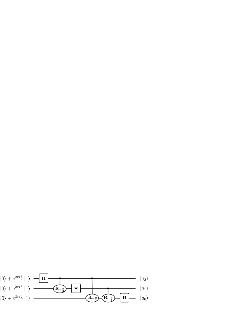
Figure 3.1: A 3-qubit Quantum Fourier Transform

We can generalise this quantum circuit so that if $a$ is an integer with $0\leq a<2^{n}$ and $a=2^{n-1}a_{n-1}+2^{n-2}a_{n-2}+\cdots+2a_{1}+a_{0}$ for $a_{j}\in\{0,1\}$, we can start with the $n$-qubit state

$$\bigl{(}\left|0\right>+e^{2\pi i\frac{a}{2}}\left|1\right>\bigr{)}\bigl{(}\left|0\right>+e^{2\pi i\frac{a}{4}}\left|1\right>\bigr{)}\cdots\bigl{(}\left|0\right>+e^{2\pi i\frac{a}{2^{n}}}\left|1\right>\bigr{)}$$ (3.1)

and transform it into the state

$$\left|a_{n-1}\right>\left|a_{n-2}\right>\cdots\left|a_{1}\right>\left|a_{0}\right>\;=\;\left|a\right>.$$

As pointed out in [Mos99], the start state (3.1) can be rewritten as

$$\sum_{x=0}^{2^{n}-1}e^{2\pi ix\frac{a}{2^{n}}}\left|x\right>.$$

The states of this form, for $a=0,1,\ldots,2^{n}-1$ are called the Fourier basis states. The transformation we have discussed in this section therefore maps a state in the Fourier basis to its corresponding state in the computational basis. We call this transformation the inverse QFT; the QFT therefore maps states from the computational basis to the Fourier basis.

We can define the QFT more generally as follows:

Definition 3.6.

For any integer $m>1$, the $m$-bit Quantum Fourier Transform $\textup{{QFT}}_{m}$ acts on the vector space generated by the states

$$\left|0\right>,\left|1\right>,\ldots,\left|m-1\right>$$

and maps

$$\left|a\right>\longmapsto\frac{1}{\sqrt{m}}\sum_{x=0}^{m-1}e^{2\pi ix\frac{a}{m}}\left|x\right>.$$

We have described an efficient implementation of $\textup{{QFT}}_{m}$ in the case where $m$ is a power of $2$, as originally presented in [Cop94]. There are also efficient exact implementations of $\textup{{QFT}}_{m}$ in the case where the prime factors of $m$ are distinct and in $O\!\left(\log m\right)$ [Sho94], or more generally when the prime factors are not necessarily distinct but still in $O\!\left(\log m\right)$ [Cle94]. It was shown in [Kit95] that for arbitrary values of $m$ we can approximate $\textup{{QFT}}_{m}$ efficiently; very recently, it was shown that we can in fact implement $\textup{{QFT}}_{m}$ exactly for arbitrary values of $m$ [MZ03].

We now make some important observations about the QFT. First, if we start in the state $\left|0\right>$ and apply $\textup{{QFT}}_{m}$ we obtain the state

$$\frac{1}{\sqrt{m}}\sum_{x=0}^{m-1}e^{2\pi ix\frac{0}{m}}\left|x\right>$$

$$=\frac{1}{\sqrt{m}}\sum_{x=0}^{m-1}\left|x\right>$$

which is an equally weighted superposition of the $m$ computational basis states.

Also, given the state $\left|\phi\right>=\frac{1}{\sqrt{m}}\sum_{x=0}^{m-1}e^{2\pi ix\omega}\left|x\right>$ where $\omega=\frac{a}{m}$ for some integer $a$, then by definition, if we apply the inverse QFT to $\left|\phi\right>$ we will obtain the state $\left|a\right>$ and we can recover $\omega$ exactly. If, on the other hand, $\omega$ is any real number, we can still use the inverse QFT to obtain an estimate of $\omega$, and we can bound the distance of this estimate from the true value of $\omega$. More precisely:

Theorem 3.7.

Given an integer $m>0$ and the state $\left|\phi\right>=\frac{1}{\sqrt{m}}\sum_{x=0}^{m-1}e^{2\pi ix\omega}\left|x\right>$, where $\omega$ is an any real number, applying $\textup{{QFT}}_{m}^{-1}$ to $\left|\phi\right>$ and measuring the result yields an integer $y$ satisfying the following conditions:

• If $\omega=\frac{a}{m}$ for some integer $a$, then with probability $1$, $y=a$.

• Otherwise, with probability at least $\frac{8}{\pi^{2}}$, $\left|\frac{y}{m}-\omega\right|\leq\frac{1}{m}$.

For a proof of this theorem, see [Che03].

3.4 Solving A Special Case Of The Hidden Subgroup Problem

We first consider the task of solving HSP where $G=\mathbb{Z}$; that is, $f$ is a function from $\mathbb{Z}$ to some finite set $X$, and $f(x)=f(y)$ if and only if $x-y\in r\mathbb{Z}$ for some fixed (unknown) integer $r$. We will call this special case of HSP the Integer Hidden Subgroup Problem (IHSP).

We choose an integer $n\geq\log\left|X\right|$ and an integer $m$ which is a power of $2$, and we are given the unitary operator $\textup{{U}}_{f}$ which acts on $\mathbb{H}_{m}\otimes\mathbb{H}_{n}$ and maps $\left|x\right>\left|y\right>\longmapsto\left|x\right>\left|y\oplus f(x)\right>$. We can then implement the following algorithm, which will form the core of an algorithm to solve IHSP:

Algorithm 3.8 (Core Of Solution To IHSP).

1. Start in the state $\left|0\right>\left|0\right>\in\mathbb{H}_{m}\otimes\mathbb{H}_{n}$.

2. Apply $\textup{{QFT}}_{m}$ to the first register.

3. Apply $\textup{{U}}_{f}$ to the system.

4. Apply $\textup{{QFT}}_{m}^{-1}$ to the first register.

5. Measure the first register to obtain the integer $y$.

6. Return $y$.

We now have the following well-known result (see for example [NC00]):

Proposition 3.9.

After Step 3 of Algorithm 3.8, our system is in the state

$$\left|\phi\right>=\frac{1}{\sqrt{rm}}\sum_{k=0}^{r-1}\left(\sum_{x=0}^{m-1}e^{2\pi ix\frac{k}{r}}\left|x\right>\right)\left|\psi_{k}\right>$$

where $\smash{\left|\psi_{k}\right>=\frac{1}{\sqrt{r}}\sum\limits_{j=0}^{r-1}e^{-2\pi ij\frac{k}{r}}\left|f(j)\right>}$.

Proof.

After Step 2 of Algorithm 3.8, our system is in the state $\frac{1}{\sqrt{m}}\sum_{x=0}^{m-1}\left|x\right>\left|0\right>$, and applying $\textup{{U}}_{f}$ in Step 3 produces the state $\frac{1}{\sqrt{m}}\sum_{x=0}^{m-1}\left|x\right>\left|f(x)\right>$. We will show that this state is in fact equal to $\left|\phi\right>$. Note that

$$\left|\phi\right> =\frac{1}{r\sqrt{m}}\sum_{k=0}^{r-1}\left(\sum_{x=0}^{m-1}e^{2\pi ix\frac{k}{r}}\left|x\right>\right)\sum_{j=0}^{r-1}e^{-2\pi ij\frac{k}{r}}\left|f(j)\right>$$

$$=\frac{1}{r\sqrt{m}}\sum_{x=0}^{m-1}\sum_{j=0}^{r-1}\left(\sum_{k=0}^{r-1}e^{2\pi i\frac{k}{r}(x-j)}\right)\left|x\right>\left|f(j)\right>.$$ (3.2)

Now fix $x$ and $j$, and consider the coefficients $c_{k}=e^{2\pi i\frac{k}{r}(x-j)}$ for $0\leq k<r$. There are two cases:

1. If $x\equiv j\pmod{r}$ then $\frac{k}{r}(x-j)$ is an integer for all $k$, so each of the $c_{k}$ is $1$, and the sum of the $c_{k}$ is $r$. In this case, we say that there is constructive interference between the coefficients.

2. If $x\not\equiv j\pmod{r}$, consider $c_{1}=e^{2\pi i\frac{1}{r}(x-j)}$. Note that $c_{1}^{\;r}-1=0$, and since $c_{1}^{\;r}-1=(c_{1}-1)(1+c_{1}+\cdots+c_{1}^{\;r-1})$ and $c_{1}-1\neq 0$, it must be true that $1+c_{1}+\cdots+c_{1}^{\;r-1}=0$. Furthermore, $c_{1}^{\;k}=c_{k}$ for $0\leq k<r$, so the sum of the $c_{k}$ is $0$. In this case we say that there is destructive interference between the coefficients.

Thus from (3.2), we see that

$$\left|\phi\right> =\frac{1}{r\sqrt{m}}\sum_{x=0}^{m-1}\sum_{j=0}^{r-1}\left(\sum_{k=0}^{r-1}c_{k}\right)\left|x\right>\left|f(j)\right>$$

$$=\frac{1}{r\sqrt{m}}\sum_{x=0}^{m-1}\left|x\right>r\left|f(x\bmod{r})\right>$$

$$=\frac{1}{\sqrt{m}}\sum_{x=0}^{m-1}\left|x\right>\left|f(x)\right>$$

since by the periodicity of $f$, $f(x)=f(x\bmod{r})$. Therefore the result is proven. ∎

So after Step 3 our system is in the state $\frac{1}{\sqrt{m}}\sum_{k=0}^{r-1}\bigl{(}\sum_{x=0}^{m-1}e^{2\pi ix\frac{k}{r}}\left|x\right>\bigr{)}\left|\psi_{k}\right>$. Letting $\omega=\frac{k}{r}$, by Theorem 3.7 and by linearity we can see that with probability at least $\frac{8}{\pi^{2}}$, applying $\textup{{QFT}}_{m}^{-1}$ to the first register and measuring the result yields an integer $y_{k}$ such that $\left|\frac{y_{k}}{m}-\frac{k}{r}\right|\leq\frac{1}{m}$, where $k$ is chosen at random from $\{0,1,\ldots,r-1\}$.

We will now make use of a theorem from the theory of continued fractions. Given any real number $\lambda$, we can use the theory of continued fractions to compute a sequence of rational numbers called “convergents” that approximate $\lambda$ with increasing precision. If $\lambda$ is positive and rational (say $\lambda=\frac{x}{m}$ for positive integers $x$ and $m$) we have the following result (see for example [Ros93]):

Theorem 3.10.

Let $x$, $m$, $k$, and $r$ be positive integers, with

$$\left|\frac{x}{m}-\frac{k}{r}\right|<\frac{1}{2r^{2}}$$

Then $\frac{k}{r}$ appears as a convergent in the continued fraction expansion of $\frac{x}{m}$.

There exist efficient algorithms to compute the continued fraction expansion of $\frac{x}{m}$, as described for example in [Kob94]. Clearly there exists at most one fraction $\frac{a}{b}$ with $b\leq r$ such that $\left|\frac{x}{m}-\frac{a}{b}\right|\leq\frac{1}{2r^{2}}$, so when we find such a convergent $\frac{a}{b}$, we know that $\frac{a}{b}=\frac{k}{r}$ and we can stop computing convergents. The continued fractions algorithms guarantee that we will have to compute at most $O\!\left(\log{m}\right)$ convergents before we can stop.

So by setting $x$ equal to our measurement output $y_{k}$ and running these algorithms, provided we have chosen $m>2r^{2}$, we can efficiently find a fraction $\frac{a}{b}=\frac{k}{r}$.

Combining Algorithm 3.8 and Theorem 3.10, we obtain an efficient probabilistic quantum algorithm to solve IHSP if we have a bound on the size of $r$:

Algorithm 3.11 (Solution To IHSP When $r$ Is Bounded).

1. Choose an integer $m>2r^{2}$.

2. Repeat Algorithm 3.8 two times to obtain two values $y_{k_{1}},y_{k_{2}}$.

3. Use the continued fractions algorithm to obtain fractions $\frac{a_{1}}{b_{1}},\frac{a_{2}}{b_{2}}$ such that$b_{1},b_{2}\leq\sqrt{\frac{m}{2}}$ and

   $$\left|\frac{y_{k_{1}}}{m}-\frac{a_{1}}{b_{1}}\right|,\left|\frac{y_{k_{2}}}{m}-\frac{a_{2}}{b_{2}}\right| \leq\frac{1}{m}.$$

   If two such fractions cannot be found, return FAIL.

4. Let $t=\operatorname{lcm}(b_{1},b_{2})$. If $t>\sqrt{\frac{m}{2}}$, return FAIL.

5. If $f(0)\neq f(t)$, return FAIL.

6. Return $t$.

Theorem 3.12.

Algorithm 3.11 finds the correct value of $r$ with probability at least $\frac{32}{\pi^{4}}$. If it does not return FAIL, it returns a multiple of $r$.

Proof.

We run Algorithm 3.8 twice independently, obtaining results $y_{k_{1}}$ and $y_{k_{2}}$. The values $\frac{y_{k_{1}}}{m}$ and $\frac{y_{k_{2}}}{m}$ are estimates of $\frac{k_{1}}{r}$ and $\frac{k_{2}}{r}$, respectively.

By Theorem 3.7, $\left|\frac{y_{k_{i}}}{m}-\frac{k_{i}}{r}\right|\leq\frac{1}{m}$ with probability at least $\frac{8}{\pi^{2}}$ for $i=1$, and independently for $i=2$. The probability that the inequality is satisfied for both $i=1$ and $i=2$ is therefore at least $\frac{64}{\pi^{4}}$. If this is the case, then since $m>2r^{2}$, by Theorem 3.10 the continued fractions algorithm will successfully find fractions $\frac{a_{1}}{b_{1}}$ and $\frac{a_{2}}{b_{2}}$ that satisfy the conditions in Step 3. Thus with probability at least $\frac{64}{\pi^{4}}$ we will have found $\frac{a_{i}}{b_{i}}=\frac{k_{i}}{r}$ for $i=1,2$.

Now note that $\gcd(k_{i},r)$ is not necessarily $1$ because $\frac{a_{i}}{b_{i}}$ could be the reduced form of $\frac{k_{i}}{r}$. It is true however that $b_{i}=\frac{r}{\gcd(k_{i},r)}$, so $\operatorname{lcm}(b_{1},b_{2})=\frac{r}{\gcd(k_{1},k_{2},r)}$. If, whenever we have measured a $0$ we replace it by $r$ (for mathematical convenience) we can treat $k_{1}$ and $k_{2}$ as having been selected uniformly at random from the integers between $1$ and $r$; so $k_{1}$ and $k_{2}$ are coprime with probability at least $\frac{1}{2}$ [CEMM98]. In this case, $\operatorname{lcm}(b_{1},b_{2})=r$ as desired. Thus the algorithm finds the correct value of $r$ with probability at least $\left(\frac{64}{\pi^{4}}\right)\left(\frac{1}{2}\right)=\frac{32}{\pi^{4}}$.

The final test in Step 5 checks to make sure that $t$ is a multiple of $r$. Thus the algorithm either returns FAIL or a multiple of $r$. ∎

If we do not have a bound on $r$ to begin with, we can guess at an initial value of $m$, and repeat Algorithm 3.11 three times, say. If all three repetitions return FAIL, we can assume that our $m$ is not large enough, double it, and try again. Eventually, we will obtain an $m>2r^{2}$, and with high probability, one of the repetitions of the algorithm for that value of $m$ will succeed. The number of iterations of this process that are required to ensure $m>2r^{2}$ is polynomial in $\log{r}$.

Thus we have an efficient quantum algorithm to solve IHSP. It should be noted that if $f$ is given to us as a “black box”, there is no efficient classical algorithm to solve IHSP: it is a problem for which an efficient quantum algorithm exists but for which no known efficient classical algorithm exists.

3.5 Solving The Order Finding Problem

Given an element $a$ of a group $H$, to solve OFP we must compute $r$, the order of $a$. As illustrated in Problem 3.4, OFP is a special case of IHSP where $f(x)=a^{x}$. Thus, the algorithm we have described in Section 3.4 allows us to solve OFP in polynomial time. A polynomial-time quantum algorithm to solve OFP was first proposed in [Sho94].

3.6 Solving The Factoring Problem

In this section, we describe how to find a non-trivial factor of an integer in polynomial time using a quantum computer. Given a polynomial-time algorithm to solve OFP we can use a classical reduction to develop an algorithm that allows us to find a non-trivial factor of an integer in polynomial time. This reduction was first described by Miller in [Mil76]. The idea of solving the factoring problem using the polynomial-time quantum algorithm for OFP and Miller’s reduction was proposed in [Sho94]. The resulting quantum factoring algorithm has become the most famous quantum algorithm.

We present a sketch of Miller’s reduction. Suppose we wish to factor a positive integer $n$. First, we assume that $n$ is odd, since factors of $2$ are easy to detect. We also assume that $n$ is not a prime power, since there are efficient classical algorithms to determine the factors of $n$ in this case. Consider the following algorithm:

Algorithm 3.13 (Finding A Non-Trivial Factor).

1. Choose an integer $a$ at random from $\{0,1,\ldots,n-1\}$.

2. Let $s=\gcd(a,n)$. If $s>1$ then return $s$. Otherwise, $a\in\mathbb{Z}_{n}^{*}$. (Recall that $\mathbb{Z}_{n}^{*}$ is the multiplicative group of all integers (modulo $n$) that are coprime with $n$.)

3. Apply Algorithm 3.11 three times with $m>2n^{2}$ to attempt to determine the order of $a$ in $\mathbb{Z}_{n}^{*}$. If all three results are FAIL, return FAIL. Otherwise, take $r$ to be the minimum non-FAIL output.

4. If $r$ is odd, return FAIL.

5. Let $t=\gcd(a^{r/2}-1,n)$. If $t=1$, return FAIL.

6. Return $t$.

Theorem 3.14.

Algorithm 3.13 correctly returns a non-trivial factor of $n$ with probability at least $\frac{1}{3}$.

Proof.

For any integer $a\in\{0,1,\ldots,n-1\}$ which is coprime with $n$ and whose order in $\mathbb{Z}_{n}^{*}$ is $r$, we know that

$$a^{r} \equiv 1\pmod{n}$$

$$a^{r}-1 \equiv 0\pmod{n}$$

$$(a^{r/2}-1)(a^{r/2}+1) \equiv 0\pmod{n}\quad\mbox{(if $r$ is even)}.$$

Since $r$ is the order of $a$, we know that $a^{r/2}-1\not\equiv 0\pmod{n}$. So if

1. $r$ is even, and

2. $a^{r/2}+1\not\equiv 0\pmod{n}$,

then $t=\gcd(a^{r/2}-1,n)$ must be a non-trivial factor of $n$.

We now show that a randomly selected $a$ satisfies both of these conditions with probability at least $1-(\frac{1}{2})^{k-1}$, where $k$ is the number of distinct odd prime factors of $n$. Let $n=\prod_{i=1}^{k}p_{i}^{e_{i}}$ where the $p_{i}$ are distinct odd primes, and let $r_{i}$ be the order of $a$ in $\mathbb{Z}_{p_{i}^{e_{i}}}^{*}$. Then $r$ is the least common multiple of the $r_{i}$. Consider the multiplicity of $2$ in the prime factorisation of each $r_{i}$.

1. If each of these multiplicities is $0$ (ie. each $r_{i}$ is odd) then $r$ is odd.

2. If each of these multiplicities is larger than $0$ but they are all equal, then $r_{i}$ does not divide $\frac{r}{2}$ for any $i$, and thus it must be true that $a^{r/2}\equiv-1\pmod{p_{i}^{e_{i}}}$ for each $i$. Then by the Chinese Remainder Theorem, $a^{r/2}\equiv-1\pmod{n}$.

3. Otherwise, there is some $i$ for which $a^{r/2}\equiv 1\pmod{p_{i}^{a_{i}}}$ and thus $a^{r/2}\not\equiv-1\pmod{n}$.

Thus a randomly selected $a$ will fail to satisfy both required conditions if and only if the multiplicities of $2$ in the prime factorisations of the $r_{i}$ are all the same. By the Chinese Remainder Theorem, there is a one-to-one correspondence between $\mathbb{Z}_{n}^{*}$ and the set $\{(x_{1},\ldots,x_{k}):x_{i}\in\mathbb{Z}_{p_{i}^{e_{i}}}^{*},1\leq i\leq k\}$. Thus selecting an $a$ at random from $\mathbb{Z}_{n}^{*}$ is the same as selecting a $k$-tuple at random from the above set. For each $i$, $\mathbb{Z}_{p_{i}^{e_{i}}}^{*}$ is cyclic since $p_{i}$ is odd; so if we choose a random element $x_{i}$ with order $r_{i}$, the probability of obtaining a particular multiplicity of $2$ in the prime factorisation of $r_{i}$ is at most $\frac{1}{2}$. Thus the probability of obtaining the same multiplicity for each $i$ is at most $(\frac{1}{2})^{k-1}$. In other words, the probability of choosing an appropriate $a$ is at least

$$1-\left(\tfrac{1}{2}\right)^{k-1}.$$ (3.3)

If such an $a$ is chosen, the algorithm will succeed in finding a non-trivial factor of $n$ provided that at least one of the applications of Algorithm 3.11 is successful in correctly determining $r$, the order of $a$ in $\mathbb{Z}_{n}^{*}$. By Theorem 3.12 each individual application of Algorithm 3.11 succeeds with probability at least $\frac{32}{\pi^{4}}$. Thus the probability that at least one of them succeeds is

$$1-\left(1-\left(\tfrac{32}{\pi^{4}}\right)\right)^{3}>\tfrac{2}{3}.$$ (3.4)

Combining (3.3) and (3.4), we see that the probability that the entire algorithm succeeds is at least

$$\left(1-\left(\tfrac{1}{2}\right)^{k-1}\right)\left(\tfrac{2}{3}\right).$$

Since we have assumed $n$ is not a prime power, $k\geq 2$. Thus the probability of success is at least $\left(\frac{1}{2}\right)\left(\frac{2}{3}\right)>\frac{1}{3}.$ ∎

By applying this algorithm recursively, we can split $n$ into its prime factors. We therefore have a polynomial time probabilistic quantum algorithm to solve the factoring problem.

The core of this quantum factoring algorithm has been successfully implemented on a small quantum computer to attempt to factor the integer $15$ into its prime factors ($3$ and $5$). Scientists are still only able to tackle problems with small parameter sizes using the current implementations of quantum computers, but the successful implementation of this and other quantum algorithms indicates that the theory currently being developed can actually be applied to a physical realisation of a quantum computer.

3.7 Solving Another Special Case Of The Hidden Subgroup Problem

Next consider the task of solving HSP where $G=\mathbb{Z}_{p}\times\mathbb{Z}_{p}$; that is, $f$ is a function from $\mathbb{Z}_{p}\times\mathbb{Z}_{p}$ to some finite set $X$, and $f(x_{1},x_{2})=f(y_{1},y_{2})$ if and only if $(x_{1},x_{2})$ and $(y_{1},y_{2})$ are in the same coset of some hidden subgroup $K$ (which is of size $p$). We will call this special case of HSP the Prime Hidden Subgroup Problem (PHSP). In this section we will present a sketch of a well-known algorithm to solve this special case; the algorithm is a generalisation of Algorithm 3.8 and can be found also in [NC00], for example.

We choose an integer $n\geq\log{\left|X\right|}$. We use the natural generalisation of the definition of $\textup{{U}}_{f}$; that is, $\textup{{U}}_{f}$ implements the unitary transformation

$$\left|x\right>\left|y\right>\left|z\right>\longrightarrow\left|x\right>\left|y\right>\left|z\oplus f(x,y)\right>.$$

We also assume that we can implement $\textup{{QFT}}_{p}$ exactly. In practice we would likely use an approximation of $\textup{{QFT}}_{p}$, for example by performing $\textup{{QFT}}_{2^{l}}$ where $2^{l}\approx p$; in this case the algorithm still succeeds with high probability as formalised in [HH99]. However, by using the methods described in [MZ03] we could instead implement $\textup{{QFT}}_{p}$ exactly and subsequently obtain an exact algorithm for PHSP.

Consider the following algorithm, which will form the core of an algorithm to solve PHSP:

Algorithm 3.15 (Core Of Solution To PHSP).

1. Start in the state $\left|0\right>\left|0\right>\left|0\right>$ in $\mathbb{H}_{p}\otimes\mathbb{H}_{p}\otimes\mathbb{H}_{n}$.

2. Apply $\textup{{QFT}}_{p}$ to each of the first two registers.

3. Apply $\textup{{U}}_{f}$ to the system.

4. Apply $\textup{{QFT}}_{p}^{-1}$ to each of the first two registers.

5. Measure the first two registers and output the ordered pair $(s,t)$.

Define the set $T=\left\{(s,t)\,:\,su+tv\equiv 0\pmod{p}\mbox{ for every }(u,v)\in K\right\}.$ Note that $\left|T\right|=p$. For each $(s,t)\in T$ define the state

$$\left|\psi_{(s,t)}\right>=\frac{1}{\sqrt{p}}\sum_{(u,v)\in G/K}e^{-2\pi i\frac{su+tv}{p}}\left|f(u,v)\right>.$$

(Each $(u,v)$ in the above sum is a representative of one of the cosets of $K$ in $G$.) We now prove a result similar to Proposition 3.9:

Proposition 3.16.

After Step 3 of Algorithm 3.15, our system is in the state

$$\left|\phi\right>=\frac{1}{p\sqrt{p}}\sum_{(s,t)\in T}\left(\sum_{x=0}^{p-1}e^{2\pi ix\frac{s}{p}}\left|x\right>\right)\left(\sum_{y=0}^{p-1}e^{2\pi iy\frac{t}{p}}\left|y\right>\right)\left|\psi_{(s,t)}\right>.$$

Proof.

After Step 2 of Algorithm 3.15, our system is in the state

$$\left(\frac{1}{\sqrt{p}}\sum_{x=0}^{p-1}\left|x\right>\right)\left(\frac{1}{\sqrt{p}}\sum_{y=0}^{p-1}\left|y\right>\right)\left|0\right>$$

and applying $\textup{{U}}_{f}$ in Step 3 produces the state

$$\frac{1}{p}\sum_{(x,y)\in G}\left|x\right>\left|y\right>\left|f(x,y)\right>.$$

We will show that this state is in fact equal to $\left|\phi\right>$.

Note that

$$\left|\phi\right> =\frac{1}{p^{2}}\sum_{(s,t)\in T}\left(\sum_{(x,y)\in G}e^{2\pi i\frac{sx+ty}{p}}\left|x\right>\left|y\right>\right)\sum_{(u,v)\in G/K}e^{-2\pi i\frac{su+tv}{p}}\left|f(u,v)\right>$$

$$=\frac{1}{p^{2}}\sum_{(x,y)\in G}\sum_{(u,v)\in G/K}\left(\sum_{(s,t)\in T}e^{2\pi i\frac{s(x-u)+t(y-v)}{p}(x-j)}\right)\left|x\right>\left|y\right>\left|f(u,v)\right>$$ (3.5)

Now fix $x$, $y$, $u$, and $v$, and consider the coefficients $c_{(s,t)}=e^{2\pi i\frac{s(x-u)+t(y-v)}{p}}$ for$(s,t)\in T$. There are two cases:

1. If $(x,y)$ and $(u,v)$ are in the same coset of $K$, then $(x-u,y-v)\in K$. By the definition of $T$, $s(x-u)+t(y-v)\equiv 0\pmod{p}$. Thus $\frac{s(x-u)+t(y-v)}{p}$ is an integer, each of the $c_{(s,t)}$ is $1$, and the sum of the $c_{(s,t)}$ is $p$. In this case, we say that there is constructive interference between the coefficients.

2. If $(x,y)$ and $(u,v)$ are in different cosets of $K$, then using a method similar to that in the proof of Proposition 3.9 we can show that the sum of the $c_{(s,t)}$ is $0$. In this case we say that there is destructive interference between the coefficients.

From (3.5) we see that

$$\left|\phi\right> =\frac{1}{p^{2}}\sum_{(x,y)\in G}\sum_{(u,v)\in G/K}\left(\sum_{(s,t)\in T}c_{(s,t)}\right)\left|x\right>\left|y\right>\left|f(u,v)\right>$$

$$=\frac{1}{p^{2}}\sum_{(x,y)\in G}\left|x\right>\left|y\right>p\left|f(\hat{u},\hat{v})\right>$$

where $(\hat{u},\hat{v})$ is the representative for the coset containing $(x,y)$. Therefore,

$$\left|\phi\right>=\frac{1}{p}\sum_{(x,y)\in G}\left|x\right>\left|y\right>\left|f(x,y)\right>$$

since by definition $f(\hat{u},\hat{v})=f(x,y)$. Thus the result is proven. ∎

So after Step 3 our system is in the state

$$\frac{1}{p\sqrt{p}}\sum_{(s,t)\in T}\left(\sum_{x=0}^{p-1}e^{2\pi ix\frac{s}{p}}\left|x\right>\right)\left(\sum_{y=0}^{p-1}e^{2\pi iy\frac{t}{p}}\left|y\right>\right)\left|\psi_{(s,t)}\right>.$$

Assuming we can implement $\textup{{QFT}}_{p}$ exactly, then we can see intuitively that by applying $\textup{{QFT}}_{p}^{-1}$ to each of the first two registers and measuring the results we will obtain, respectively, random values $s$ and $t$ such that $(s,t)\in T$.

By running Algorithm 3.15 several times to obtain several random elements of $T$, we can use methods from linear algebra to determine a generating set for $K$. (In fact, in some special cases, such as the solution to the Discrete Logarithm Problem discussed below, it is sufficient to run Algorithm 3.15 only once.)

It follows, therefore, that Algorithm 3.15 forms the core of an efficient quantum algorithm to solve PHSP.

3.8 Computing Discrete Logarithms

Given a generator $a$ of a group $H$ of order $n$, and $b=a^{k}$, to solve DLP we must compute $k$. As illustrated in Problem 3.5, DLP in a group of prime order is a special case of PHSP. Thus, the algorithm from the previous section allows us to solve DLP in a group of prime order in polynomial time.

If we wish to solve DLP in a group of general order, we can use a slight modification of the classical Pohlig-Hellman algorithm, which was proposed in [PH78]. In short, given the prime factorisation $n=p_{1}^{e_{1}}\cdots p_{w}^{e_{w}}$ where the $p_{i}$ are distinct primes, the algorithm computes $k_{i}=k\bmod{p_{i}^{e_{i}}}$ for each $i$, and then uses the Chinese Remainder Theorem to recombine these values into the discrete logarithm $k$. We modify the original algorithm in a natural way by using some quantum algorithms as subroutines.

Algorithm 3.17 (Solution to DLP).

1. Apply Algorithm 3.13 recursively to split $n$ into its prime factorisation, say $n=p_{1}^{e_{1}}\cdots p_{w}^{e_{w}}$ where the $p_{i}$ are distinct primes.

2. For $i$ from $1$ to $w$ do the following:

   1. Set $p=p_{i}$ and $e=e_{i}$.

   2. Set $\gamma=1$ and $l_{-1}=0$.

   3. Compute $\alpha=a^{n/p}$.

   4. For $j$ from $0$ to $e-1$ do the following:

      1. Compute $\gamma=\gamma a^{l_{j-1}p^{j-1}}$ and $\beta=(b\gamma^{-1})^{n/p^{j+1}}$.

      2. Compute $l_{j}=\log_{\alpha}\beta$ using the quantum algorithm from Section 3.7.

   5. Set $k_{i}=l_{0}+l_{1}p+\cdots+l_{e-1}p^{e-1}$.

3. Use the Chinese Remainder Theorem to combine the $k_{i}$ to determine the discrete logarithm $k$.

4. Return $k$.

The element $\alpha$ computed in each iteration is an element of order $p$, since $a^{n}=1$ and $\alpha=a^{n/p}$. Thus the instance of DLP in Step 2.4 is an instance of DLP in the group $\langle\alpha\rangle$, which is a group of order $p$. We can therefore indeed apply the quantum algorithm from Section 3.7 to compute $l_{j}$. For a proof that the remainder of the algorithm is correct, see [PH78].

To find a factor of $n$ using Algorithm 3.13 requires time polynomial in $\log n$, and there are $O\!\left(\log n\right)$ factors, so the factoring in Step 1 requires polynomial time. In total, the number of iterations of the inner loop is $\sum_{i=1}^{w}e_{i}$ (which is in $O\!\left(\log n\right)$) and each iteration uses the efficient quantum algorithm to compute a discrete logarithm. Algorithm 3.17 is therefore an efficient quantum algorithm to solve DLP.

This quantum algorithm will succeed for any group $H$, provided that we can efficiently perform the group operation, and that each group element can be represented by a unique quantum state. (If a single group element can be represented by multiple quantum states, these quantum states will not interfere with one another as required.) Of considerable interest is the group of points on an elliptic curve over a finite field, which is fast becoming an important group in cryptographic applications (see Chapter 6). For a detailed discussion of quantum circuits for solving DLP in the group of points on an elliptic curve over $GF(p)$ see [PZ03]. A polynomial-time quantum algorithm to solve DLP was first proposed in [Sho94].

This chapter has introduced several quantum algorithms, most importantly algorithms to solve OFP, the factoring problem, and DLP. These algorithms are the main tools that we will use in the subsequent chapters as we analyse various public key cryptosystems in a quantum setting. Further quantum algorithms that depend on more specialised concepts will be described as the required definitions and results are introduced.

Chapter 4 The RSA Cryptosystem

The RSA cryptosystem, the first published realisation of a public key cryptosystem, was proposed in 1977 by Rivest, Shamir, and Adleman [RSA78]. It is similar to the system proposed in [Coc73], although that system was not made public until later. Since the late 1970 s, the RSA cryptosystem has become the most widely used public key encryption scheme in many applications from electronic commerce to national security.

4.1 The Cryptosystem

To generate an RSA key, Alice performs the following steps:

Algorithm 4.1 (RSA Key Generation).

1. Alice selects at random two distinct primes $p$ and $q$.

2. She calculates $n=pq$ and $\phi(n)=(p-1)(q-1)$.

3. She selects some integer $e$, $1<e<\phi(n)$, such that $\gcd(e,\phi(n))=1$.

4. She computes the unique integer $d$, $1<d<\phi(n)$, such that $ed\equiv 1\pmod{\phi(n)}$.

5. Alice’s public key is $(n,e)$, and her private key is $d$.

To encrypt a message for Alice using the RSA cryptosystem, Bob performs the following steps:

Algorithm 4.2 (RSA Encryption).

1. Bob obtains Alice’s public key $(n,e)$.

2. He converts the message to an integer $m$, such that $0\leq m\leq n-1$.

3. Bob computes the encrypted message $c=m^{e}\bmod n$.

To recover the original message, Alice does the following:

Algorithm 4.3 (RSA Decryption).

1. She uses her private key $d$ and computes $m=c^{d}\bmod n$.

Theorem 4.4.

RSA decryption works properly.

Proof.

First note that since $ed\equiv 1\bmod{\phi(n)}$ there exists some integer $t$ such that $ed=1+t\phi(n)$.

We now have two cases.

1. If $\gcd(m,p)=1$,

   $$m^{p-1} \equiv 1\pmod{p}\quad\text{(by Fermat's Little Theorem)}$$

   $$(m^{p-1})^{t(q-1)} \equiv 1\pmod{p}$$

   $$m^{1+t\phi(n)} \equiv m\pmod{p}.$$

2. If $\gcd(m,p)=p$,

   $$m \equiv 0\pmod{p}$$

   $$m^{1+t\phi(n)} \equiv 0\pmod{p}.$$

Thus in both cases, $m^{1+t\phi(n)}\equiv m\pmod{p}$. In a similar way, we can prove that $m^{1+t\phi(n)}\equiv m\pmod{q}$. Combining these two congruences, since $p$ and $q$ are distinct primes,

$$m^{1+t\phi(n)} \equiv m\pmod{n}$$

$$m^{ed} \equiv m\pmod{n}$$

$$c^{d} \equiv m\pmod{n}$$

so decryption indeed works properly. ∎

4.2 Security Of The System

The security of the RSA cryptosystem is based on the hardness of the RSA problem, which is the problem of finding $e^{th}$ roots in the ring $\mathbb{Z}_{n}=\mathbb{Z}/n\mathbb{Z}$.

Problem 4.5 (The RSA Problem (RSAP)).

Given $n$, $e$, and $m^{e}\bmod{n}$ for some $m\in\mathbb{Z}_{n}$, find $m$.

Determining the plaintext from an RSA ciphertext is equivalent to solving RSAP, which is thought to be hard for a classical computer. Alternatively, if Eve can successfully factor $n$ to recover $p$ and $q$, she can compute $\phi(n)$ and $d$ just as Alice did when she generated the keys, and obtain complete knowledge of Alice’s private key. It has been conjectured that these two attacks are computationally equivalent (that is, solving RSAP is equivalent to factoring $n$) but this conjecture has not been proven. However, it can be shown that determining the private key $d$ from the public key $(n,e)$ is indeed equivalent to factoring $n$ [MvOV96], and most current attacks on the RSA cryptosystem attempt to factor $n$.

The problem of factoring integers has been studied in detail for many years; some of the current known classical factoring algorithms are listed in Table 4.1.

Algorithm	Expected running time
	(neglecting logarithmic factors)
Trial division	$O\!\left(n^{1/2}\right)$
Pollard rho	$O\!\left(n^{1/4}\right)$
Quadratic sieve	$\exp\left[\;O\!\left((\log n)^{1/2}(\log\log n)^{1/2}\right)\;\right]$
Number field sieve	$\exp\left[\;O\!\left((\log n)^{1/3}(\log\log n)^{2/3}\right)\;\right]$

Table 4.1: Some classical factoring algorithms

Other than the trial division algorithm, the algorithms in Table 4.1 are probabilistic algorithms. The running times presented in the table are upper bounds on the expected running times of the algorithms, taken over the random bits used as input. In general, rigorous analysis of an algorithm leads to an expected running time that is valid for any input. In the case of the last two algorithms above, however, some additional assumptions on the input are required in order for the expected running times to be valid; so the estimates are heuristic ones. (These assumptions are conjectured to hold true for all inputs, but the conjectures are unproven.) There are also algorithms that have rigorously proven expected running times of $\exp\left[\;O\!\left((\log n)^{1/2}(\log\log n)^{1/2}\right)\;\right]$, such as the algorithm in [Pom87].

The last two algorithms in Table 4.1 are both “sieving” algorithms, and they operate on the same basic premise: each of them tries to find positive integers $x$ and $y$ less than $n$ such that

$$x^{2} \equiv y^{2}\pmod{n},\;\;\mbox{and}$$

$$x \not\equiv\pm y\pmod{n}.$$

Once two such integers have been found, we know that

$$(x-y)(x+y)\equiv 0\pmod{n}$$

and $n$ does not divide either $x-y$ or $x+y$. Thus $\gcd(x-y,n)$ is a non-trivial factor of $n$. As mentioned earlier, these algorithms are randomised: they find congruences of the desired form by choosing random integers and performing specific series of operations on them.

Another popular factoring algorithm is the elliptic curve method proposed in [Len87]. This algorithm works especially well when the smallest prime factor of $n$ is much smaller than $\sqrt{n}$: the algorithm’s expected running time is $\exp\left[\;(2+\varepsilon)(\log p)^{1/2}(\log\log p)^{1/2}\;\right]$ where $p$ is the smallest prime factor of $n$ and $\varepsilon\rightarrow 0$ as $p\rightarrow\infty$. (This is a heuristic estimate.) In general, the two prime factors of an RSA modulus are chosen to be approximately equal in size, and so the elliptic curve algorithm may not run significantly faster than the other algorithms in Table 4.1; on the other hand, it requires considerably less storage space [Kob94].

For more details on these classical factoring algorithms, see for example [Kob94] or [Coh93].

Because all of these algorithms require superpolynomial time, the RSA cryptosystem is still considered secure against classical factoring attacks for sufficiently large $n$. Generally, a modulus of $1024$ bits or more is thought to be secure against today’s computers. Recent developments in specialised hardware indicate that this modulus length may not be sufficient for much longer, however: the device proposed in [ST03] would reportedly cost $10 million and would be capable of factoring a $1024$-bit modulus in less than a year.

We do not know of an efficient classical algorithm for factoring; so the RSA cryptosystem may be hard to break with any classical algorithm. However, as we have seen in Section 3.6, Algorithm 3.13 is a probabilistic polynomial-time quantum algorithm that solves the factoring problem. Thus the RSA cryptosystem is insecure in a quantum setting.

It is also interesting to note that given a particular RSA ciphertext $c$, we can use a quantum computer to solve RSAP directly; that is, to determine the corresponding plaintext $m$ without having to factor $n$ [CEMM98]. Since $e$ is relatively prime to $\phi(n)$, we know that $m$ and $m^{e}=c$ have the same order, say $r$. To determine $m$ from $c$, we first give $c$ as input to the quantum order-finding algorithm described in Section 3.5, and obtain $r$ as output. Next we compute the unique $a$ such that $ea\equiv 1\pmod{r}$. Finally, we compute

$$c^{a}\bmod{n}$$

$$=m^{ea}\bmod{n}$$

$$=m$$

and recover the plaintext $m$.

Chapter 5 The Rabin Cryptosystem

The Rabin cryptosystem was proposed in [Rab79]. Like the RSA cryptosystem, an adversary can attack the scheme by factoring a product of two large primes. However, unlike the RSA cryptosystem, it has been proven that performing this factorisation is computationally equivalent to determining the plaintext corresponding to a given ciphertext. If we assume that the factoring problem is intractable, then the Rabin cryptosystem is provably secure against a passive adversary.

5.1 The Cryptosystem

To generate Rabin keys, Alice does the following:

Algorithm 5.1 (Rabin Key Generation).

1. Alice selects two distinct primes $p$ and $q$.

2. She calculates $n=pq$.

3. Alice’s public key is $n$, and her private key is $(p,q)$.

To encrypt a message for Alice using the Rabin cryptosystem, Bob does the following:

Algorithm 5.2 (Rabin Encryption).

1. Bob obtains Alice’s public key $n$.

2. He converts the message to an integer $m$, such that $0\leq m\leq n-1$.

3. Bob computes the encrypted message $c=m^{2}\bmod n$.

To recover the original message, Alice does the following:

Algorithm 5.3 (Rabin Decryption).

1. She computes the four square roots of $c\bmod n$.

2. Somehow, she decides which of the four square roots corresponds to the original message sent by Bob.

One problem with the Rabin cryptosystem is that in order to recover the original message, Alice must somehow choose between the four square roots of the ciphertext. One way to avoid this problem is to include some redundancy in the message before encrypting it, so that with high probability only one of the four square roots will have this redundancy.

If $p$ and $q$ are chosen to be congruent to $3\bmod 4$, there is a simple algorithm to calculate the four square roots of $c$:

Algorithm 5.4 (Computing Square Roots).

1. Alice computes $r=c^{(p+1)/4}\bmod p$ and $s=c^{(q+1)/4}\bmod q$.

2. She uses the Extended Euclidean Algorithm to find integers $a$ and $b$ such that $ap+bq=1$.

3. She calculates $x=(aps+bqr)\bmod n$ and $y=(aps-bqr)\bmod n$.

4. The four square roots of $c$ are $x\bmod n$, $-x\bmod n$, $y\bmod n$, and $-y\bmod n$.

The steps of the algorithm correspond to finding the square roots of $c$ modulo $p$ and $q$, and then combining them using the Chinese Remainder Theorem. It is easily verified that the resulting integers are indeed the four square roots of $c$. Note that if one or both of $p$ or $q$ is congruent to $1\bmod 4$, the square roots can still be efficiently computed, but the algorithm is more complicated [MvOV96]. For this reason, during the key generation procedure it makes sense to choose the primes $p$ and $q$ to be congruent to $3\bmod 4$.

It is also interesting to note as in [MvOV96] that Rabin encryption is more efficient than RSA encryption, since it requires a single modular squaring operation. (RSA encryption will require more squaring and multiplication operations since the encryption exponent is always greater than $2$.) The efficiencies of the RSA and Rabin decryption algorithms are comparable.

5.2 Security Of The System

If an adversary can factor Alice’s modulus $n$ and recover the primes $p$ and $q$, then the adversary has complete knowledge of Alice’s private key and hence the scheme is broken. As mentioned previously, in fact it is easy to see that decrypting Rabin ciphertexts is computationally equivalent to the factoring problem. If we can decrypt a Rabin ciphertext, $c$, we can find the four square roots of $c\bmod{m}$, say $\pm x,\pm y$, where $y\not\equiv\pm x\pmod{n}$. Then we know that $c\equiv x^{2}\pmod{n}$ and $c\equiv y^{2}\pmod{n}$, or in other words, $x^{2}\equiv y^{2}\pmod{n}$. (This congruence is one of the type that the sieving algorithms in Section 4.2 attempt to find.) Then we know that $(x-y)(x+y)\equiv 0\pmod{n}$, so $\gcd(x-y,n)$is a non-trivial factor of $n$.

Because of this equivalence, factoring algorithms like the ones mentioned in Chapter 4 are the only available tools for a passive adversary. Since the best known classical factoring algorithms require superpolynomial time, the scheme is thought to be secure against a passive classical adversary. However, an adversary with a quantum computer can factor in polynomial time using Algorithm 3.13. Hence, the Rabin cryptosystem is not secure in a quantum setting.

Chapter 6 The ElGamal Cryptosystem

The ElGamal cryptosystem was proposed in [ElG85], and is based on the hardness of the Discrete Logarithm Problem (DLP). It may be used with any finite cyclic group, although as stated in [MvOV96] in order for the group to be a good choice, it should satisfy two main criteria:

1. the group operation should be easy to apply so that the cryptosystem is efficient, and

2. DLP in the group should be computationally infeasible so that the cryptosystem is secure.

Some examples of groups for which these criteria seem to be met are the multiplicative group $\mathbb{Z}_{p}^{*}$ of the integers modulo a prime $p$, and the group of points on an elliptic curve over a finite field. For more examples of groups where the ElGamal cryptosystem is thought to be secure, see [MvOV96].

6.1 The Cryptosystem

To generate ElGamal keys, Alice does the following:

Algorithm 6.1 (ElGamal Key Generation).

1. She selects a cyclic group $G$ that meets the above criteria. Let $n$ denote the order of $G$.

2. She finds a generator $\alpha$ of $G$.

3. Alice selects a random integer $a$ such that $1\leq a\leq n-1$, and computes $\alpha^{a}$.

4. Her public key is $(G,n,\alpha,\alpha^{a})$ and her private key is $a$.

To encrypt a message for Alice using the ElGamal cryptosystem, Bob does the following:

Algorithm 6.2 (ElGamal Encryption).

1. Bob obtains Alice’s public key $(G,n,\alpha,\alpha^{a})$.

2. He converts his message to an element $m\in G$.

3. He selects a random integer $k$ such that $1\leq k\leq n-1$.

4. Bob computes $\gamma=\alpha^{k}$ and $\delta=m(\alpha^{a})^{k}$.

5. The ciphertext is $c=(\gamma,\delta)$.

To decrypt the ciphertext, Alice performs the following steps:

Algorithm 6.3 (ElGamal Decryption).

1. Alice uses her private key $a$ to compute $\gamma^{a}$ and then $\gamma^{-a}$.

2. She computes $m=\gamma^{-a}\delta$.

Theorem 6.4.

ElGamal decryption works properly.

Proof.

Note that

$$\gamma^{-a}\delta =\gamma^{-a}m(\alpha^{a})^{k}$$

$$=m\gamma^{-a}(\alpha^{k})^{a}$$

$$=m\gamma^{-a}\gamma^{a}$$

$$=m$$

so decryption indeed works properly. ∎

6.2 Security Of The System

It is clear that an attacker can compute Alice’s private key $a$ by finding the discrete logarithm of $\alpha^{a}$ to the base $\alpha$, both of which are public quantities. Also, if the attacker can find the particular value of $k$ that was used to encrypt a message, she can decrypt the message, but to determine $k$ she must find the discrete logarithm of $\gamma$ to the base $\alpha$. These facts imply that the security of the scheme depends on the hardness of DLP in the group $G$.

There are many classical algorithms to solve DLP. These algorithms can be divided into two main categories: algorithms that work in any group $G$, and algorithms that depend on a particular group $G$.

In the first category are algorithms like Shanks’s baby-step giant-step algorithm, which runs in $O\!\left(n^{1/2}\right)$ time (ignoring logarithmic factors) [Coh93]. The Pohlig-Hellman algorithm mentioned in Section 3.8 also works in any group, and it performs especially well if the factors of $n$ are known and are all small; however, in the worst case it also requires $O\!\left(n^{1/2}\right)$ time. In fact, in a “generic” group $G$ of prime order $p$ (that is, a group where the elements have unique encodings but where the encodings do not reveal any group structure that algorithms can take advantage of) a lower bound on the complexity of any classical algorithm to solve DLP is $\Omega(p^{1/2})$ steps [Sho97]. Some algorithms may take advantage of the structure of a specific group, however, which gives rise to the second main category of algorithms for DLP.

In this second category are algorithms like the index calculus algorithms, which work in the multiplicative group of $GF(p^{k})$, where $p$ is a prime and $k$ is a positive integer. The index calculus algorithms are similar in structure to the sieving algorithms for factoring discussed in Section 4.2, and there are methods with a rigorous expected running time of $\exp\left[\;O\!\left((\log p^{k})^{1/2}(\log\log p^{k})^{1/2}\right)\;\right]$. There is also an analogue of the Number Field Sieve which is slightly more efficient, with an expected running time of $\exp\left[\;O\!\left((\log p^{k})^{1/3}(\log\log p^{k})^{2/3}\right)\;\right]$ (although this is a heuristic estimate). Even though they run in subexponential time, like the best known factoring algorithms, these algorithms for DLP still require superpolynomial time.

However, Algorithm 3.17 requires time polynomial in $\log n$, and thus is an efficient quantum algorithm to solve DLP in any group $G$. The existence of this efficient quantum algorithm implies that the ElGamal cryptosystem is not secure in a quantum setting: an attacker could use Algorithm 3.17 to compute Alice’s private key $a$ from her public key $\alpha^{a}$. Alternatively, the attacker could use Algorithm 3.17 to determine $k$ from $\gamma$ for a particular message and hence decrypt the message by computing $\delta(\alpha^{a})^{-k}=m$.

Chapter 7 The McEliece Cryptosystem

The McEliece cryptosystem was proposed in [McE78], and is based on problems in algebraic coding theory. To generate a key pair, Alice constructs a linear error-correcting code that has an efficient decoding algorithm, and then uses some secret parameters to transform it into a different linear code with no apparent efficient decoding algorithm. The secret parameters that Alice has chosen allow her to perform the inverse transformation and then use an efficient algorithm to decrypt the ciphertext she receives.

7.1 The Cryptosystem

Before describing the McEliece cryptosystem, we give a brief introduction to the theory of error-correcting codes. For more information about error-correcting codes and information theory see, for example, [McE77]. Originally, coding theory was developed to allow data to be reliably transmitted through a channel that may distort the data during transmission. The idea of an error-correcting code is to introduce a certain amount of redundancy into the message being transmitted, so that even if errors do occur, they can be detected and possibly corrected. It should be noted that these codes are not “encryption schemes”, in that they are not designed to protect the confidentiality of the data, and they have publicly known encoding and decoding procedures.

Codes can be defined over any set of messages, but for our purposes, we will only consider binary codes, which use messages constructed from the alphabet $\mathbb{Z}_{2}=\{0,1\}$. If we wish to send messages of $k$ bits in length, we consider our message space to be the set of $k$-tuples with entries from $\mathbb{Z}_{2}$. The idea of a code is to choose some $n>k$ and define a one-to-one mapping between the message space and a subset of size $2^{k}$ of the set of binary $n$-tuples. This subset is called a code, and the elements of the subset are the code words. Since there are more bits in each code word than there are in each message, the code words can carry more information than the messages: namely the redundancy that we need to achieve the goals stated above.

We begin with some basic definitions.

Definition 7.1.

Let $x$ be an $n$-tuple with entries in $\mathbb{Z}_{2}$. The Hamming weight of $x$, denoted $w(x)$, is the number of components of $x$ that are equal to $1$.

Definition 7.2.

Let $x$ and $y$ be $n$-tuples with entries in $\mathbb{Z}_{2}$. The distance between $x$ and $y$, denoted $d(x,y)$, is the number of components in which $x$ and $y$ differ. Equivalently, $d(x,y)=w(x\oplus y)$.

We now introduce the concept of a linear code, which is one of the most common types of error-correcting codes.

Definition 7.3.

Let $V_{n}(\mathbb{Z}_{2})$ be the $n$-dimensional vector space consisting of the $n$-tuples with entries from $\mathbb{Z}_{2}$. Let $k<n$. A $(k,n)$ linear binary code is a $k$-dimensional subspace of $V_{n}(\mathbb{Z}_{2})$.

Definition 7.4.

Let $C$ be a linear binary code. A generator matrix for $C$ is a $k\times n$ matrix with entries from $\mathbb{Z}_{2}$ whose rows form a basis for $C$.

Let $m$ be a $k$-bit (row) vector. The code word corresponding to the message $m$ is the $n$-bit (row) vector $mG$, where $G$ is the generator matrix for the code. When the code word is transmitted, errors may be introduced by the communication channel or by a malicious third party, and ideally the receiver will be able to detect and correct these errors. The decoding procedure (that is, the process of recovering the original message from the received binary string) may be complicated, and varies depending on the type of code being used. The codes that are of interest in coding theory are those with which the receiver can detect and correct a large number of errors relative to the size of the code words, and for which the decoding procedure is efficient. When describing a code, we often state its error-correcting capability, which is an integer representing the number of errors that may be introduced in a transmitted code word without affecting the receiver’s ability to properly decode the received binary string. We also often state the distance of the code, which is the minimum distance between any two codewords.

However, there are many linear codes for which there apparently exists no efficient decoding procedure. In fact, given a generator matrix for a random subspace of $V_{n}(\mathbb{Z}_{2})$ the problem of decoding a received binary string can be shown to be NP-complete [BMvT78]. The security of the McEliece cryptosystem is based on the hardness of this general decoding problem. The cryptosystem uses a specific type of code called a binary Goppa code.

Definition 7.5.

Let $GF(2^{l})$ denote the finite field with $2^{l}$ elements. Let $G(x)$ be a polynomial of degree $s$ with coefficients in $GF(2^{l})$ and let $\alpha_{1},\ldots,\alpha_{n}\in GF(2^{l})$ be chosen such that $G(\alpha_{i})\neq 0$ for $i=1,\ldots,n$. These parameters define a binary Goppa code in which $c=(c_{1},\ldots,c_{n})\in V_{n}(\mathbb{Z}_{2})$ is a codeword if and only if

$$\sum_{i=1}^{n}c_{i}(x-\alpha_{i})^{-1}\equiv 0\pmod{G(x)}.$$

Proposition 7.6.

A Goppa code defined as above is a $(k,n)$ linear binary code with $k\geq n-ls$ and distance at least $s+1$.

The bounds given in this proposition are not necessarily tight bounds, and many choices of parameters may result in codes with larger $k$ and larger distances. Goppa codes are among the classes of codes that are of interest in coding theory because they have an efficient decoding procedure, which is described in [McE77]. The idea of the McEliece cryptosystem is to transform a randomly selected binary Goppa code into a general linear code using some secret parameters. Without knowledge of these secret parameters, the best decoding procedures for the resulting general code are thought to require superpolynomial time; with knowledge of the secret parameters, the general code can be transformed back to a Goppa code, where an efficient decoding procedure does exist. The cryptosystem is described below.

To generate a McEliece key, Alice performs the following steps:

Algorithm 7.7 (McEliece Key Generation).

1. Alice constructs a linear $t$ error-correcting Goppa code $C$ with a $k\times n$ generator matrix $G$.

2. Alice selects a $k\times k$ invertible matrix $S$ (called a “scrambling matrix”) and an $n\times n$ permutation matrix $P$.

3. She computes $\bar{G}=SGP$.

4. Alice’s public key is $\bar{G}$, and her private key is $(S,G,P)$.

Note that the matrix $\bar{G}$ is a generator matrix for a general linear code that is related to $C$, but for which there is no apparent efficient decoding algorithm.

To encrypt a message for Alice using the McEliece cryptosystem, Bob performs the following steps:

Algorithm 7.8 (McEliece Encryption).

1. Bob obtains Alice’s public key $\bar{G}$.

2. He converts the message to a $k$-bit binary vector $m$.

3. He selects a random $n$-bit vector $e$ of weight $t$.

4. Bob computes the encrypted message $c=m\bar{G}\oplus e$.

In other words, to encrypt a message, Bob starts with the message vector, computes the corresponding codeword in the general linear code, and adds a random “error” vector to the message. Since the new code has no apparent efficient decoding algorithm, it is hard for an attacker to correct the error and recover the original message. However, since Alice knows the matrices $S$ and $P$ she can use them to transform the codeword from this new code back to the original code, and then use the efficient decoding algorithm for that code.

In other words, to recover the original message, Alice does the following:

Algorithm 7.9 (McEliece Decryption).

1. She computes $cP^{-1}=(mS)G\oplus eP^{-1}$.

2. Since $P$ is a permutation matrix, $eP^{-1}$ also has weight $t$. Alice can therefore use the efficient decoding algorithm for the original Goppa code $C$ to remove the error $eP^{-1}$ and recover the codeword $mS$.

3. She applies $S^{-1}$ to recover $m$.

7.2 Security Of The System

The best known classical attack on the McEliece cryptosystem is described in [AM88]; minor improvements to the algorithm have been suggested in [LB89] and others, however the general idea of the attack remains the same.

Suppose the attacker obtains a ciphertext $c=m\bar{G}\oplus e$. She chooses $k$ components of $c$, and uses them to form the shorter vector $\hat{c}$. Let the positions of the chosen components be $i_{1},i_{2},\ldots,i_{k}$; so $\hat{c}=(c_{i_{1}},c_{i_{2}},\ldots,c_{i_{k}})$. Let $\hat{e}=(e_{i_{1}},e_{i_{2}},\ldots,e_{i_{k}})$ denote the corresponding $k$ components of $e$, and let $\hat{\bar{G}}$ denote the square matrix formed by taking the corresponding $k$ columns of $\bar{G}$. Then

$$\hat{c}=m\hat{\bar{G}}\oplus\hat{e}$$

and provided $\hat{\bar{G}}$ is invertible,

$$(\hat{c}\oplus\hat{e})\hat{\bar{G}}^{-1}=m.$$

Thus if the $k$ components of $\hat{e}$ all happen to be $0$, the attacker is able to recover $m$ by computing $\hat{c}\hat{\bar{G}}^{-1}=m$. The idea of the attack is to choose various sets of components until a set is found for which those $k$ components of $e$ are all $0$, at which point the message will be recovered.

It is important for the attacker to have a method to recognise that the correct message $m$ has been obtained, especially in cases where the message does not contain any redundancy; such a method was proposed in [LB89]. The method can be summarised in the following proposition:

Proposition 7.10.

The attack has succeeded (that is, $\hat{c}\hat{\bar{G}}^{-1}=m$) if and only if $w(c\oplus\hat{c}\hat{\bar{G}}^{-1}\bar{G})\leq t$, where $t$ is the error-correcting capability of $C$.

Proof.

First consider the case where $\hat{c}\hat{\bar{G}}^{-1}$ is indeed the true message $m$. Recall that $c=m\bar{G}\oplus e$, so

$$w(c\oplus\hat{c}\hat{\bar{G}}^{-1}\bar{G}) =w(m\bar{G}\oplus e\oplus\hat{c}\hat{\bar{G}}^{-1}\bar{G})$$

$$=w(m\bar{G}\oplus e\oplus m\bar{G})$$

$$=w(e)$$

$$\leq t.$$

Next consider the case where $\hat{c}\hat{\bar{G}}^{-1}$ is not the true message $m$, but instead some other binary string $m^{\prime}$. Since $C$ can correct $t$ errors, by definition it must have distance greater than $2t$, meaning that the number of components in which any two codewords differ is greater than $2t$. So the codewords corresponding to $m$ and $m^{\prime}$ must differ in more than $2t$ components. That is,

$$w(m\bar{G}\oplus m^{\prime}\bar{G})>2t.$$

Note that $m\bar{G}=c\oplus e$ so we have

$$w(c\oplus e\oplus\hat{c}\hat{\bar{G}}^{-1}\bar{G})>2t$$

and since $w(e)\leq t$,

$$w(c\oplus\hat{c}\hat{\bar{G}}^{-1}\bar{G})>t$$

and the proposition is proven. ∎

Thus the attacker has a method to easily determine when the attack has succeeded: she can exhaustively search all sets of components until the correct one is found and the message is recovered. The attack clearly requires time exponential in $k$. In [LB89], improvements and generalisations are suggested that improve the running time of the attack, although only by a polynomial factor.

It is interesting to note that this approach will decode any code, not just one of the special form used in the McEliece cryptosystem; in other words, this attack solves the general decoding problem. However, as mentioned above, the general decoding problem is known to be NP-complete [BMvT78]. It is possible that if a polynomial-time attack is desired, the special form of a McEliece code will have to be exploited by the attacker.

In [Hei87] it is shown that determining the plaintext from the ciphertext is polynomially equivalent to determining the Hamming weight of the plaintext. This and other facts are then used to develop and propose partial attacks on the McEliece cryptosystem and its variants. The attacks are shown to be generally unsuccessful against the original cryptosystem, but empirical evidence mentioned in [Hei87] suggests these attacks may be successful against some variants of the cryptosystem, such as schemes that use a different class of error correcting codes in the same general way.

Unlike the first cryptosystems we discussed, it is not clear that there is a way to efficiently break the McEliece cryptosystem using a quantum computer. None of the algorithms presented in Chapter 3 seem to give a quantum attacker any advantage over a classical one. The hard problem on which the idea for the cryptosystem is based, namely the decoding of an arbitrary linear code, does not seem to fit well into the Hidden Subgroup Problem framework, and so it is unlikely that any of the algorithms we have discussed will be helpful to the attacker in developing a polynomial-time attack on the scheme.

However, we could use a different quantum algorithm to speed up the best known classical attack (by a polynomial factor). The quantum algorithm proposed in [Gro96] (sometimes called Grover’s algorithm) allows us to improve the performance of searching algorithms. Specifically, given a number of possible solutions to a problem, only some of which are correct, the algorithm allows us to find a correct solution more efficiently with a quantum computer than we can classically. This type of search is often referred to as a “needle in a haystack” problem since typically there are many incorrect solutions and only a few correct ones. For a description of Grover’s algorithm, see for example [Gro96] or [NC00].

Suppose we have a set of $n$ elements indexed by the set of integers $S=\{0,1,\ldots,n-1\}$. Further suppose that we are given a function $f\colon S\rightarrow\{0,1\}$ such that:

1. $f(x)=1$ if $x$ is the index of an element which is a solution to the problem, and

2. $f(x)=0$ otherwise.

The search succeeds when it finds an $x$ such that $f(x)=1$. If there is a constant number of such $x$, then the best classical searching algorithm (brute force search) requires $O\!\left(n\right)$ time. However, Grover’s quantum search algorithm requires only $O\!\left(\sqrt{n}\right)$ time, which is a considerable improvement (although just a polynomial one).

In the case of the attack on the McEliece cryptosystem mentioned above, our set of elements is the set of all $k$-subsets of the components of the codeword. For any particular subset $A$, according to Proposition 7.10, $f(A)$ should be $1$ if and only if $w(c\oplus\hat{c}\hat{\bar{G}}^{-1}\bar{G})\leq t$. This condition provides us with an efficient way of evaluating $f$.

Using Grover’s algorithm, then, we can achieve a square-root speedup over the classical version of the search algorithm. While this still represents only a polynomial improvement in the running time, such an improvement could pose a significant security threat for many of the McEliece parameter sizes that are currently thought of as secure.

Chapter 8 The Ajtai-Dwork Cryptosystem

The Ajtai-Dwork cryptosystem [AD97] was one of the first proposed cryptosystems whose security was based on the hardness of problems involving lattices. This cryptosystem is currently not of practical interest since messages are encrypted bit-by-bit, and the ciphertext is very long compared to the plaintext; also recent attacks by Nguyen and Stern [NS98] have shown that the scheme with small parameters is insecure. Nonetheless, the cryptosystem has received a good deal of theoretical interest, especially since a proof of its security in [AD97] was based on worst-case instead of average-case analysis.

Since the proposal of the Ajtai-Dwork scheme, there have been other proposals for cryptosystems based on lattices, some of which we will discuss later. There has been much recent interest in these “lattice-based” cryptosystems, perhaps because their security is based on problems that are fundamentally different from integer factorisation and computing discrete logarithms, and because the encryption and decryption rates for several of the schemes are asymptotically faster than those for the more widely-used cryptosystems. For an excellent overview of the many uses of lattices in cryptography and cryptanalysis, including simple descriptions of many of these schemes, we refer the reader to [NS00].

8.1 The Cryptosystem

The details of the cryptosystem are quite complicated; so we present the general idea of the scheme and refer the reader to [AD97] for a more rigorous presentation. We begin with a few definitions.

Definition 8.1.

Let $w_{1},\ldots,w_{n}\in\mathbb{R}^{n}$. The parallelepiped $W$ spanned by the $w_{i}$ is defined as $\left\{\sum_{i=1}^{n}\lambda_{i}w_{i}\,:\,0\leq\lambda_{i}<1\right\}$. In other words, $W$ is the set of all points that are a linear combination of the $w_{i}$ with coefficients between $0$ and $1$.

Definition 8.2.

Let $w_{1},\ldots,w_{n}\in\mathbb{R}^{n}$ and let $W$ be the parallelepiped spanned by the $w_{i}$. Let $H_{i}$ be the $(n-1)$-dimensional hyperplane spanned by the set $\left\{w_{j}\,:\,1\leq j\leq n,j\neq i\right\}$. The width of $W$ is defined as the maximum of the perpendicular distances between $w_{i}$ and $H_{i}$ for $1\leq i\leq n$.

To generate Ajtai-Dwork keys, Alice performs the following steps:

Algorithm 8.3 (Ajtai-Dwork Key Generation (sketch)).

1. Alice selects a vector $u$ “uniformly at random” from the $n$-dimensional unit ball. (Note that she actually selects $u$ from a large discrete set of vectors in the unit ball, as described in [AD97].)

2. According to the procedure in [AD97] she defines a distribution $\mathcal{H}_{u}$ of points in the $n$-dimensional ball of radius $2^{n\log n}$ such that for each point $h$ in the distribution, the inner product $\left<\,h\,,\,u\,\right>$ is very close to an integer.

3. She sets $m=n^{3}$ and selects the $m+n$ points $v_{1},\ldots,v_{m},w_{1},\ldots w_{n}$ uniformly at random from the distribution $\mathcal{H}_{u}$ defined above.

4. She verifies that the width of the parallelepiped spanned by $w_{1},\ldots,w_{n}$ is at least $2^{n\log n}/n^{2}$. (With high probability this is true; otherwise, she begins the procedure again.)

5. Alice’s public key is $(v_{1},\ldots,v_{m},w_{1},\ldots,w_{n})$ and her private key is $u$.

To encrypt a message for Alice, Bob does the following:

Algorithm 8.4 (Ajtai-Dwork Encryption).

1. Bob obtains Alice’s public key $(v_{1},\ldots,v_{m},w_{1},\ldots,w_{n})$. Let $W$ be the parallelepiped spanned by the $w_{i}$.

2. He encrypts each bit $z$ of the message as follows:

   1. If $z=0$ then

      1. Bob chooses $m$ values $a_{1},\ldots,a_{m}$ uniformly at random from $\{0,1\}$ and computes the linear combination $x=\sum_{i=1}^{m}a_{i}v_{i}$.

      2. He reduces $x$ “modulo $W$”, meaning he computes the unique vector $c$ in $W$ such that $x-c$ is an integer linear combination of the $w_{i}$.

   2. If $z=1$ then

      1. Letting $2^{-n}\mathbb{Z}^{n}=\{2^{-n}v\,:\,v\in\mathbb{Z}^{n}\}$, Bob selects a vector $c$ “uniformly at random” from $W\cap 2^{-n}\mathbb{Z}^{n}$.

3. In either case, the encrypted message is the vector $c$.

Each bit of the plaintext is essentially encoded as a decision problem: to decrypt the ciphertext $c$, Alice (or an attacker) must decide whether $c$ is a linear combination of the $v_{i}$ (suitably reduced) or a random vector. More specifically, Alice can do the following:

Algorithm 8.5 (Ajtai-Dwork Decryption).

1. Alice computes $\left<\,c\,,\,u\,\right>=z+\delta$, where $z\in\mathbb{Z}$ and $-1/2<\delta\leq 1/2$.

2. If $\left|\delta\right|<1/n$ then $c$ is decrypted as $0$; otherwise it is decrypted as $1$.

In other words, if the inner product of the ciphertext and the private key is very close to an integer, Alice decrypts the ciphertext as $0$.

Theorem 8.6.

Ajtai-Dwork decryption works properly (with high probability).

For a complete proof of this result, refer to [AD97].

Sketch of Proof.

First, we justify that if the original message bit was $0$, it is always decrypted correctly. Using the encryption procedure, Bob selects random $a_{i}$ and computes $x=\sum_{i=1}^{m}a_{i}v_{i}$. When he reduces $x$ modulo $W$, he obtains the unique vector $c$ such that $x-c=w$, where $w=\sum_{j=1}^{n}b_{j}w_{j}$ and the $b_{j}$ are integers.

Note that

$$\left<\,c\,,\,u\,\right> =\left<\,x-w\,,\,u\,\right>$$

$$=\left<\,x\,,\,u\,\right>-\left<\,w\,,\,u\,\right>$$

$$=\left<\,\sum_{i=1}^{m}a_{i}v_{i}\,,\,u\,\right>-\left<\,\sum_{j=1}^{n}b_{j}w_{j}\,,\,u\,\right>$$

$$=\sum_{i=1}^{m}a_{i}\left<\,v_{i}\,,\,u\,\right>-\sum_{j=1}^{n}b_{i}\left<\,w_{j}\,,\,u\,\right>.$$

Since Alice chose the $v_{i}$ from the distribution $\mathcal{H}_{u}$ specifically so that their inner product with $u$ was very close to an integer, we note that $\left<\,v_{i}\,,\,u\,\right>$ is “close to” an integer for $1\leq i\leq m$. The $w_{j}$ are also chosen from $\mathcal{H}_{u}$, so $\left<\,w_{j}\,,\,u\,\right>$ is “close to” an integer for $1\leq j\leq n$. Finally, since the coefficients $a_{i}$ and $b_{j}$ are all integers, the inner product $\left<\,c\,,\,u\,\right>$ is “close to” an integer.

With sufficient restrictions on the distribution $\mathcal{H}_{u}$, the authors of [AD97] formalise this intuitive argument and show that indeed this inner product is always within $1/n$ of an integer. Hence if a $0$ is sent, Alice always correctly recovers the plaintext.

We now consider the case where the original message bit was $1$. In this case, Bob randomly selects a vector $c$ from $W\cap 2^{-n}\mathbb{Z}^{n}$, so it is possible that the inner product of $c$ with $u$ could be close to an integer. As a result, there is a small probability that a $1$ could be decrypted incorrectly as a $0$. However, in Step 4 of Algorithm 8.3 the parallelepiped $W$ was chosen to be wide enough that this event occurs with probability at most $1/n$ [AD97]. Thus, when a $1$ is sent, decryption works properly with probability at least $1-1/n$. ∎

8.2 Security Of The System

It is interesting to note that despite its classification as a lattice-based cryptosystem, the Ajtai-Dwork scheme does not explicitly use lattices to encrypt or decrypt data. However, it is usually considered to be a lattice-based cryptosystem because in [AD97] its security was shown to be based on the worst-case hardness of a problem in lattice reduction. Before introducing this problem, we first present some basic definitions relating to lattices.

Definition 8.7.

Let $B=\{b_{1},b_{2},\ldots,b_{d}\}$ be a set of $d$ linearly independent vectors in $\mathbb{R}^{n}$. The lattice spanned by $B$ is the set of all possible integer linear combinations of the vectors in $B$, denoted

$$L(B)=\left\{\sum_{i=1}^{d}a_{i}b_{i}:a_{i}\in\mathbb{Z},1\leq i\leq d\right\}.$$

$B$ is called a basis for the lattice $L(B)$. We say $L(B)$ has dimension $d$.

Note that there are several possible bases for any given lattice. For example, given a basis for a lattice $L$, if we take any basis vector and add to it an integer linear combination of the other basis vectors, we obtain a different basis for the same lattice.

Definition 8.8.

Let $L$ be a lattice in $\mathbb{R}^{n}$. The length of the shortest non-zero vector in $L$ (with respect to the Euclidean norm) is called the first minimum of the lattice, and denoted $\lambda_{1}(L)$.

Definition 8.9.

Let $L$ be a $d$-dimensional lattice in $\mathbb{R}^{n}$. For $1\leq i\leq d$, the $i^{th}$ successive minimum of the lattice, denoted $\lambda_{i}(L)$, is the smallest real number $a$ such that there exist $i$ linearly independent vectors in $L$ whose norms are at most $a$. In other words,

$$\lambda_{i}(L)=\min_{\begin{subarray}{c}x_{1},\ldots,x_{i}\in L\\ \textup{\tiny and lin.indep.}\end{subarray}}\left\{\max_{1\leq j\leq i}\left\{\left\|x_{j}\right\|\right\}\right\}.$$

Definition 8.10.

Let $L$ be a lattice in $\mathbb{R}^{n}$. The lattice gap of $L$ is defined as the ratio between the second and first successive minima, $\lambda_{2}(L)/\lambda_{1}(L)$.

There are several problems that are thought to be hard problems in lattice theory; we mention two of the best-known such problems.

Problem 8.11 (The Shortest Vector Problem (SVP)).

Given a lattice $L$ of dimension $d$ in $\mathbb{R}^{n}$, find a vector $v\in L$ such that $\left\|v\right\|=\lambda_{1}(L)$.

There is no known polynomial time algorithm to solve SVP, or to approximate it to within a polynomial factor. The problem has been shown to be NP-hard under randomised reductions; that is, there is a probabilistic polynomial-time algorithm to reduce an instance of any problem in NP to an instance of SVP [Ajt98]. In fact, approximating the problem to within a factor of $\sqrt{2}$ is NP-hard under randomised reductions [NS00]. An important contrasting complexity result has been proven as well: approximating SVP to within a factor of $\sqrt{d/O\!\left(\log d\right)}$ is not NP-hard unless $\textbf{P}=\textbf{NP}$ [GG98]. Despite all of these results, it has not been proved or disproved that SVP is NP-hard under deterministic reductions, and its NP-hardness is an important open question in lattice theory. The best known classical algorithms to approximate SVP are based on the LLL algorithm [LLL82] and its variants, which can approximate the solution to within a factor of $2^{(d-1)/2}$. In practice, the algorithm tends to outperform this theoretical bound.

Problem 8.12 (The Closest Vector Problem (CVP)).

Given a lattice $L$ of dimension $d$ in $\mathbb{R}^{n}$ and a vector $u\in\mathbb{R}^{n}$, find a vector $v\in L$ such that $\left\|u-v\right\|$ is minimised.

As mentioned in [NS00], this problem is known to be NP-hard; in fact, approximating the problem to within any constant factor is NP-hard, and there is no known polynomial-time algorithm that can approximate CVP to within a polynomial factor of $d$. It is at least as hard as SVP (since SVP is a special case of CVP where the given vector is $u=0$) and similarly approximating CVP to within a factor of $\sqrt{d/O\!\left(\log d\right)}$ is not NP-hard unless $\textbf{P}=\textbf{NP}$ [GG98]. There are algorithms that can approximate CVP in $\mathbb{R}^{n}$ to within a factor of $2^{d/2}$ in the worst case; these algorithms are also based on the LLL algorithm and its variants, and as mentioned previously they tend to outperform this theoretical bound.

The hardness of the Ajtai-Dwork scheme is not based on either of these problems exactly, but rather on a variant of SVP:

Problem 8.13 (The Unique Shortest Vector Problem (USVP)).

Given a lattice $L$ of dimension $d$ in $\mathbb{R}^{n}$ with lattice gap $\lambda_{2}(L)/\lambda_{1}(L)>n^{8}$, find a vector $v\in L$ such that $\left\|v\right\|=\lambda_{1}(L)$.

The name for this new problem comes from the fact that the shortest vector in a lattice with such a gap is “unique”, in that it is polynomially shorter than any other non-parallel vector in the lattice. In [AD97] the following equivalence between USVP and the Ajtai-Dwork cryptosystem is established: if for random instances of the cryptosystem there exists a probabilistic polynomial-time algorithm that is capable of distinguishing an encryption of $0$ from an encryption of $1$, then there exists a probabilistic polynomial-time algorithm to solve a worst-case instance of USVP.

Despite this promising result, Nguyen and Stern have proven that one can construct a probabilistic decryption algorithm for the Ajtai-Dwork cryptosystem, given an oracle capable of approximating CVP to within a factor of $n^{1.33}$ (or equivalently an oracle capable of approximating SVP to within a factor of $n^{0.5-\epsilon}$) [NS98]. Thus as pointed out in [NS00], since approximating CVP to within such a factor is not NP-hard [GG98] it is likely that breaking the Ajtai-Dwork cryptosystem is not NP-hard.

The result of Nguyen and Stern suggests that attacks on the system should be possible, and indeed [NS98] presents a heuristic attack on the scheme based on lattice reduction algorithms. The attack is based on the fact that for each $v_{i}$, $\left<\,v_{i}\,,\,u\,\right>$ is close to some (unknown) integer, and by finding short linear combinations of the $v_{i}$, one can obtain information about these unknown integers, which in turn reveals information about the private key $u$. The implementation of the attack uses lattice reduction algorithms like the LLL algorithm.

For $n=8$, their experiments were able to recover the private key in under three hours, and for $n=32$, the authors predicted that the attack would succeed in several days, if computations were done on several machines in parallel. Further, since for $n=32$ storing the public key requires approximately $20$ Megabytes and the ciphertext for each message bit is $768$ bytes long, the scheme is impractical.

With a classical attack like this one already known, the question of the scheme’s quantum vulnerabilities becomes a question of purely theoretical interest. There has been little work done in applying quantum algorithms to these well-known lattice problems. Some preliminary results were proven in [ME97], but they do not seem to provide much advantage in this case. More recently, in [Reg02] it was shown that USVP can be reduced to the Hidden Subgroup Problem (HSP) in the dihedral group. However, while some work has been done on solving HSP in the dihedral group [Ey00] there is still no known efficient quantum algorithm to solve it completely. The quantum tools from Chapter 3 which solve the Abelian HSP do not seem to be of much use to a quantum attacker.

Grover’s algorithm, introduced briefly in Chapter 7, does not have a clear application in this context, either. The best known attacks on the system all rely on the LLL algorithm, which does not seem well-suited to being sped up with Grover’s algorithm.

If quantum algorithms can provide a quantum attacker with an advantage over a classical one, it is likely that new algorithms will have to be developed. The problems in lattice theory form one class of hard problems for which the known quantum algorithms cannot significantly outperform the known classical algorithms. It is possible that lattice-based cryptosystems (that resist classical attacks more successfully than the Ajtai-Dwork system) may be cryptosystems that are also resistant to quantum attacks.

Chapter 9 The Goldreich-Goldwasser-Halevi Cryptosystem

Like the Ajtai-Dwork cryptosystem, the Goldreich-Goldwasser-Halevi (GGH) cryptosystem [GGH97] is based on the hardness of problems in lattice reduction. We can choose many different bases to represent the same lattice, and using a different basis can make it much more difficult to solve particular instances of these problems. It is this fact on which the GGH cryptosystem is based.

The GGH algorithms for encryption and decryption are more efficient than the corresponding algorithms in the more popular RSA and ElGamal schemes; however, the increased efficiency of encryption and decryption is offset by the fact that GGH public keys are considerably longer.

Recently, an attack has been discovered that successfully breaks the cryptosystem for most practical parameter sizes [Ngu99]. Despite the resulting impracticality of the scheme, it is still an important cryptosystem from a theoretical point of view, since along with the Ajtai-Dwork scheme, it was one of the first lattice-based cryptosystems.

9.1 The Cryptosystem

We begin by presenting some more definitions that are important to the study of lattice theory.

Definition 9.1.

Let $\mathcal{B}$ be a $n\times n$ non-singular matrix with real entries, and let $L$ be the $n$-dimensional lattice in $\mathbb{R}^{n}$ with the rows of $\mathcal{B}$ as a basis. The determinant of the lattice $L$ is defined to be the determinant of the matrix $\mathcal{B}$.

Note that the determinant of the lattice is independent of the choice of basis. We also define the orthogonality defect of a lattice basis, which is a quantity that represents how “non-orthogonal” the basis vectors are.

Definition 9.2.

Let $b_{1},b_{2},\ldots,b_{n}$ be a basis for an $n$-dimensional lattice $L$ in $\mathbb{R}^{n}$, and let $\mathcal{B}$ be the $n\times n$ non-singular matrix with the $b_{i}$ as its rows. The orthogonality defect of the basis (or equivalently of the matrix $\mathcal{B}$) is defined as

$$\frac{\prod_{i=1}^{n}\left\|b_{i}\right\|}{\left|\det{\mathcal{B}}\right|}$$

where $\left\|\cdot\right\|$ represents the Euclidean norm.

By Hadamard’s Inequality [Coh93] we know that $\left|\det{\mathcal{B}}\right|\leq\prod_{i=1}^{n}\left\|b_{i}\right\|$ with equality if and only if the $b_{i}$ are orthogonal. Thus a matrix $\mathcal{B}$ has orthogonality defect $1$ if and only if its rows are orthogonal to one another, and otherwise, its orthogonality defect is greater than $1$. In other words, the smaller the orthogonality defect, the more orthogonal the rows of $\mathcal{B}$.

In general, it is easier to solve most lattice problems (like SVP and CVP) if we have a basis with vectors that are more orthogonal. The idea of the GGH cryptosystem is that the public key consists of a basis with high orthogonality defect that Bob uses to encode a message in an instance of CVP, and the private key consists of a basis with low orthogonality defect that Alice uses to solve the instance of CVP and recover the message.

We now present the cryptosystem; for more details, refer to [GGH97].

To generate a GGH key, Alice does the following:

Algorithm 9.3 (GGH Key Generation).

1. Using a procedure described in [GGH97], Alice generates a full-rank lattice $L$, and two matrices $\mathcal{R}$ and $\mathcal{B}$ whose rows form bases for $L$. The generation procedure ensures that $\mathcal{B}$ has high orthogonality defect, and $\mathcal{R}$ has low orthogonality defect.

2. She also selects a positive integer $\sigma$, as described in [GGH97], which acts as a security parameter.

3. Her public key is $(\mathcal{B},\sigma)$ and her private key is $\mathcal{R}$.

To encrypt a message for Alice using the GGH cryptosystem, Bob does the following:

Algorithm 9.4 (GGH Encryption).

1. Bob obtains Alice’s public key $(\mathcal{B},\sigma)$.

2. Bob represents his message as a vector $m\in\mathbb{Z}^{n}$.

3. He generates an error vector $e$ by setting each entry in $e$ to either $\sigma$ or $-\sigma$, each with probability $1/2$.

4. He computes the ciphertext $c=m\mathcal{B}+e$.

The error vector $e$ disguises the message $m$ from an attacker; however, it is designed to be small enough that $m$ is still the closest vector in the lattice to $c$. Ideally, the public basis is not “orthogonal enough” to allow an attacker to find that closest vector, but Alice can use her private, more orthogonal basis to find it. More specifically, to decrypt the ciphertext, Alice does the following:

Algorithm 9.5 (GGH Decryption).

1. Alice represents $c$ as a linear combination of the vectors in $\mathcal{R}$, where the coefficients are not necessarily integers.

2. She rounds off each coefficient in the linear combination to the nearest integer and obtains a lattice vector $v$.

3. She represents $v$ as a linear combination of the columns of $\mathcal{B}$.

4. With high probability, the coefficients of this linear combination are the entries in the message vector $m$.

We note that it is possible for the decryption procedure to fail, since the rounding off technique (which was proposed by Babai in [Bab86]) may not result in the correct lattice point. However, the authors of [GGH97] show that by selecting the parameter $\sigma$ properly, Alice can ensure that decryption works with high probability. It is also true that when decryption fails, Alice can detect that it has failed. For more details about these facts, see [GGH97].

Note that despite the fact that they are based on the hardness of different problems, the GGH cryptosystem and the McEliece cryptosystem (described in Chapter 7) are quite similar. In the GGH scheme, the public and private keys are different representations of the same lattice, and in the McEliece scheme, the public and private keys are different representations of the same linear code. In both cases, encrypting a message corresponds to performing a transformation involving the public key representation and adding a random error vector in such a way that it can easily be removed only with knowledge of the private key representation.

9.2 Security Of The System

First consider the task of determining the plaintext given only the ciphertext. Correctly performing this task amounts to solving an instance of CVP: the eavesdropper, given only $c=m\mathcal{B}+e$ needs to first find $m\mathcal{B}$, which (assuming $\sigma$ is not too large) is the vector in the lattice closest to $c$. As mentioned previously, there is no known polynomial time algorithm to solve CVP exactly, or to approximate it to within a polynomial factor.

Next note that by construction the public basis $\mathcal{B}$ has high orthogonality defect and the private basis $\mathcal{R}$ has low orthogonality defect. Thus in order to determine the private key given only the public key, an eavesdropper would need to solve (or at least approximate a solution to) a different problem that is also thought to be hard:

Problem 9.6 (The Smallest Basis Problem (SBP)).

Given a basis $B$ for a lattice $L$ in $\mathbb{R}^{n}$, find the “smallest” basis $B^{\prime}$ for $L$.

There are many ways that the “smallest” basis of a lattice could be defined (although in this case we consider the basis with the smallest orthogonality defect). As with the other lattice problems defined previously, there are no known polynomial-time algorithms to solve SBP or to approximate it to within a polynomial factor, although there are algorithms based on the LLL algorithm and its variants that can approximate SBP in $\mathbb{R}^{n}$ to within a factor of $2^{O\!\left(n^{2}\right)}$ in the worst case.

Originally the authors of the cryptosystem suggested three classical attacks on the system, each of which is shown to require an infeasible amount of work in sufficiently high dimension. We briefly mention these attacks, and refer the reader to [GGH97] for more details. All of the attacks assume that the public basis $\mathcal{B}$ has been reduced to a new basis $\mathcal{B}^{\prime}$ (with smaller orthogonality defect) using the LLL algorithm or one of its variants, since this is a logical first step for any solution to the problems on which the cryptosystem is based.

In the first attack, Eve uses the reduced basis $\mathcal{B}^{\prime}$ to perform the same rounding off technique as Alice uses in the decryption procedure with the private basis $\mathcal{R}$. The vector Eve obtains will be an approximation to the correct message vector, and can be used as a starting point for an exhaustive search for the message. According to experiments cited in [GGH97], in dimensions up to 80 this attack works well since the LLL algorithm tends to perform very well in practice, but in higher dimensions the attack quickly becomes infeasible since a measure of the work required grows exponentially with the dimension.

The second attack also involves using the reduced basis $\mathcal{B}^{\prime}$ to approximate CVP, but using Babai’s “nearest plane” algorithm (a better approximation algorithm also proposed in [Bab86]). Essentially, whereas the rounding off algorithm rounds off all of the coefficients of the resulting vector at the same time, the nearest plane algorithm rounds them off one by one in a more adaptive way. Again according to the experiments performed by the authors of [GGH97] the attack is much more successful than the rounding off attack and is generally successful in dimensions up to 120, but again in higher dimensions the work required grows exponentially.

To perform the third attack, for a particular ciphertext $c=m\mathcal{B}+e$ Eve creates a new lattice $L^{\prime}$ of dimension $n+1$ as specified by the rows of the matrix

$$\mathcal{B^{\prime}}=\begin{pmatrix}b_{1}&0\\ \vdots&\vdots\\ b_{n}&0\\ c&1\end{pmatrix}.$$

The vector $v=e\|(1)$ (where the operator $\|$ indicates vector concatenation) is a short vector in $L^{\prime}$, and in fact, as explained in [Ngu99] it is likely that it will be the shortest vector in $L^{\prime}$. Thus if we attempt to solve SVP in $L^{\prime}$ using the LLL algorithm or one of its variants, we hope that we will find the vector $v$, from which we can recover $m$. (Note that this attack is a general approach to solving CVP by “embedding” an instance of CVP in an instance of SVP.) Unlike in the first two attacks, if this heuristic fails to recover the correct message, it is not clear whether the incorrect message can be used as a starting point for an exhaustive search. Nonetheless, the attack seems to be fast and successful in dimensions up to about 120.

Based on their experiments, the authors of [GGH97] conjectured that the problem of breaking the cryptosystem was intractable in dimension $300$ or higher. However, in [Ngu99] the author presents a different attack that exploits some weaknesses in the encryption scheme and does break it in higher dimensions. Recall that $c=m\mathcal{B}+e$ where $e$ is a vector with each entry equal to $\pm\sigma$. Defining $s=(\sigma,\ldots,\sigma)\in\mathbb{Z}^{n}$ we see that $e+s\equiv 0\pmod{2\sigma}$ and hence $c+s\equiv m\mathcal{B}\pmod{2\sigma}$. It is further shown in [Ngu99] that this modular equation has very few solutions with high probability, and it is not hard to compute all of them. So we can easily determine $m\bmod{2\sigma}$. With this partial information, we can simplify the CVP instance defined by a ciphertext and obtain a new CVP instance where the error vector is much shorter than $e$. Then by applying the embedding technique (or some other algorithm for CVP) we are more likely to be able to recover the original message. As predicted, experiments cited in [Ngu99] indicate that this attack can break the scheme in dimensions up to about 400. In dimensions higher than 400, the parameters become so large as to make the scheme practically infeasible.

As with the Ajtai-Dwork cryptosystem presented in Chapter 8, quantum attacks on the GGH cryptosystem are only theoretically interesting, since there are effective classical attacks against the scheme. Again, however, there seem to be very few known quantum algorithms that could assist an attacker further. The Abelian Hidden Subgroup Problem (HSP) framework does not seem useful, nor does Grover’s searching algorithm. The reduction in [Reg02] is interesting in this context, although it is not currently useful to a quantum attacker since we know of no efficient algorithm to solve HSP in the dihedral group. Again, the current evidence suggests that lattice-based cryptosystems could perhaps be systems that resist quantum attacks as well as they do classical ones.

Chapter 10 The NTRU Cryptosystem

The NTRU cryptosystem [HPS98] is a relatively new cryptosystem that uses polynomial arithmetic for encryption and decryption. One of the most efficient known classical attacks on the cryptosystem is based on a problem in lattice reduction. Because of this attack, the scheme is often referred to as a “lattice-based” cryptosystem, even though the description of the system does not rely on lattices.

The cryptosystem has the interesting property that there exist valid ciphertexts that cannot be decrypted properly using the private key. For this reason, many of the security properties that can be proven for traditional public key encryption schemes do not hold for the NTRU cryptosystem. In [Pro03] a new class of encryption schemes is defined called imperfect public key encryption schemes, which allow for the possibility of such “indecipherable” ciphertexts. The paper also presents a new attack on the scheme that attempts to recover the private key by searching for indecipherable ciphertexts. In experiments, this attack has been successful against the system parameter sets originally suggested in [HPS98].

10.1 The Cryptosystem

We work in the ring $\mathbb{Z}[x]/(x^{N}-1)$ for some integer $N$. We first define a notation for classes of polynomials in this ring:

Definition 10.1.

The set $\mathcal{L}(d_{1},d_{2})$ is the set of polynomials in $\mathbb{Z}[x]/(x^{N}-1)$ with $d_{1}$ coefficients equal to 1, $d_{2}$ coefficients equal to $-1$, and the remaining coefficients equal to $0$.

To generate an NTRU key, Alice performs the following steps:

Algorithm 10.2 (NTRU Key Generation).

1. Alice selects two coprime integers $p$ and $q$ with $q$ considerably larger than $p$, and an integer $N$. She also selects integers $d_{f}$, $d_{g}$, and $d_{r}$ considerably smaller than $N$. (These parameters may be chosen to provide the desired level of security for the cryptosystem as described in [HPS98].)

2. She randomly selects two polynomials $F\in\mathcal{L}(d_{f},d_{f}-1)$ and $G\in\mathcal{L}(d_{g},d_{g})$.

3. She computes the polynomials $F_{p}^{-1}$ and $F_{q}^{-1}$, the inverses of $F$ modulo $p$ and modulo $q$, respectively. That is, $FF_{p}^{-1}=1$ (when the coefficients are taken modulo $p$) and $FF_{q}^{-1}=1$ (when the coefficients are taken modulo $q$). (Such inverses will exist with high probability; if they do not, she begins the procedure again.)

4. Alice calculates $H=F_{q}^{-1}G\bmod q$.

5. Alice’s public key is $(p,q,N,d_{r},H)$, and her private key is $F$.

To encrypt a message for Alice using the NTRU cryptosystem, Bob performs the following steps:

Algorithm 10.3 (NTRU Encryption).

1. Bob obtains Alice’s public key.

2. He converts the message to a polynomial $M\in\mathbb{Z}[x]/(x^{N}-1)$ with coefficients in the range $\left[\,-\frac{p-1}{2},\frac{p-1}{2}\,\right]$.

3. He selects a random polynomial $R\in\mathcal{L}(d_{r},d_{r})$.

4. Bob computes the encrypted message $C=\left(p\,RH+M\right)\bmod q$.

To decrypt the ciphertext and recover the original message, Alice does the following:

Algorithm 10.4 (NTRU Decryption).

1. She computes the polynomial $A=FC\bmod{q}$, choosing the coefficients of $A$ to be integers in the interval $\left[\,-\frac{q}{2},\frac{q}{2}\,\right]$.

2. She computes $M^{\prime}=F_{p}^{-1}A\bmod p$.

3. With high probability, $M^{\prime}$ is the original message.

Theorem 10.5.

NTRU decryption works properly (with high probability).

Justification.

As mentioned above, there exist certain ciphertexts that cannot be properly decrypted using the private key. Although not proven rigorously, there is heuristic evidence that such indecipherable ciphertexts occur rarely, as demonstrated in [Sil01] and [Sil02].

Note that

$$A =FC\bmod{q}$$

$$=(Fp\,RH+FM)\bmod{q}$$

$$=(Fp\,RF_{q}^{-1}G+FM)\bmod{q}$$

$$=(p\,RG+FM)\bmod{q}.$$

Suppose the coefficients of the polynomial $A=(p\,RG+FM)\bmod{q}$ computed by Alice happen to be exactly the same as those of the unreduced polynomial $B=p\,RG+FM$. In that case, the decryption algorithm will work properly, since reducing $A$ modulo $p$ produces the polynomial $FM$, and multiplying by $F_{p}^{-1}$ correctly recovers $M$. In other words, we wish to show that we can choose parameters for the system so that the polynomial $A$ computed by Alice is exactly equal to the polynomial $B$ in $\mathbb{Z}[x]/(x^{N}-1)$. Since Alice computes $A$ choosing its coefficients to lie in the interval $\left[\,-\frac{q}{2},\frac{q}{2}\,\right]$, it is sufficient to ensure that with high probability the coefficients of $B$ lie in the same interval.

In [Sil01] the ways in which this sufficient condition may not be met are classified into two categories:

1. “Wrapping failure” is said to occur if the maximum coefficient of $B$ is greater than or equal to $q/2$, or if the minimum coefficient of $B$ is less than or equal to $-q/2$. In this case, when Alice chooses the coefficients of $A$ to be in the interval $\left[\,-\frac{q}{2},\frac{q}{2}\,\right]$, she will not obtain $B$, and hence she will obtain the incorrect decrypted message. (To allow her to detect such a failure, the authors of [HPS98] suggest including some kind of redundancy in the message so that its proper decryption can be verified.)

2. “Gap failure” is said to occur if the difference between the maximum and minimum coefficients of $B$ (called the “spread” of $B$ [Sil01]) is greater than $q$. In this case, when Alice chooses the coefficients of $A$ to be in any interval of width $q$, she will not obtain $B$, and hence she will obtain the incorrect decrypted message.

For a particular parameter set, the probability of wrapping or gap failure can be estimated by performing many encryptions of random messages and calculating the proportion of them that exhibit each type of failure when decryption is attempted. This is the strategy employed in [Sil01] and for the parameter sets suggested in that paper the estimates for the failure probabilities are indeed low (on the order of $10^{-5}$ to $10^{-6}$ for wrapping failure and $10^{-9}$ to $10^{-13}$ for gap failure). It should be noted that these are empirical estimates, and that the gap failure probabilities in [Sil01] were calculated using an approximation formula (whose correctness is justified further in [Sil02]) since the chance of actually observing an instance of gap failure is so small.

This evidence indicates that indeed NTRU decryption tends to work properly in practice. ∎

It should be noted, however, that while the probability of obtaining one of these indecipherable ciphertexts may indeed be small, an attacker can use one of them to obtain information about the corresponding private key [Pro03].

10.2 Security Of The System

NTRU is usually considered to be a lattice-based cryptosystem; despite the fact that lattices are not used in the encryption or decryption algorithms, one of the most efficient known classical attacks on the cryptosystem is based on finding short vectors in a lattice. We present the attack briefly below, as it is presented in [HPS98].

Recall that Alice’s public key is $(p,q,N,d_{r},H)$. Let the coefficients of $H$ be given by $h_{0},h_{1},\ldots,h_{N-1}$ so that $H=\sum_{i=0}^{N-1}h_{i}x^{i}$. We define the following $2N\times 2N$ matrix, where $\alpha$ is a parameter chosen by the attacker:

$$\mathcal{B}=\left(\begin{array}[]{cccc|cccc}\alpha&0&\cdots&0&h_{0}&h_{1}&\cdots&h_{N-1}\\ 0&\alpha&\cdots&0&h_{N-1}&h_{0}&\cdots&h_{N-2}\\ \vdots&\vdots&\ddots&\vdots&\vdots&\vdots&\ddots&\vdots\\ 0&0&\cdots&\alpha&h_{1}&h_{2}&\cdots&h_{0}\\ \hline\cr 0&0&\cdots&0&q&0&\cdots&0\\ 0&0&\cdots&0&0&q&\cdots&0\\ \vdots&\vdots&\ddots&\vdots&\vdots&\vdots&\ddots&\vdots\\ 0&0&\cdots&0&0&0&\cdots&q\end{array}\right).$$

Let the rows of $\mathcal{B}$ be $b_{0},b_{1},\ldots b_{2N-1}$. Recall that $H=F_{q}^{-1}G\bmod q$, so $G=HF\bmod q$. In other words, there exists some polynomial $K\in\mathbb{Z}[x]/(x^{N}-1)$ such that $G=HF+qK$. Let the coefficients of $F$ be $f_{0},f_{1},\ldots,f_{N-1}$ and the coefficients of $K$ be $k_{0},k_{1},\ldots,k_{N-1}$; these coefficients are all integers. Then note that

$$\phantom{=}f_{0}b_{0}+f_{1}b_{1}+\cdots+f_{N-1}b_{N-1}+k_{0}b_{N}+k_{1}b_{N+1}+\cdots+k_{N-1}b_{2N-1}$$

$$=(\alpha F)||(HF+qK)$$

$$=(\alpha F)||\,G$$

where the operator $||$ indicates vector concatenation. In other words, if we let $L$ be the lattice spanned by the rows of $\mathcal{B}$, we see that the vector $\tau=(\alpha F)||\,G$ is in $L$. The goal of the attacker will be to choose $\alpha$ so that $\tau$ is a short vector in the lattice $L$ and to attempt to find it using lattice reduction techniques like the LLL algorithm [LLL82] and its variants.

In [HPS98] the authors next make use of the Gaussian heuristic, which does not seem to be well-known, but which bounds the expected length of the shortest vector in a “random” lattice of dimension $d$. The heuristic says that a sphere that contains a lattice point at its centre and exactly one other lattice point is expected to have a volume equal to the determinant $D$ of the lattice; the radius of such a sphere clearly provides an upper bound on the shortest vector in the lattice [Why03]. Specifically, the heuristic says that the expected length of the shortest vector in a random lattice of dimension $d$ and determinant $D$ is between $D^{1/d}\sqrt{\frac{d}{2\pi e}}$ and $D^{1/d}\sqrt{\frac{d}{\pi e}}$.

In our case, the determinant of $L$ is equal to $\det\mathcal{B}=\alpha^{N}q^{N}$; we also have $d=2N$. Thus the expected length of the shortest vector in $L$ should be close to

$$s =(\alpha^{N}q^{N})^{1/2N}\sqrt{\frac{2N}{2\pi e}}$$

$$=(\alpha q)^{1/2}\sqrt{\frac{N}{\pi e}}$$

$$=\sqrt{\frac{N\alpha q}{\pi e}}.$$

In order for the lattice reduction algorithms to have the greatest chance of finding the vector $\tau$, the attacker would like to maximise the probability that it is one of the shortest vectors in the lattice. This will be likely if $\tau$ is considerably shorter than this expected length of the shortest vector. In other words, the attacker should choose $\alpha$ to maximise the ratio $s/\left\|\tau\right\|$. Note that $\left\|\tau\right\|=\sqrt{\alpha^{2}\left\|F\right\|^{2}+\left\|G\right\|^{2}}$, where the norm of a polynomial is taken to mean the norm of the vector of its coefficients. Thus,

$$\frac{s}{\left\|\tau\right\|}=\sqrt{\frac{N\alpha q}{\pi e(\alpha^{2}\left\|F\right\|^{2}+\left\|G\right\|^{2})}}.$$ (10.1)

Since $N$, $q$, $\pi$, and $e$ are all fixed, the attacker should attempt to maximise

$$\frac{\alpha}{\alpha^{2}\left\|F\right\|^{2}+\left\|G\right\|^{2}}=(\alpha\left\|F\right\|^{2}+\alpha^{-1}\left\|G\right\|^{2})^{-1}.$$

Differentiating the expression with respect to $\alpha$ and setting it equal to zero, we see that it is maximised when $\alpha=\left\|G\right\|/\left\|F\right\|$. We assume that the attacker has knowledge of $\left\|F\right\|$ and $\left\|G\right\|$ (or equivalently of $d_{f}$ and $d_{g}$) which is not an unrealistic assumption since the values of $d_{f}$ and $d_{g}$ are specified in the sets of suggested system parameters listed in [HPS98]. The attacker can therefore compute this optimal value for $\alpha$, and proceed to use the LLL algorithm to find short vectors in $L$ (as described for example in [Coh93]).

In [HPS98] this optimal value for $\alpha$ is substituted back into Equation (10.1) to obtain the constant

$$c=\sqrt{\frac{Nq}{2\pi e\left\|F\right\|\left\|G\right\|}}.$$

It is noted that this $c$ can be used as a measure of the “randomness” of the lattice defined by $\mathcal{B}$. If $c$ is close to $1$, the vector $\tau$ is not considerably larger than the expected length of the shortest vector in a random lattice, and so in that sense, $L$ is fairly “random” and typical reduction algorithms should work less effectively than when $c$ is larger.

Based on limited evidence, it would appear as though the time required for this attack is still exponential in $N$, with a constant in the exponent proportional to $1/c$ [HPS98]. In [May99] a modification of this attack was proposed that requires a lattice of smaller dimension, and as a result the attack runs more quickly. The new attack is especially successful against certain classes of keys, even when using parameters of a size that were originally thought to provide high security. These classes of keys should therefore be avoided.

The imperfection of the decryption algorithm has recently been shown to be a serious weakness of the scheme. The attack proposed in [Pro03] is effective against the parameter sets proposed in [HPS98] provided that the attacker has access to an oracle that given a ciphertext returns only whether the ciphertext could be properly decrypted using the corresponding private key. It is therefore desirable to choose parameter sets that minimise the probability of obtaining such an indecipherable ciphertext, or in other words, to minimise the probability of wrapping failure and gap failure.

Another strategy to avoid such an attack is to perform further processing on indecipherable ciphertexts in an attempt to recover the correct plaintext. Examples of this further processing are suggested in [Sil01]. If wrapping failure occurs, Alice may re-calculate the polynomial $A$ with coefficients in the interval $\left[\,-\frac{q}{2}+x,\frac{q}{2}+x\,\right]$ for various (positive and negative) values of $x$ and try again. Provided gap failure has not occurred, this correction mechanism will likely succeed for some small value of $x$, and Alice will be able to recover the correct plaintext. Correction for gap failure is more difficult than for wrapping failure, since in order to obtain $B$ Alice would have to move some of the coefficients of $A$ outside the interval $\left[\,-\frac{q}{2},\frac{q}{2}\,\right]$ and try again. Since the set of coefficients that need to be moved is unknown, this correction method is much less feasible.

However, in both of these cases, as noted in [Pro03], the attacker may still be able to use timing and power analysis to determine when further processing is required, and hence when a ciphertext was not decipherable using the standard decryption algorithm. In that case, the attack could still be ultimately successful.

It is unclear whether the system is more vulnerable in a quantum setting; the algorithms from Chapter 3 do not seem to provide the quantum attacker with any useful tools. As discussed with respect to some of the previous schemes, it may be possible to use Grover’s algorithm to speed up the known classical attacks (or parts of them). In the case of the first attack, such an improvement is not immediately obvious since the majority of the running time is spent in the LLL algorithm (which as we have mentioned previously is not easily improved upon with quantum resources). In the case of the second attack, such an improvement might be more feasible since the initial search for an indecipherable ciphertext could possibly be sped up by a square root factor. Other steps of the second attack, such as modifying the first indecipherable ciphertext to find another one which is “nearly decipherable”, might also run faster using Grover’s algorithm.

Chapter 11 A Quantum Public Key Cryptosystem

All of the cryptosystems presented so far have been classical cryptosystems, in that they use only classical operations in all of the key generation, encryption, and decryption algorithms. If we wish to find cryptosystems that resist attacks with a quantum computer, however, it seems natural to also allow the use of quantum operations in any of the three algorithms. The cryptosystem presented in [OTU00] and summarised below uses some quantum operations to generate keys, and then uses purely classical algorithms to encrypt and decrypt messages. We will refer to this scheme as the Quantum Public Key cryptosystem (QPKC).

11.1 The Cryptosystem

Before presenting the cryptosystem, we first present some definitions and results from algebraic number theory that are important to understanding the cryptosystem. First we introduce a few concepts related to algebraic numbers and algebraic integers.

Definition 11.1.

Let $\alpha\in\mathbb{C}$. Then we say $\alpha$ is an algebraic number if there exists a non-zero $p\in\mathbb{Z}[x]$ such that $p(\alpha)=0$. Further, if $p$ can be chosen to be monic (that is, with a leading coefficient of $1$) then we say $\alpha$ is an algebraic integer.

Definition 11.2.

Let $\alpha$ be an algebraic number. Let $m\in\mathbb{Z}[x]$ be chosen such that $m(\alpha)=0$, the leading coefficient of $m$ is positive, and the coefficients of $m$ are coprime. If we further choose $m$ to be of minimal degree, then $m$ is unique and irreducible and called the minimal polynomial of $\alpha$.

Definition 11.3.

Let $R\subseteq\mathbb{C}$. The set of integers of $R$, denoted $\mathcal{O}_{R}$, is the intersection of $R$ with the set of all algebraic integers. If $R$ is a ring, then $\mathcal{O}_{R}$ is also a ring.

We also introduce the concept of a number field, and the embedding of a number field in $\mathbb{C}$.

Definition 11.4.

A number field $K$ is a subfield of $\mathbb{C}$ which is finite-dimensional when considered as a vector space over $\mathbb{Q}$. The degree of $K$ is the dimension of this vector space.

Proposition 11.5.

Let $K$ be a number field of degree $n$. There exists $\theta\in K$ such that $K=\mathbb{Q}[\theta]$, and the minimal polynomial of $\theta$ has degree $n$. There exist exactly $n$ embeddings of $K$ in $\mathbb{C}$, which are maps in which $\theta\mapsto\theta_{i}$ for $i=1,\ldots,n$, where the $\theta_{i}$ are the distinct roots in $\mathbb{C}$ of the minimal polynomial of $\theta$.

Definition 11.6.

Let $K$ be a number field of degree $n$. Let $\sigma_{1},\ldots,\sigma_{n}$ denote the embeddings of $K$ in $\mathbb{C}$. For any $\alpha\in K$, the norm of $\alpha$ is given by

$$\mathcal{N}(\alpha)=\prod_{i=1}^{n}\sigma_{i}(\alpha).$$

We now define ideals, prime ideals, cosets, and quotient rings.

Definition 11.7.

Let $R$ be a ring. An ideal of $R$ is a subset $I\subseteq R$ with the following properties:

1. $I$ is a subgroup of $(R,+)$, and

2. if $a\in I$ and $r\in R$ then $ra\in I$.

Definition 11.8.

An ideal $I$ of a ring $R$ is called a prime ideal if $I\neq R$ and $ab\in I$ implies $a\in I$ or $b\in I$.

Definition 11.9.

Let $I$ be an ideal of a ring $R$. The set $a+I=\left\{a+x\,:\,a\in R,x\in I\right\}$ is called the coset of $I$ corresponding to $a$. Addition and multiplication of cosets are defined as follows:

• $\left(a_{1}+I\right)+\left(a_{2}+I\right)=\left(a_{1}+a_{2}\right)+I$

• $\left(a_{1}+I\right)\cdot\left(a_{2}+I\right)=\left(a_{1}\cdot a_{2}\right)+I$

Proposition 11.10.

Let $I$ be an ideal of a ring $R$. The set of cosets of $I$ is a ring under the operations of addition and multiplication defined above. This new ring is called a quotient ring and is denoted $R/I$.

Finally we mention three more well-known results that we will use later. The second of these results is a rewording of Proposition 1 from [OTU00]. The third is a generalisation of Fermat’s Little Theorem.

Proposition 11.11.

Let $K$ be a number field and let $\mathfrak{p}$ be a non-zero prime ideal of $\mathcal{O}_{K}$. Then $\mathcal{O}_{K}/\mathfrak{p}$ is a finite field. The cardinality of $\mathcal{O}_{K}/\mathfrak{p}$ is called the norm of $\mathfrak{p}$ and denoted $\mathcal{N}(\mathfrak{p})$.

Proposition 11.12.

Let $K$ be a number field of degree $n$ and let $\mathfrak{p}$ be a prime ideal of $\mathcal{O}_{K}$. Then there exist elements $\omega_{1},\ldots,\omega_{n}\in\mathcal{O}_{K}$ and $e_{1},\ldots,e_{n}\in\mathbb{Z}$ such that the elements of $\mathcal{O}_{K}/\mathfrak{p}$ are uniquely represented by the elements of

$$R=\left\{\sum_{i=1}^{n}a_{i}\omega_{i}\,:\,0\leq a_{i}<e_{i},i=1,\ldots,n\right\}.$$

Proposition 11.13.

Let $\mathfrak{p}$ be a prime ideal of $\mathcal{O}_{K}$, and let $g$ be a non-zero element from $\mathcal{O}_{K}/\mathfrak{p}$. Then $g^{N(\mathfrak{p})-1}\equiv 1\pmod{\mathfrak{p}}$.

We now present the cryptosystem. The steps basically correspond to the steps in [OTU00], although some minor variations have been made for clarity.

To generate a key in this quantum public key cryptosystem, Alice performs the following steps:

Algorithm 11.14 (QPKC Key Generation).

1. Alice selects a set $\mathcal{K}$ of number fields, and integers $n$ and $k$. (These parameters may be chosen to provide the desired level of security for the cryptosystem.)

2. She randomly selects an algebraic number field $K$ from $\mathcal{K}$.

3. She selects a prime ideal $\mathfrak{p}$ of $\mathcal{O}_{K}$, and a generator $g$ of the multiplicative group of the finite field $\mathcal{O}_{K}/\mathfrak{p}$.

4. She chooses $n$ elements $p_{1},\ldots,p_{n}$ from $\mathcal{O}_{K}/\mathfrak{p}$ such that the following two conditions are satisfied:

   1. $\mathcal{N}(p_{1}),\ldots,\mathcal{N}(p_{n})$ are coprime, and

   2. For any subset $\{i_{1},\ldots,i_{k}\}\subset\{1,\ldots,n\}$, the product $\prod_{j=1}^{k}p_{i_{j}}$ is in the set $R$ defined in Proposition 11.12.

5. Alice uses the quantum algorithm for finding discrete logarithms described in Section 3.8 to find $q_{1},\ldots,q_{n}$ such that $p_{i}\equiv g^{q_{i}}\pmod{\mathfrak{p}}$, where $q_{i}\in\mathbb{Z}_{\mathcal{N}(\mathfrak{p})-1}$ for $i=1,\ldots,n$.

6. She randomly selects a rational integer $d$ in $\mathbb{Z}_{\mathcal{N}(\mathfrak{p})-1}$, and computes the values $b_{i}=(q_{i}+d)\bmod(\mathcal{N}(\mathfrak{p})-1)$ for $i=1,\ldots,n$.

7. Alice’s public key is $(\mathcal{K},n,k,b_{1},\ldots,b_{n})$ and her private key is $(K,\mathfrak{p},g,d,p_{1},\ldots,p_{n})$.

Note that the condition in Step 4.2 seems complicated to check, but based on the set of number fields selected, it may be possible to simplify it. For example, in [OTU00] the authors present a version of this scheme that sets $\mathcal{K}$ to be the set of all imaginary quadratic number fields. In this particular case, by using some further results from number theory, it can be shown that checking the condition amounts to verifying that some bounds are met on the size of the norms of the $p_{i}$. Similar simplifications may be possible for other choices of $\mathcal{K}$, and one general method is presented in [OTU00] (although this method results in an encryption scheme with a low information rate).

To encrypt a message for Alice, Bob performs the following steps:

Algorithm 11.15 (QPKC Encryption).

1. He starts with a message $m$ of length $\lfloor\log\binom{n}{k}\rfloor$ bits.

2. He uses the following procedure to encode $m$ into a binary string $s=s_{1}s_{2}\cdots s_{n}$ of length $n$ bits and of Hamming weight $k$:

   1. He sets $l\leftarrow k$.

   2. For $i$ from 1 to $n$:

      1. If $m\geq\binom{n-i}{l}$ then Bob sets $s_{i}\leftarrow 1$, $m\leftarrow m-\binom{n-i}{l}$, and $l\leftarrow l-1$.

      2. Otherwise, he sets $s_{i}\leftarrow 0$.

3. Bob computes the encrypted message $c=\sum_{i=1}^{n}s_{i}b_{i}$.

To decrypt the ciphertext and recover the original message, Alice does the following:

Algorithm 11.16 (QPKC Decryption).

1. She computes $r=(c-kd)\bmod{(N(\mathfrak{p})-1)}$.

2. She computes $u\in\mathcal{O}_{K}$ such that $u=g^{r}\bmod{\mathfrak{p}}$.

3. She finds an element $v$ such that $u$ and $v$ are in the same coset of $\mathfrak{p}$, and $v$ is in the set $R$ defined in Proposition 11.12.

4. Alice recovers $s$ from $v$ as follows:

   1. For $i$ from 1 to $n$:

      1. If $p_{i}|v$ then she sets $s_{i}\leftarrow 1$.

      2. Otherwise she sets $s_{i}\leftarrow 0$.

5. Alice recovers $m$ from $s$ as follows:

   1. She sets $m\leftarrow 0$, and $l\leftarrow k$.

   2. For $i$ from 1 to $n$:

      1. If $s_{i}=1$, then set $m\leftarrow m+\binom{n-i}{l}$ and $l\leftarrow l-1$.

Theorem 11.17.

The decryption procedure works properly.

Proof.

First consider the value $u$ computed by Alice in the decryption procedure. Note that

$$u =g^{r}\bmod{\mathfrak{p}}$$

$$=g^{c-kd}\bmod{\mathfrak{p}}$$

$$=g^{(\sum_{i=1}^{n}s_{i}b_{i})-kd}\bmod{\mathfrak{p}}$$

$$=g^{(\sum_{i=1}^{n}s_{i}(q_{i}+d))-kd}\bmod{\mathfrak{p}}$$

$$=g^{(\sum_{i=1}^{n}s_{i}q_{i})+kd-kd}\bmod{\mathfrak{p}}$$

$$=\prod_{i=1}^{n}(g^{q_{i}})^{s_{i}}\bmod{\mathfrak{p}}$$

$$=\prod_{i=1}^{n}p_{i}^{s_{i}}\bmod{\mathfrak{p}}.$$

Next consider the element $v\in R$ such that $v\equiv u\pmod{\mathfrak{p}}$. We claim that in fact $v=\prod_{i=1}^{n}p_{i}^{s_{i}}$. Suppose that the claim is not true. By the condition in Step 4.2, since exactly $k$ of the $s_{i}$ are 1 and the rest are 0, $\prod_{i=1}^{n}p_{i}^{s_{i}}$ is an element of $R$. Since the elements of $R$ are in distinct cosets of $\mathfrak{p}$ it must be true that $v\not\equiv\prod_{i=1}^{n}p_{i}^{s_{i}}\pmod{\mathfrak{p}}$. Finally, since $v\equiv u\pmod{\mathfrak{p}}$ we must have $u\not\equiv\prod_{i=1}^{n}p_{i}^{s_{i}}\pmod{\mathfrak{p}}$ which is a contradiction. Thus $v=\prod_{i=1}^{n}p_{i}^{s_{i}}$.

As pointed out in [OTU00], it is not always true that $\mathcal{O}_{K}$ is a unique factorisation domain. However, note that

$$\mathcal{N}(v)=\mathcal{N}\left(\prod_{i=1}^{n}p_{i}^{s_{i}}\right)=\prod_{i=1}^{n}\mathcal{N}(p_{i})^{s_{i}}$$

by the definition of the norm. By the condition in Step 4.1, $\mathcal{N}(p_{1}),\ldots,\mathcal{N}(p_{n})$ were all chosen to be coprime. As a result there is a unique decomposition of $\mathcal{N}(v)$ into a product of the $\mathcal{N}(p_{i})$, and hence a unique decomposition of $v$ into a product of the $p_{i}$.

The remainder of the decryption algorithm finds this unique decomposition of $v$ into a product of the $p_{i}$, recovering the correct values for the $s_{i}$, and then correctly decodes the $s_{i}$ back to the message $m$. ∎

11.2 Security Of The Scheme

Consider the task faced by an passive attacker Eve who wishes to determine the private key from the public key. It is hard for Eve to determine the correct number field $K$ from the set $\mathcal{K}$, since $\mathcal{K}$ could be exponentially large. If the field $K$ were revealed in some way, there could be exponentially many generators $g$ for the field. Since only a small number of elements from $\mathcal{O}_{K}/\mathfrak{p}$ are chosen as the $p_{i}$, it is unlikely that an attacker could correctly determine even a small subset of the $p_{i}$, and in order for some known attacks on similar schemes to succeed, a large subset is required. Further, even if a large subset were determined, the attacker would still have to find the one-to-one correspondence between the known $p_{i}$ and the $b_{i}$. This task should be difficult without knowledge of both $g$ and $d$ since the relationship between an element and its discrete logarithm tends to appear random. These observations from [OTU00] are all heuristic, but they do seem to indicate that it should be difficult for an attacker to determine the private key from the public key.

To determine the plaintext of a message from a ciphertext, the attacker must solve an instance of the following problem:

Problem 11.18 (Subset-Sum Problem (SSP)).

Given the positive integers $c$ and $b_{1},\ldots,b_{n}$, find $m_{1},\ldots m_{n}\in\{0,1\}$ such that $c=\sum_{i=1}^{n}m_{i}b_{i}$.

SSP is known to be NP-complete, and thus it is unlikely that there is a polynomial-time algorithm that solves general instances of the problem. However, there are algorithms that have been successful in solving instances that satisfy certain conditions. The density of an instance of SSP is defined as

$$\frac{n}{\log\left(\underset{1\leq i\leq n}{\max}\{b_{i}\}\right)}.$$

There are algorithms based on the LLL algorithm that are generally successful at solving SSP instances with a density less than 0.9408 [CLOS91]. This and similar attacks have been used to successfully cryptanalyse other schemes based on the hardness of SSP, and so to avoid these attacks, we wish to ensure that we can choose parameters for this quantum cryptosystem that result in a sufficiently high density. Indeed, as shown in [OTU00], the implementation of the scheme with $\mathcal{K}$ chosen to be the set of imaginary quadratic number fields results in a density that is at least $1$, and this provides some evidence that the scheme could resist such an attack.

Chapter 12 Diffie-Hellman Key Establishment

So far we have described a number of public key encryption schemes, which allow Bob to send a secret message to Alice even if they have never met before to agree on a secret key. In the following chapters, we will discuss key establishment protocols, in which Alice and Bob (who still may never have met before) send a series of messages over a public channel, they each perform some mathematical operations, and they each obtain a copy of a secret key. If Eve is listening on the public channel and intercepts all of the messages sent between Alice and Bob, she should not be able to determine this secret key. Once a secret key has been established, Alice and Bob can use it to encrypt messages for one another using a symmetric key encryption scheme, for example. The first proposed key establishment protocol was the Diffie-Hellman protocol.

12.1 The Protocol

The Diffie-Hellman key establishment protocol works as follows:

Algorithm 12.1 (Diffie-Hellman Protocol).

1. Alice and Bob agree on a group $G$ of prime order $p$ and a generator $g$ of $G$. (These choices can be made public.)

2. Alice selects an integer $a$ uniformly at random from $\{0,\ldots,p-1\}$. She computes the value $g^{a}$ and sends it to Bob.

3. Bob selects an integer $b$ uniformly at random from $\{0,\ldots,p-1\}$. He computes the value $g^{b}$ and sends it to Alice.

4. Bob uses $b$ and the value he receives from Alice to compute $(g^{a})^{b}=g^{ab}$.

5. Alice uses $a$ and the value she receives from Bob to compute $(g^{b})^{a}=g^{ab}$.

At the end of the protocol, Alice and Bob share the secret value $g^{ab}$, which they can use to derive a secret key.

12.2 Security Of The Protocol

The only values that are sent on the public channel are $g^{a}$ and $g^{b}$. This means that in order to determine the secret key, Eve must solve the following problem:

Problem 12.2 (Diffie-Hellman Problem (DHP)).

Let $G$ be a group of prime order $p$, and let $g$ be a generator of $G$. Given $g$, $g^{a}$, and $g^{b}$ where $a$ and $b$ are selected uniformly at random from $\{0,\ldots,p-1\}$, find $g^{ab}$.

Note that if Eve can solve the Discrete Logarithm Problem (DLP) she can solve DHP: she can simply compute $a$ from $g^{a}$, and then compute $(g^{b})^{a}=g^{ab}$. In other words, DHP is polynomial-time reducible to DLP. There are some groups in which it is also true that DLP is reducible to DHP, but this is not known to be true in general: the equivalence of DLP and DHP in general remains an open problem. It is clear, however, that the group $G$ must be chosen carefully so that DLP is computationally infeasible in $G$, such as the multiplicative group $\mathbb{Z}_{p}^{*}$ where $p$ is prime, or the group of points on an elliptic curve over a finite field. For more examples of such groups, see [MvOV96].

The most common attack on the Diffie-Hellman protocol is not to solve DHP directly but rather to solve DLP. Thus the algorithms discussed in Chapter 6 are the best classical algorithms currently known to break the scheme. Recall that these algorithms all require superpolynomial time and so the Diffie-Hellman protocol is widely thought to be secure against a passive adversary with a classical computer. However, because of the existence of a polynomial time quantum algorithm for DLP as discussed in Section 3.8, the protocol is not secure against an adversary with a quantum computer.

Chapter 13 Buchmann-Williams Key Establishment

The Buchmann-Williams key establishment protocols are protocols whose security is based on the hardness of problems in algebraic number theory. There are two versions of the protocol, one which takes place in an imaginary quadratic number field [BW88] and another which takes place in a real quadratic number field [BW90]. The imaginary version of the protocol is the Diffie-Hellman protocol set in a particular finite Abelian group, whereas the real version of the protocol is a variation on the Diffie-Hellman protocol set in a finite set that is “group-like”.

13.1 The Protocol

Before presenting the protocol, we mention some important definitions and results. For more details, see for example [Coh93] or [Jac99].

Definition 13.1.

Let $\Delta$ be a non-square integer congruent to $0$ or $1\bmod{4}$. The quadratic field of discriminant $\Delta$ is

$$\mathbb{Q}[\sqrt{\Delta}\,]=\mathbb{Q}+\sqrt{\Delta}\mathbb{Q}.$$

The quadratic order of discriminant $\Delta$ is given by

$$\mathcal{O}_{\Delta}=\mathbb{Z}+\frac{\Delta+\sqrt{\Delta}}{2}\mathbb{Z}.$$

If $\Delta<0$ we call $\mathcal{O}_{\Delta}$ an imaginary quadratic order, and if $\Delta>0$ we call $\mathcal{O}_{\Delta}$ a real quadratic order. In either case, $\mathcal{O}_{\Delta}$ is a subring of $\mathbb{Q}[\sqrt{\Delta}]$.

Definition 13.2.

A fractional ideal of $\mathcal{O}_{\Delta}$ is a subset of $\mathbb{Q}[\sqrt{\Delta}\,]$ of the form

$$\mathfrak{a}=q\left(a\mathbb{Z}+\frac{b+\sqrt{\Delta}}{2}\mathbb{Z}\right)$$

where $q\in\mathbb{Q}$, $a,b\in\mathbb{Z}$, $a,q>0$ and $b^{2}\equiv\Delta\pmod{4a}$. We denote $\mathfrak{a}$ by the triple $(q,a,b)$. If $q=1$ the ideal is called a primitive ideal.

Like the ideals introduced in Definition 11.7, a fractional ideal of $\mathcal{O}_{\Delta}$ is invariant under multiplication by elements of $\mathcal{O}_{\Delta}$. However, unlike those ideals, a fractional ideal of $\mathcal{O}_{\Delta}$ is not necessarily a subset of $\mathcal{O}_{\Delta}$.

We can define a multiplication operation on ideals as follows:

Definition 13.3.

Let $\mathfrak{a}$ and $\mathfrak{b}$ be ideals of $\mathcal{O}_{\Delta}$. The product of $\mathfrak{a}$ and $\mathfrak{b}$ is

$$\mathfrak{ab}=\left\{\sum_{(a,b)\in U}ab\,:\,U\subset\mathfrak{a}\times\mathfrak{b},\;\left|U\right|<\infty\right\}.$$

The product $\mathfrak{ab}$ is also an ideal of $\mathcal{O}_{\Delta}$; that is, the set of ideals is closed under multiplication. The order $\mathcal{O}_{\Delta}$ itself acts as a multiplicative identity since $\mathfrak{a}\,\mathcal{O}_{\Delta}=\mathcal{O}_{\Delta}\mathfrak{a}=\mathfrak{a}$.

Definition 13.4.

An ideal $\mathfrak{a}$ is said to be invertible if there exists an ideal $\mathfrak{a}^{-1}$ such that $\mathfrak{a}\mathfrak{a}^{-1}=\mathcal{O}_{\Delta}$.

Definition 13.5.

An ideal $\mathfrak{a}$ is said to be principal if there exists an element $\alpha\in\mathbb{Q}[\sqrt{\Delta}\,]$ such that $\mathfrak{a}=\alpha\mathcal{O}_{\Delta}$.

The set of invertible ideals forms a group under multiplication; this group is denoted $\mathcal{I}_{\Delta}$. Every principal ideal is invertible, since $\left(\alpha\mathcal{O}_{\Delta}\right)^{-1}=\alpha^{-1}\mathcal{O}_{\Delta}$, and in fact the set of principal ideals forms a subgroup of $\mathcal{I}_{\Delta}$; this subgroup is denoted $\mathcal{P}_{\Delta}$. We now come to a very important definition:

Definition 13.6.

The class group of $\mathcal{O}_{\Delta}$ is the factor group $\mathcal{I}_{\Delta}/\mathcal{P}_{\Delta}$, and is denoted by $Cl_{\Delta}$. The class number of $\mathcal{O}_{\Delta}$ is the order of $Cl_{\Delta}$, and is denoted by $h_{\Delta}$.

Thus the class group $Cl_{\Delta}$ is a set of equivalence classes, where two invertible ideals $\mathfrak{a}$ and $\mathfrak{b}$ are in the same equivalence class if and only if there is some principal ideal $\alpha\mathcal{O}_{\Delta}$ such that $\alpha\mathcal{O}_{\Delta}\mathfrak{a}=\mathfrak{b}$. It turns out that these equivalence classes form a finite Abelian group under the multiplication operation defined above.

The above definitions are the same for both imaginary and real quadratic orders, but many of the properties of these two types of quadratic orders are quite different. We will first describe some further properties of imaginary quadratic orders and their class groups and present the imaginary Buchmann-Williams key establishment protocol from [BW88]. We will then describe some further properties of real quadratic orders and their class groups and present the real Buchmann-Williams key establishment protocol. The real version of the protocol was first published in [BW90], although the presentation in [SBW94] is considerably more detailed and complete.

13.1.1 The Imaginary Case

In this section we assume that $\Delta<0$ so that $\mathcal{O}_{\Delta}$ is an imaginary quadratic order.

Definition 13.7.

Let $\mathfrak{a}$ be a primitive ideal of $\mathcal{O}_{\Delta}$ with the representation

$$\mathfrak{a}=a\mathbb{Z}+\frac{b+\sqrt{\Delta}}{2}\mathbb{Z}$$

where $a,b\in\mathbb{Z}$, $a>0$ and $b^{2}\equiv\Delta\pmod{4a}$. Let $c=\frac{b^{2}-\Delta}{4a}$. Then $\mathfrak{a}$ is called a reduced ideal if $0\leq b\leq a\leq c$, or if $0<-b<a<c$.

When dealing with the equivalence classes that are the elements of a factor group, ideally we would like to have a canonical representative of each equivalence class so that we can use those representatives for computation. (For example, in the factor group $\mathbb{Z}_{p}=\mathbb{Z}/p\mathbb{Z}$ we use the representatives $0,1,\ldots,p-1$ for the equivalence classes.) In the case of imaginary quadratic orders, each equivalence class in $Cl_{\Delta}$ contains exactly one reduced ideal. Thus we can choose the set of reduced ideals to be the set of canonical representatives for the elements of $Cl_{\Delta}$. There are algorithms that, given any ideal in $\mathcal{I}_{\Delta}$, can efficiently compute the equivalent reduced ideal; we can use these algorithms and modifications of them to compute reduced products, powers, and inverses of all invertible ideals [Jac99].

It is also important to note that the class number $h_{\Delta}$ is typically close to $\sqrt{\Delta}$, so there are approximately $\sqrt{\Delta}$ equivalence classes in $Cl_{\Delta}$. Further, a well-supported conjecture by Cohen and Lenstra predicts that $Cl_{\Delta}$ is typically cyclic or “nearly cyclic” (for example, the direct product of a large cyclic group and a much smaller one) [Coh93].

We can now describe the imaginary case of the Buchmann-Williams key establishment protocol. The idea is that, Alice and Bob agree on some element $\mathfrak{g}\in Cl_{\Delta}$ and perform the standard Diffie-Hellman protocol in the subgroup generated by $\mathfrak{g}$,

$$\left<\mathfrak{g}\right>=\left\{\mathcal{O}_{\Delta},\mathfrak{g},\mathfrak{g}^{2},\ldots,\mathfrak{g}^{r-1}\right\}$$

where $r$ is the order of $\mathfrak{g}$.

The protocol works as follows:

Algorithm 13.8 (Buchmann-Williams Protocol (Imaginary Case)).

1. Alice and Bob agree on a discriminant $\Delta<0$, $\Delta\equiv 0,1\pmod{4}$ and a reduced ideal $\mathfrak{g}$ of $\mathcal{O}_{\Delta}$. (These choices can be made public.)

2. Alice chooses an integer $a$ uniformly at random from $\{1,\ldots,\lfloor\sqrt{\Delta}\,\rfloor\}$. She computes the value $\mathfrak{g}^{a}$ and sends it to Bob.

3. Bob chooses an integer $b$ uniformly at random from $\{1,\ldots,\lfloor\sqrt{\Delta}\,\rfloor\}$. He computes the value $\mathfrak{g}^{b}$ and sends it to Alice.

4. Bob uses $b$ and the value he receives from Alice to compute $(\mathfrak{g}^{a})^{b}=\mathfrak{g}^{ab}$.

5. Alice uses $a$ and the value she receives from Bob to compute $(\mathfrak{g}^{b})^{a}=\mathfrak{g}^{ab}$.

At the end of the protocol, Alice and Bob share the secret ideal $\mathfrak{g}^{ab}$, which they can use to derive a secret key.

13.1.2 The Real Case

In this section we assume that $\Delta>0$ so that $\mathcal{O}_{\Delta}$ is a real quadratic order. Let $n=\log\Delta$. We can still define a reduced ideal, but the definition changes slightly:

Definition 13.9.

Let $\mathfrak{a}$ be a primitive ideal of $\mathcal{O}_{\Delta}$ with the representation

$$\mathfrak{a}=a\mathbb{Z}+\frac{b+\sqrt{\Delta}}{2}\mathbb{Z}$$

where $a,b\in\mathbb{Z}$, $a>0$ and $b^{2}\equiv\Delta\pmod{4a}$. Then $\mathfrak{a}$ is a reduced ideal if

$$\left|\sqrt{\Delta}-2a\right|<b<\sqrt{\Delta}.$$

We also define the units and the regulator of a real quadratic order:

Definition 13.10.

An element $\varepsilon\in\mathcal{O}_{\Delta}$ is called a unit if there exists an element $\varepsilon^{\prime}\in\mathcal{O}_{\Delta}$ such that $\varepsilon\varepsilon^{\prime}=1$. The fundamental unit of $\mathcal{O}_{\Delta}$ is the smallest positive unit greater than $1$ in $\mathcal{O}_{\Delta}$, and denoted $\varepsilon_{\Delta}$.

Definition 13.11.

The regulator of the real quadratic order $\mathcal{O}_{\Delta}$ is $\log\varepsilon_{\Delta}$, and denoted $R_{\Delta}$.

Unlike the imaginary case, it is not true in the real case that each equivalence class of $Cl_{\Delta}$ contains exactly one reduced ideal; we can say only that each equivalence class contains a finite number of reduced ideals. The class number is typically very small, often $h_{\Delta}=1,2,$ etc., meaning that there are very few equivalence classes in $Cl_{\Delta}$ and each one contains many reduced ideals. In fact, $h_{\Delta}R_{\Delta}\approx\sqrt{\Delta}$ and in this way, the regulator of the order is in some way a measure for how many reduced ideals occur in each equivalence class.

Because $h_{\Delta}$ is generally very small in a real quadratic order, $Cl_{\Delta}$ is a poor choice for a group for the typical Diffie-Hellman key establishment. However, in [Sha72] Shanks proposed a method that could be used to organise the set of reduced ideals in any equivalence class into a structure that is not a group structure, but “group-like” in some respects, which he called the “infrastructure” of the class.

Shanks proposed a real-valued “distance” function that defines the distance between any two reduced ideals in the same equivalence class. This function implies an ordering of the reduced ideals: they can be arranged in order of increasing distance from the unit ideal $\mathcal{O}_{\Delta}$.

Definition 13.12.

The distance between two reduced ideals $\mathfrak{a}$ and $\mathfrak{b}$ is denoted $\mathop{\delta}\!\left(\mathfrak{a},\mathfrak{b}\right)$. We will use $\mathop{\delta}\!\left(\mathfrak{a}\right)$ as a shorthand for $\mathop{\delta}\!\left(\mathfrak{a},\mathcal{O}_{\Delta}\right)$.

Shanks also defined a function $\rho$ that given any reduced ideal would determine the next reduced ideal in the ordering. By repeatedly applying the $\rho$ operator to $\mathcal{O}_{\Delta}$, we eventually obtain all of the reduced ideals in the equivalence class, and then again obtain $\mathcal{O}_{\Delta}$. In other words, the ordering is a cyclical ordering of the reduced ideals. The total distance around the cycle of reduced ideals (using Shanks’s distance function) is $R_{\Delta}$ (the regulator of $\mathcal{O}_{\Delta}$).

We can perform several operations with the reduced ideals in this infrastructure, as described for example in [Jac99]. One of the most important operations is the following: given a reduced ideal $\mathfrak{a}$ and a real number $x$, we can compute the last reduced ideal whose distance from $\mathfrak{a}$ is no more than $x$ (modulo $R_{\Delta}$). If we think of the reduced ideals as being arranged on a circle of circumference $R_{\Delta}$, this operation corresponds to starting at the point on the circle corresponding to $\mathfrak{a}$, proceeding around the circumference a distance of $x$, and selecting the last reduced ideal we encounter. As a result, this ideal is sometimes called the ideal to the left of $x$ (relative to $\mathfrak{a}$).

Definition 13.13.

We will denote the ideal to the left of $x$ (relative to $\mathfrak{a}$) by $\mathop{\lambda}\!\left(x,\mathfrak{a}\right)$. We will use $\mathop{\lambda}\!\left(x\right)$ as a shorthand for $\mathop{\lambda}\!\left(x,\mathcal{O}_{\Delta}\right)$.

We can also define the error of the ideal to the left of $x$ (relative to $\mathfrak{a}$) which quantifies how well the true distance between $\mathop{\lambda}\!\left(x,\mathfrak{a}\right)$ and $\mathfrak{a}$ approximates $x$:

Definition 13.14.

The error of $\mathop{\lambda}\!\left(x,\mathfrak{a}\right)$ is denoted $\mathop{\varepsilon}\!\left(x,\mathfrak{a}\right)$ and is defined by

$$\mathop{\varepsilon}\!\left(x,\mathfrak{a}\right)=\bigl{(}x-\mathop{\delta}\!\left(\mathop{\lambda}\!\left(x\right),\mathfrak{a}\right)\bigr{)}\bmod{R_{\Delta}}.$$

We will use $\mathop{\varepsilon}\!\left(x\right)$ as shorthand for $\mathop{\varepsilon}\!\left(x,\mathcal{O}_{\Delta}\right)$.

The concepts of the ideal to the left of $x$ and the error of this ideal are illustrated in Figure 13.1. In the figure, we are working relative to $\mathcal{O}_{\Delta}$.

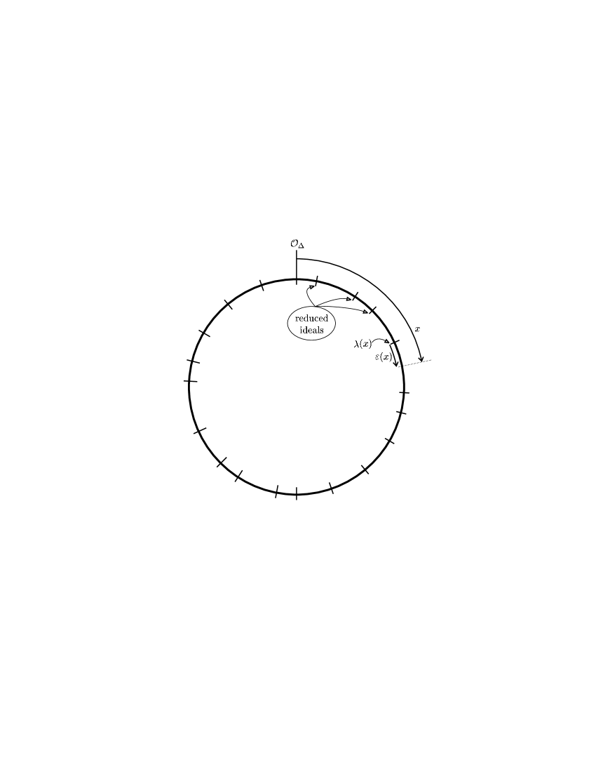
Figure 13.1: The Cycle Of Reduced Principal Ideals

It should be noted that the distances with which the participants in the protocol must work are all real numbers, and so to perform the required calculations exactly would require infinite precision. The participants must therefore choose some finite precision within which to perform all of the calculations, and as a result there may be round-off errors that propagate through the protocol. These potential round-off errors force the participants to perform an extra “clean-up” round of communication after the one usual round of a Diffie-Hellman-like exchange in order to make sure that they share the same value.

We can now sketch the protocol. There are many details of the implementation that are omitted in the presentation below; for a more complete description of the protocol, refer to [SBW94].

Algorithm 13.15 (Buchmann-Williams Protocol (Real Case)).

1. Alice and Bob agree on a discriminant $\Delta>0$, $\Delta\equiv 0,1\pmod{4}$ and an equivalence class of $Cl_{\Delta}$. (These choices can be made public.)

2. Alice chooses an integer $a$ uniformly at random from $\{1,\ldots,\lfloor\sqrt{\Delta}\,\rfloor\}$. She computes $\mathfrak{a}$, the ideal to the left of $a$; that is, $\mathfrak{a}=\mathop{\lambda}\!\left(a\right)$. She also computes $\mathop{\varepsilon}\!\left(a\right)$ and sends $\mathfrak{a}$ and $\mathop{\varepsilon}\!\left(a\right)$ to Bob.

3. Bob chooses an integer $b$ uniformly at random from $\{1,\ldots,\lfloor\sqrt{\Delta}\,\rfloor\}$. He computes $\mathfrak{b}$, the ideal to the left of $b$; that is, $\mathfrak{b}=\mathop{\lambda}\!\left(b\right)$. He also computes $\mathop{\varepsilon}\!\left(b\right)$ and sends $\mathfrak{b}$ and $\mathop{\varepsilon}\!\left(b\right)$ to Alice.

4. Alice computes $\mathfrak{c}_{A}$, the ideal to the left of $a+\mathop{\varepsilon}\!\left(b\right)$ (relative to $\mathfrak{b}$); that is, $\mathfrak{c}_{A}=\mathop{\lambda}\!\left(a+\mathop{\varepsilon}\!\left(b\right),\mathfrak{b}\right)$.

5. Bob computes $\mathfrak{c}_{B}$, the ideal to the left of $b+\mathop{\varepsilon}\!\left(a\right)$ (relative to $\mathfrak{a}$); that is, $\mathfrak{c}_{B}=\mathop{\lambda}\!\left(b+\mathop{\varepsilon}\!\left(a\right),\mathfrak{a}\right)$.

6. Alice and Bob send each other one classical bit which allows them to determine whether $\mathfrak{c}_{A}=\mathfrak{c}_{B}$. If this is not true, Alice and Bob make small adjustments (see [SBW94]) after which they are certain that they have computed the same ideal.

At the end of the protocol, Alice and Bob share a secret ideal which they can use to derive a secret key.

13.2 Security Of The Protocol

In this section we discuss the security of each of the two cases of the Buchmann-Williams protocol. As we will see, both cases are susceptible to attacks with a quantum computer. In order to break the real case of the protocol, however, we will need two recently discovered quantum algorithms.

13.2.1 The Imaginary Case

Since the imaginary case of the Buchmann-Williams protocol is equivalent to the Diffie-Hellman protocol, as mentioned in Chapter 12 the scheme would be broken if the Discrete Logarithm Problem (DLP) could be solved efficiently in the group $Cl_{\Delta}$. There are no known efficient classical algorithms to solve DLP in this group, however: the best known algorithms still require superpolynomial time, like that in [Jac99]. Furthermore, in [BW88] it is mentioned that if an efficient algorithm to solve DLP in $Cl_{\Delta}$ did exist, it could likely be used to factor $\Delta$.

The group could possibly admit attacks that did not depend on solving DLP but on solving the Diffie-Hellman Problem (DHP) directly, but again, there is some evidence described in [BW88] that these attacks could also lead to algorithms to factor $\Delta$. These facts suggest that breaking the scheme with a classical computer is at least as hard as the factoring problem, which we believe to be hard. We therefore believe the protocol to be secure against a passive adversary with a classical computer.

However, as mentioned in Section 3.8, there is an efficient quantum algorithm to solve DLP. In other words, this protocol is not secure against a quantum adversary.

13.2.2 The Real Case

Consider the following variation of DLP as proposed in [BW90]:

Problem 13.16 (Principal Ideal Distance Problem (PIDP)).

Given a principalideal $\mathfrak{a}$ of a real quadratic order $\mathcal{O}_{\Delta}$, compute $\mathop{\delta}\!\left(\mathfrak{a}\right)$, its distance from $\mathcal{O}_{\Delta}$.

Suppose an adversary can solve PIDP. When Alice sends $\mathfrak{a}$ and $\mathop{\varepsilon}\!\left(a\right)$ to Bob, the adversary can compute $\mathop{\delta}\!\left(\mathfrak{a}\right)$, and hence determine $\mathop{\delta}\!\left(\mathfrak{a}\right)+\mathop{\varepsilon}\!\left(a\right)=a$. The adversary then has knowledge of Alice’s private value $a$ (to some finite precision). With this knowledge, with good probability the adversary can construct the shared secret in the same way Alice does, and the protocol is broken. That is, an algorithm to solve PIDP would allow an adversary to break the real version of the Buchmann-Williams key establishment protocol.

There is evidence that PIDP is hard to solve with a classical computer. It is shown in [BW90] that an efficient solution to PIDP would result in an efficient algorithm to compute the regulator $R_{\Delta}$. Further, it is shown in [Sch82] that an efficient algorithm to compute $R_{\Delta}$ would result in an efficient algorithm to factor $\Delta$. Thus, PIDP is at least as hard as the factoring problem, which we believe to be hard with a classical computer. We therefore believe the protocol to be secure against a passive adversary with a classical computer.

However, as recently discovered by Hallgren [Hal02], we can efficiently solve PIDP with a quantum computer. Therefore the real version of the Buchmann-Williams key establishment protocol can be broken by a passive adversary with a quantum computer.

The remainder of this chapter introduces the new quantum algorithms that efficiently solve PIDP. Suppose we are given a quadratic order $\mathcal{O}_{\Delta}$. We will describe two algorithms: one that computes $R_{\Delta}$, and another that given $R_{\Delta}$ solves PIDP. The description of these algorithms in [Hal02] is quite terse, and the presentation below attempts to provide more details and to correct some of the minor errors in [Hal02]. A similar but independently constructed clarification of the algorithm to compute the regulator can be found in [Joz03], along with much of the background material already presented in this chapter.

13.2.3 Computing The Regulator

As mentioned above, much of the material in this section can also be found in [Joz03]. However, except where noted, the presentation here was developed independently.

We work in the identity class of $Cl_{\Delta}$. Consider the function $g\colon\mathbb{R}\longrightarrow\mathcal{P}_{\Delta}\!\times\mathbb{R}$ defined by $g(x)=\left(\mathop{\lambda}\!\left(x\right),\mathop{\varepsilon}\!\left(x\right)\right)$ for all $x\in\mathbb{R}$.

Proposition 13.17.

The function $g$ is one-to-one on the interval $[0,R_{\Delta})$ and periodic with period $R_{\Delta}$.

Proof.

If $g(x)=g(y)$ for any $x,y\in[0,R_{\Delta})$, then $\mathop{\lambda}\!\left(x\right)=\mathop{\lambda}\!\left(y\right)$ and

$$\mathop{\varepsilon}\!\left(x\right) =\mathop{\varepsilon}\!\left(y\right)$$

$$x-\mathop{\delta}\!\left(\mathop{\lambda}\!\left(x\right)\right) \equiv y-\mathop{\delta}\!\left(\mathop{\lambda}\!\left(y\right)\right)\pmod{R_{\Delta}}$$

$$x-\mathop{\delta}\!\left(\mathop{\lambda}\!\left(x\right)\right) \equiv y-\mathop{\delta}\!\left(\mathop{\lambda}\!\left(x\right)\right)\pmod{R_{\Delta}}$$

$$x \equiv y\pmod{R_{\Delta}}.$$

Further, $x,y\in[0,R_{\Delta})$ so it follows that $x=y$, and $g$ is one-to-one on $[0,R_{\Delta})$.

Since the distance around the cycle of reduced ideals is $R_{\Delta}$, it follows that for any $x\in\mathbb{R}$,

$$g(x+R_{\Delta}) =\left(\mathop{\lambda}\!\left(x+R_{\Delta}\right),\mathop{\varepsilon}\!\left(x+R_{\Delta}\right)\right)$$

$$=\left(\mathop{\lambda}\!\left(x\right),\mathop{\varepsilon}\!\left(x\right)\right)$$

$$=g(x)$$

so $g$ is periodic with period $R_{\Delta}$. ∎

We now have a periodic function with a domain of $\mathbb{R}$. We would like to use techniques similar to those from Section 3.4 to find the period of the function, but in order to compute with the function we first have to modify it slightly so that its domain is some discrete set. Such a modification will also have the effect of making the function no longer “perfectly” periodic, but we will still be able to recover a close approximation to the period.

More specifically, as in [Hal02] we can define what it means for a function with an integer domain to be “periodic” with a real (not necessarily integer) period. We use the definition presented in [Joz03]:

Definition 13.18.

Let $X$ be any set. A function $f\colon\mathbb{Z}\longrightarrow X$ is called weakly periodic with period $s\in\mathbb{R}$ if for all integers $k$, $0\leq k<s$, and for all non-negative integers $j$, either

1. $f(k)=f(k+\lfloor js\rfloor)$, or

2. $f(k)=f(k+\lceil js\rceil)$.

For brevity we will write $f(k)=f(k+\left[js\right])$ to indicate that one of the above conditions is satisfied. The satisfied condition may vary with $k$ and $j$.

(Here we use the notation $\left\lfloor x\right\rfloor$ to denote the largest integer less than or equal to $x$, and $\left\lceil x\right\rceil$ to denote the smallest integer greater than or equal to $x$. We will also use the notation $\left\lfloor x\right\rceil$ to denote the closest integer to $x$.)

We now define a weakly periodic function by slightly modifying the function $g$. Given a positive integer $N$, we define $\hat{g}\colon\mathbb{Z}\longrightarrow\mathcal{P}_{\Delta}\!\times\mathbb{Z}$ by $\hat{g}(j)=\left(\mathop{\lambda}\!\left(\tfrac{j}{N}\right),\left\lfloor N\mathop{\varepsilon}\!\left(\tfrac{j}{N}\right)\right\rfloor\right)$ for all integers $j$.

As we will see, this function does not precisely satisfy the definition of a weakly periodic function, but by choosing $N$ wisely we can ensure that it satisfies the definition for a large fraction of the integers $k$, $0\leq k<s$. This statement is made more specific in the following theorem:

Theorem 13.19.

If $N\geq n\frac{32\Delta}{3}$ then the function $\hat{g}$ is one-to-one on the interval $[0,NR_{\Delta})$ and $\hat{g}(k)=\hat{g}(k+\left[jNR_{\Delta}\right])$ for at least a $\left(1-\frac{1}{O\!\left(n\right)}\right)$ fraction of the integers $k\in[0,NR_{\Delta})$.

Note that in the analogous theorem in [Hal02], it is stated without proof that we should require only $N\geq n\sqrt{\Delta}$. However, precise analysis in [Joz03] proves the existence of the lower bound on $N$ given in Theorem 13.19; so we use that lower bound here.

Proof.

First we show that $\hat{g}$ is one-to-one on the interval $[0,NR_{\Delta})$.

If $\hat{g}(j)=\hat{g}(k)$ for any $j,k\in[0,NR_{\Delta})$ then $\mathop{\lambda}\!\left(\frac{j}{N}\right)=\mathop{\lambda}\!\left(\frac{k}{N}\right)$ and

$$\lfloor N\mathop{\varepsilon}\!\left(\tfrac{j}{N}\right)\rfloor =\left\lfloor N\mathop{\varepsilon}\!\left(\tfrac{k}{N}\right)\right\rfloor$$

$$N\mathop{\varepsilon}\!\left(\tfrac{j}{N}\right) =N\mathop{\varepsilon}\!\left(\tfrac{k}{N}\right)+\sigma$$

for some $\sigma$ with $\left|\sigma\right|<1$. Dividing both sides by $N$, we get

$$\mathop{\varepsilon}\!\left(\tfrac{j}{N}\right) =\mathop{\varepsilon}\!\left(\tfrac{k}{N}\right)+\tfrac{\sigma}{N}$$

$$\tfrac{j}{N}-\mathop{\delta}\!\left(\mathop{\lambda}\!\left(\tfrac{j}{N}\right)\right) \equiv\tfrac{k}{N}-\mathop{\delta}\!\left(\mathop{\lambda}\!\left(\tfrac{k}{N}\right)\right)+\tfrac{\sigma}{N}\pmod{R_{\Delta}}$$

$$\tfrac{j}{N}-\mathop{\delta}\!\left(\mathop{\lambda}\!\left(\tfrac{j}{N}\right)\right) \equiv\tfrac{k}{N}-\mathop{\delta}\!\left(\mathop{\lambda}\!\left(\tfrac{j}{N}\right)\right)+\tfrac{\sigma}{N}\pmod{R_{\Delta}}$$

$$\tfrac{j}{N} \equiv\tfrac{k}{N}+\tfrac{\sigma}{N}\pmod{R_{\Delta}}.$$

Since $0\leq j,k<NR_{\Delta}$, we must have $0\leq\frac{j}{N},\frac{k}{N}<R_{\Delta}$. Therefore, $\frac{j}{N}=\frac{k}{N}+\frac{\sigma}{N}$. Further, since $j,k\in\mathbb{Z}$ and $\left|\sigma\right|<1$, we must in fact have $\sigma=0$, so $j=k$ and thus $\hat{g}$ is one-to-one on $[0,NR_{\Delta})$.

Now we wish to show that $\hat{g}(k)=\hat{g}(k+\left[jNR_{\Delta}\right])$ for a sufficiently large fraction of the integers $k\in[0,NR_{\Delta})$. Choose any reduced ideal $\mathfrak{a}$, and consider the interval between the distance of $\mathfrak{a}$ and the distance of the next ideal in the cycle; in other words, the interval $I=\left[\mathop{\delta}\!\left(\mathfrak{a}\right),\mathop{\delta}\!\left(\rho(\mathfrak{a})\right)\right)$. By a proven bound on the distance between consecutive ideals developed in [Joz03] we know that $I$ has length at least $\frac{3}{32\Delta}$.

Since we are given $N\geq n\frac{32\Delta}{3}$, we know that $\frac{3}{32\Delta}\geq\frac{n}{N}$, and hence there are at least $n$ integers $k$ in $[0,NR_{\Delta})$ for which $\frac{k}{N}\in I$. Let $S$ be the set of all such integers.

For any $k\in S$, $\mathop{\lambda}\!\left(\frac{k}{N}\right)=\mathfrak{a}$. Further, if $k\neq\min S$ and $k\neq\max S$, and $\sigma$ is chosen such that $0\leq\sigma<1$, then $\max S<k\pm\sigma<\min S$, so

$$\mathop{\lambda}\!\left(\tfrac{k\pm\sigma}{N}\right)=\mathop{\lambda}\!\left(\tfrac{k}{N}\right)=\mathfrak{a}.$$ (13.1)

Fix some value of $j$, and define the quantity $\sigma_{1}=jNR_{\Delta}-\left\lfloor jNR_{\Delta}\right\rfloor$. We assume that $jNR_{\Delta}\not\in\mathbb{Z}$, so $0<\sigma_{1}<1$.

We consider two cases:

1. If we round down the value of $jNR_{\Delta}$,

   $$\mathop{\lambda}\!\left(\tfrac{k+\left\lfloor jNR_{\Delta}\right\rfloor}{N}\right) =\mathop{\lambda}\!\left(\tfrac{k+jNR_{\Delta}-\sigma_{1}}{N}\right)$$

   $$=\mathop{\lambda}\!\left(\tfrac{k-\sigma_{1}}{N}+jR_{\Delta}\right)$$

   $$=\mathop{\lambda}\!\left(\tfrac{k-\sigma_{1}}{N}\right)$$

   $$=\mathop{\lambda}\!\left(\tfrac{k}{N}\right)\quad\mbox{by~{}Equation~{}\eqref{equ:BW:leftIdealRounding}.}$$

2. Similarly, if we round up the value of $jNR_{\Delta}$,

   $$\mathop{\lambda}\!\left(\tfrac{k+\left\lceil jNR_{\Delta}\right\rceil}{N}\right) =\mathop{\lambda}\!\left(\tfrac{k+jNR_{\Delta}+(1-\sigma_{1})}{N}\right)$$

   $$=\mathop{\lambda}\!\left(\tfrac{k+(1-\sigma_{1})}{N}\right)$$

   $$=\mathop{\lambda}\!\left(\tfrac{k}{N}\right)\quad\mbox{by~{}Equation~{}\eqref{equ:BW:leftIdealRounding}.}$$

Thus for any $k\in S$, $k\neq\min S$, $k\neq\max S$,

$$\mathop{\lambda}\!\left(\tfrac{k+\left\lfloor jNR_{\Delta}\right\rfloor}{N}\right)=\mathop{\lambda}\!\left(\tfrac{k}{N}\right)=\mathop{\lambda}\!\left(\tfrac{k+\left\lceil jNR_{\Delta}\right\rceil}{N}\right).$$ (13.2)

Now define the quantity $\sigma_{2}=N\mathop{\varepsilon}\!\left(\frac{k}{N}\right)-\left\lfloor N\mathop{\varepsilon}\!\left(\frac{k}{N}\right)\right\rfloor$. Then $0\leq\sigma_{2}<1$.

Again, we consider two cases:

1. If $\sigma_{1}\leq\sigma_{2}$, then

   $$\left\lfloor N\mathop{\varepsilon}\!\left(\tfrac{k+\left\lfloor jNR_{\Delta}\right\rfloor}{N}\right)\right\rfloor =\left\lfloor N\mathop{\varepsilon}\!\left(\tfrac{k-\sigma_{1}}{N}+jR_{\Delta}\right)\right\rfloor$$

   $$=\left\lfloor N\left(\tfrac{k-\sigma_{1}}{N}-\mathop{\delta}\!\left(\mathop{\lambda}\!\left(\tfrac{k-\sigma_{1}}{N}\right)\right)\right)\right\rfloor$$

   $$=\left\lfloor N\left(\tfrac{k}{N}-\tfrac{\sigma_{1}}{N}-\mathop{\delta}\!\left(\mathop{\lambda}\!\left(\tfrac{k}{N}\right)\right)\right)\right\rfloor$$

   $$=\left\lfloor N\mathop{\varepsilon}\!\left(\tfrac{k}{N}\right)-\sigma_{1}\right\rfloor$$

   $$=\left\lfloor N\mathop{\varepsilon}\!\left(\tfrac{k}{N}\right)\right\rfloor\quad\mbox{since $\sigma_{1}\leq\sigma_{2}$.}$$

2. If $\sigma_{1}>\sigma_{2}$, then similarly

   $$\left\lfloor N\mathop{\varepsilon}\!\left(\tfrac{k+\left\lceil jNR_{\Delta}\right\rceil}{N}\right)\right\rfloor =\left\lfloor N\mathop{\varepsilon}\!\left(\tfrac{k+(1-\sigma_{1})}{N}+jR_{\Delta}\right)\right\rfloor$$

   $$=\left\lfloor N\mathop{\varepsilon}\!\left(\tfrac{k}{N}\right)+(1-\sigma_{1})\right\rfloor$$

   $$=\left\lfloor N\mathop{\varepsilon}\!\left(\tfrac{k}{N}\right)\right\rfloor\quad\mbox{since $1-\sigma_{1}<1-\sigma_{2}$.}$$

Thus for any $k\in S$ with $k\neq\min S$, $k\neq\max S$,

$$\left\lfloor N\mathop{\varepsilon}\!\left(\tfrac{k+\left[jNR_{\Delta}\right]}{N}\right)\right\rfloor=\left\lfloor N\mathop{\varepsilon}\!\left(\tfrac{k}{N}\right)\right\rfloor.$$ (13.3)

Combining Equation (13.2) and Equation (13.3), we see that

$$\hat{g}(k+\left[jNR_{\Delta}\right])=\hat{g}(k).$$ (13.4)

Since $\left|S\right|\geq n$ and $k$ can take on all but two of the values in $S$, Equation (13.4) is satisfied for at least a $\left(1-\frac{2}{n}\right)$ fraction of the integers $k\in S$. The same argument can be made for the interval between any two reduced ideals. Thus Equation (13.4) is satisfied for at least a $\left(1-\frac{2}{n}\right)$ fraction of the integers $k\in[0,NR_{\Delta})$. (This bound can in fact be improved to a $\left(1-\frac{1}{n}\right)$ fraction with a slightly different analysis like that of [Joz03], but the bound presented here is still sufficient.)

Therefore as required, $\hat{g}(k+\left[jNR_{\Delta}\right])=\hat{g}(k)$ for at least a $\left(1-\frac{1}{O\!\left(n\right)}\right)$ fraction of the integers $k\in[0,NR_{\Delta})$. ∎

We can now describe the core of the quantum algorithm to compute the regulator. The algorithm will calculate an approximation to $s=NR_{\Delta}$, from which we can recover $R_{\Delta}$. Like in Algorithm 3.11, we assume that we have a unitary operator $\textup{{U}}_{\hat{g}}$ that maps $\left|x\right>\left|y\right>\longmapsto\left|x\right>\left|y\oplus\hat{g}(x)\right>$. We also assume that we are given an integer $m>3s^{3}$, although if the approximate size of $s$ is unknown, we can use a technique similar to that of Section 3.4, where we repeatedly double $m$ until the algorithm succeeds.

Algorithm 13.20 (Core Of Computing The Regulator).

1. Start in the state $\left|0\right>\left|0\right>\in\mathbb{H}_{m}\otimes\mathbb{H}_{l}$, where $l$ is chosen such that $l$ bits are sufficient to encode any point in the range of $\hat{g}$.

2. Apply $\textup{{QFT}}_{m}$ to the first register.

3. Apply $\textup{{U}}_{\hat{g}}$ to the system.

4. Measure the second register.

5. Apply $\textup{{QFT}}_{m}$ to the first register.

6. Measure the first register to obtain the integer $y$. If $y>\frac{m}{n}$, begin the procedure again.

7. Otherwise, return $y$.

Theorem 13.21.

With probability in $O\!\left(\frac{1}{\log{s}}\right)$, the output of Algorithm 13.20 satisfies $y=\left\lfloor k\frac{m}{s}\right\rceil$ for some integer $k$.

Proof Sketch.

After Step 3 our system is in the state $\left|\phi\right>=\frac{1}{\sqrt{m}}\sum_{x=0}^{m-1}\left|x\right>\left|\hat{g}(x)\right>$. When we measure the second register in Step 4, we see a value $z$, and we leave the first register in a superposition of all states in which $z$ appears in the second register.

We now determine this superposition. Let $m=\left\lfloor ps\right\rfloor+r$ where $p,r\in\mathbb{Z}$ and $0<r\leq s$; in other words, $m\approx ps$. By Theorem 13.19 we know that for an inverse polynomial fraction of the integers $k$ with $0\leq k<s$, $\hat{g}(k)=\hat{g}(k+\left[js\right])$. So with high probability, if $z=\hat{g}(k)$, then $z=\hat{g}(k+\left[js\right])$ for all $j$, $0\leq j<p$. Thus we can say that after Step 4 we leave the first register in a state that is “close to”

$$\left|\psi\right>=\frac{1}{\sqrt{p}}\sum_{j=0}^{p-1}\left|k+\left[js\right]\right>.$$

This is not exactly the state of the first register, since the function $\hat{g}$ is not exactly weakly periodic. The consequences of using this approximate data are not explicitly analysed in [Hal02] or [Joz03]. However, both claim that because of the large fraction of integers $k$ for which $\hat{g}(k)=\hat{g}(k+\left[js\right])$ (see Theorem 13.19) the approximation is close enough for the algorithm to succeed. Similarly, the remainder of the analysis here assumes that the first register is in the exact state $\left|\psi\right>$.

After applying $\textup{{QFT}}_{m}$ to $\left|\psi\right>$ in Step 5, we obtain the state

$$\frac{1}{\sqrt{pm}}\sum_{j=0}^{p-1}\sum_{x=0}^{m-1}e^{2\pi ix\frac{k+\left[js\right]}{m}}\left|x\right>$$

$$=e^{2\pi i\frac{k}{m}}\frac{1}{\sqrt{pm}}\sum_{x=0}^{m-1}\sum_{j=0}^{p-1}e^{2\pi ix\frac{\left[js\right]}{m}}\left|x\right>.$$

It is interesting to note that the global phase coefficient $e^{2\pi i\frac{k}{m}}$ does not affect the probability distribution of the results of measuring this state, since $\left|e^{2\pi i\frac{k}{m}}\right|^{2}=1$. (In other words, we can assume without loss of generality that $k=0$. It is a general property of the Fourier sampling method used by this algorithm that given a group $G$ and a subset $X$ of $G$, the distributions induced by applying the method to the superpositions $\sum_{x\in X}\left|x\right>$ and $\sum_{x\in X}\left|g+x\right>$ are identical for every $g\in G$ [Hal02].)

The probability of obtaining a particular measurement result $y$ in Step 6 is therefore given by

$$P_{y}=\left|\frac{1}{\sqrt{pm}}\sum_{j=0}^{p-1}e^{2\pi iy\frac{\left[js\right]}{m}}\right|^{2}.$$ (13.5)

As in [Hal02] (but in more detail) we now analyse this distribution.

Fix a value $y=\left\lfloor k\frac{m}{s}\right\rceil$ for some integer $k$, and let $y=k\frac{m}{s}+\varepsilon$ where $-\frac{1}{2}\leq\varepsilon<\frac{1}{2}$. For each $j$, $0\leq j<p$, let $\left[js\right]=js+\delta_{j}$, where $-1\leq\delta_{j}<1$.

Then note that

$$y\frac{\left[js\right]}{m} =\left(\frac{k}{s}+\frac{\varepsilon}{m}\right)\left(js+\delta_{j}\right)$$

$$=kj+\frac{\varepsilon js}{m}+\frac{k\delta_{j}}{s}+\frac{\varepsilon\delta_{j}}{m}.$$ (13.6)

Recall that in Step 6 we accepted only values of $y$ that satisfied $y\leq\frac{m}{n}$. Thus

$$\frac{km}{s}+\varepsilon \leq\frac{m}{n}$$

$$\frac{k}{s}+\frac{\varepsilon}{m} \leq\frac{1}{n}$$

$$\left|\frac{k\delta_{j}}{s}+\frac{\varepsilon\delta_{j}}{m}\right| \leq\left|\frac{\delta_{j}}{n}\right|$$

$$\left|\frac{k\delta_{j}}{s}+\frac{\varepsilon\delta_{j}}{m}\right| <\frac{1}{n}.$$ (13.7)

Further note that $\frac{\varepsilon js}{m}=\left(\frac{j}{p}\right)\left(\frac{\varepsilon sp}{m}\right)$ and

$$\left|\frac{\varepsilon sp}{m}\right|\approx\left|\frac{\varepsilon sp}{sp}\right|\leq\frac{1}{2}.$$ (13.8)

We now appeal to Claim 3.2 of [Hal02], which we re-state more precisely but do not prove. (See [Joz03] for a proof of the claim’s correctness.) The claim is the following:

Proposition 13.22.

Let $n$ and $q$ be positive integers, let $\alpha$ be a constant, $\left|\alpha\right|\leq\frac{3}{4}$, and let $\beta\colon\mathbb{Z}\rightarrow\mathbb{R}$ be a function such that $\left|\beta(j)\right|\leq\frac{1}{n}$ for all $j$, $0\leq j<q-1$. Then there exists a constant $c$ such that if $n\in O\!\left(\log q\right)$,

$$\left|\sum_{j=0}^{q-1}e^{2\pi i\left(\frac{j}{q}\alpha+\beta(j)\right)}\right|^{2}\geq cq^{2}.$$

If we let $\beta(j)=\frac{k\delta_{j}}{s}+\frac{\varepsilon\delta_{j}}{m}$ and $\alpha=\frac{\varepsilon sp}{m}$, then by Equation (13.7) and Equation (13.8), respectively, the hypotheses of Proposition 13.22 are satisfied.

Further, combining Equation (13.5) and Equation (13.6), we see that

$$P_{y} =\left|\frac{1}{\sqrt{pm}}\sum_{j=0}^{p-1}\exp\left(2\pi i\left(kj+\frac{\varepsilon js}{m}+\frac{k\delta_{j}}{s}+\frac{\varepsilon\delta_{j}}{m}\right)\right)\right|^{2}$$

$$=\frac{1}{pm}\left|\sum_{j=0}^{p-1}\exp\left(2\pi i\left(\frac{\varepsilon js}{m}+\frac{k\delta_{j}}{s}+\frac{\varepsilon\delta_{j}}{m}\right)\right)\right|^{2}$$

$$=\frac{1}{pm}\left|\sum_{j=0}^{p-1}e^{2\pi i\left(\left(\frac{j}{p}\right)\alpha+\beta(j)\right)}\right|^{2}.$$

We can therefore apply Proposition 13.22 to the above sum, and deduce that

$$P_{y}\geq\frac{1}{pm}cp^{2}\approx\frac{c}{s}.$$

Finally, we calculate the number of $y$ that satisfy the conditions of the theorem. By the condition in Step 6 we know that $0\leq y\leq\frac{m}{n}$. Using the fact that $\log{s}>n$, we can obtain a lower bound on the number of such $y$ by counting only those that satisfy

$$0\leq y\leq\frac{m}{\log{s}}.$$ (13.9)

If $0\leq\left\lfloor k\frac{m}{s}\right\rceil\leq\frac{m}{\log{s}}$, then $0\leq k\leq\frac{s}{\log{s}}$ (approximately); so there are $\frac{s}{\log{s}}$ values of $y$ that satisfy the conditions of the theorem and Equation (13.9).

The probability that the output of the algorithm satisfies the conditions of the theorem is therefore at least

$$\frac{s}{\log{s}}\cdot P_{y} =\frac{s}{\log{s}}\cdot\frac{c}{s}$$

$$=\frac{c}{\log{s}}$$

which is in $O\!\left(\frac{1}{\log{s}}\right)$ as required. ∎

The basic statement of Theorem 13.21 is that the probability of measuring such an integer $y$ is considerably higher than selecting the integer $y$ uniformly at random from $0,\ldots,m-1$.

The remainder of the algorithm to compute the regulator is purely classical and similar to Algorithm 3.11 to solve the bounded case of the Integer Hidden Subgroup Problem (IHSP); we do not prove its correctness here (see [Hal02] or [Joz03]). The algorithm works as follows: we run Algorithm 13.20 twice, obtaining integers $y_{1}$ and $y_{2}$ which by Theorem 13.21 with high probability are equal to $\left\lfloor k_{1}\frac{m}{s}\right\rceil$ and $\left\lfloor k_{2}\frac{m}{s}\right\rceil$ for some integers $k_{1}$ and $k_{2}$. Also, with high probability, $\gcd(k_{1},k_{2})=1$. Applying the continued fraction algorithm from Section 3.4 to $\frac{y_{1}}{y_{2}}$, and using an algorithm from [Hal02] to test whether a given integer is “close to” a multiple of $s$, we can recover the integer $k_{1}$.

Once we have recovered $k_{1}$, we can compute

$$a =\left\lfloor\frac{k_{1}m}{y_{1}}\right\rceil$$

$$=\left\lfloor\frac{k_{1}m}{k_{1}\frac{m}{s}}\right\rceil$$

$$=\left\lfloor s\right\rceil.$$

The final step of the algorithm is to compute $\frac{a}{N}$; note that

$$\left|a-s\right| <1$$

$$\left|a-NR_{\Delta}\right| <1$$

$$\left|\frac{a}{N}-R_{\Delta}\right| <\frac{1}{N}$$

In other words, this polynomial time quantum algorithm allows us to determine the regulator to arbitrary precision depending on our choice of $N$.

13.2.4 Solving The Principal Ideal Distance Problem

After computing the regulator, we can use another new quantum algorithm from [Hal02] to solve PIDP. Given an ideal $\mathfrak{a}$, let the (unknown) distance of $\mathfrak{a}$ be $a$. The goal of the algorithm is to find $a$. We will use an algorithm similar to the algorithm in Section 3.8 for solving the Discrete Logarithm Problem (DLP).

We begin by defining a new periodic function, as suggested in [Zal03], that is based on the function $g$ from the previous section, although this new function has a two-dimensional domain. Consider the function $h\colon\mathbb{Z}\times\mathbb{R}\longrightarrow\mathcal{P}_{\Delta}\times\mathbb{R}$ defined by

$$h(j,x) =g(aj+x)$$

$$=\left(\mathop{\lambda}\!\left(aj+x\right),\mathop{\varepsilon}\!\left(aj+x\right)\right).$$

We briefly justify that this function is periodic with a two-dimensional period given by $p_{1}=(0,R_{\Delta})$ and $p_{2}=(-1,a)$:

1. Note that $h((j,x)+p_{1})=h(j,x+R_{\Delta})=g(aj+x+R_{\Delta})=g(aj+x)$ since $g$ is periodic with period $R_{\Delta}$ by Proposition 13.17.

2. Note that $h((j,x)+p_{2})=h(j-1,x+a)=g(a(j-1)+x+a)=g(aj+x)$.

Thus $h$ is indeed a periodic function with the given two dimensional period. Note that the unknown value $a$ appears in $p_{2}$, so if we could find the period of this function, we could solve PIDP.

As in the previous section, we cannot easily compute with $h$, since the domain is not a discrete set. We therefore modify $h$ slightly, and define a new function $\hat{h}\colon\mathbb{Z}\times\mathbb{Z}\rightarrow\mathcal{P}_{\Delta}\times\mathbb{Z}$ by

$$\hat{h}(j_{1},j_{2})=\left(\mathop{\lambda}\!\left(aj_{1}+\frac{j_{2}}{N}\right),\left\lfloor N\mathop{\varepsilon}\!\left(aj_{1}+\frac{j_{2}}{N}\right)\right\rfloor\right).$$

(Note that $\hat{h}(j_{1},j_{2})=\hat{g}\left(aj_{1}+\frac{j_{2}}{N}\right)$ where the domain of $\hat{g}$ has been extended to $\mathbb{R}$ in the natural way.) This function $\hat{h}$ is the function proposed in [Hal02] and it is the function on which the solution to PIDP is based.

At first it seems as though we cannot evaluate $\hat{h}$ since we do not know $a$. However, using an algorithm described in detail in [SBW94], given $\mathfrak{a}$ we can compute the ideal to the left of $\mathop{\delta}\!\left(\mathfrak{a}\right)j_{1}$ and its error; that is, we can compute $\mathop{\lambda}\!\left(aj_{1}\right)$ and $\mathop{\varepsilon}\!\left(aj_{1}\right)$. Since the value $\frac{j_{2}}{N}$ is known, we can use the methods described in Section 13.1.2 (in fact the same methods that Alice and Bob use to carry out the real Buchmann-Williams protocol) to compute $\mathop{\lambda}\!\left(aj_{1}+\frac{j_{2}}{N}\right)$ and $\mathop{\varepsilon}\!\left(aj_{1}+\frac{j_{2}}{N}\right)$. (Note that at the end of these computations we still do not know the value of $a$.)

We will solve a problem similar to the Hidden Subgroup Problem (HSP), although in this case we do not have a hidden subgroup, but instead a hidden “group-like set”. Consider the set $T=\left\{(s,t)\in\mathbb{Z}\times\mathbb{Z}\,:\,\left(as+\tfrac{t}{N}\right)\bmod{R_{\Delta}}<\tfrac{1}{N}\right\}$. The function $\hat{h}$ is constant on $T$ because the interval $\left[0,\frac{1}{N}\right)$ is short enough that it contains only the ideal $\mathcal{O}_{\Delta}$, and thus for any $x$ in the interval $\mathop{\lambda}\!\left(x\right)=\mathcal{O}_{\Delta}$ and $\left\lfloor N\mathop{\varepsilon}\!\left(x\right)\right\rfloor=0$. So for any $(s,t)\in T$, $\hat{h}(s,t)=(\mathcal{O}_{\Delta},0)$.

Next consider a coset of $T$, say $T+(u,v)$. We can write this coset as follows:

$$T+(u,v) =\left\{(s,t)\in\mathbb{Z}\times\mathbb{Z}\,:\,\left(a(s-u)+\tfrac{t-v}{N}\right)\bmod{R_{\Delta}}<\tfrac{1}{N}\right\}$$

$$=\left\{(s,t)\in\mathbb{Z}\times\mathbb{Z}\,:\,\left(as+\tfrac{t}{N}-\left(us+\tfrac{v}{N}\right)\right)\bmod{R_{\Delta}}<\tfrac{1}{N}\right\}.$$

In other words, this coset of $T$ is the set of points $(s,t)$ such that $as+\frac{t}{N}$ is in the interval of length $\frac{1}{N}$ starting from $us+\tfrac{v}{N}$. We will denote this interval by $I_{(u,v)}$.

Unlike in an instance of the typical HSP, the function $h$ is not necessarily constant on the cosets of $T$. For example, suppose there is an ideal $\mathfrak{b}$ in the interval $I_{(u,v)}$. Then for the points $x\in I_{(u,v)}$ after $\mathfrak{b}$, $\mathop{\lambda}\!\left(x\right)=\mathfrak{b}$, but for the rest of the points $x$, $\mathop{\lambda}\!\left(x\right)=\rho^{-1}(\mathfrak{b})$ (the previous ideal in the cyclical ordering). Similarly, if there is a point $y\in I_{(u,v)}$ such that the distance from $y$ to $\mathop{\lambda}\!\left(y\right)$ is a multiple of $\frac{1}{N}$ then the value of $\left\lfloor N\mathop{\varepsilon}\!\left(x\right)\right\rfloor$ will change depending on whether $x$ occurs before or after $y$.

It is in fact true that $\hat{h}$ could take on at most $3$ values on any coset of $T$, in the case where the corresponding interval contains both an ideal $\mathfrak{b}$ and a value $y$ such that the distance from $y$ to $\mathop{\lambda}\!\left(y\right)$ is a multiple of $\frac{1}{N}$. Consequently, $\hat{h}$ must be constant on at least $\frac{1}{3}$ of the elements in the coset. Although the implications of $\hat{h}$ being only “approximately constant” on the cosets of $T$ are not explicitly analysed in [Hal02], the fraction of the elements on which $\hat{h}$ is constant is sufficient to allow the algorithm to succeed.

It should also be noted that two cosets of $T$ may overlap without being exactly equal, since we could have $au+\frac{v}{N}\approx au^{\prime}+\frac{v^{\prime}}{N}$ with $v\neq v^{\prime}$ and $u\neq u^{\prime}$. However, for fixed $u$ and $0\leq v<NR_{\Delta}$ it is true that the cosets $\left\{T+(u,v)\right\}$ are disjoint, and $h$ is distinct and approximately constant on these disjoint cosets.

First we select the parameters for the algorithm using the following algorithm:

Algorithm 13.23 (Parameter Selection For PIDP).

1. Compute the regulator $R_{\Delta}$ using the algorithm from Section 13.2.3.

2. Choose an integer $m>2R_{\Delta}$.

3. Choose an integer $b>n\frac{32\Delta}{3}$ and compute the continued fraction expansion of $bR_{\Delta}$ to find $p,q\in\mathbb{Z}$ such that $\left|bR_{\Delta}-\frac{p}{q}\right|\leq\frac{1}{4qm}$.

4. Let $N=qb$.

5. Output $(R_{\Delta},m,N)$.

Proposition 13.24.

The output of Algorithm 13.23 satisfies $\left|NR_{\Delta}-\left\lfloor NR_{\Delta}\right\rceil\right|\leq\frac{1}{4m}$.

Proof.

We know that

$$\left|bR_{\Delta}-\frac{p}{q}\right| \leq\frac{1}{4qm}$$

$$\left|\frac{N}{q}R_{\Delta}-\frac{p}{q}\right| \leq\frac{1}{4qm}$$

$$\left|NR_{\Delta}-p\right| \leq\frac{1}{4m}.$$

Now since $p$ is an integer and its distance from $NR_{\Delta}$ is less than $\tfrac{1}{2}$, we must have $p=\left\lfloor NR_{\Delta}\right\rceil$. Thus

$$\left|NR_{\Delta}-\left\lfloor NR_{\Delta}\right\rceil\right| \leq\frac{1}{4m}$$

as required. ∎

Once the parameters have been selected, we can run the following algorithm to solve PIDP.

Algorithm 13.25 (Core Of Solving PIDP).

1. Start in the state $\left|0\right>\left|0\right>\left|0\right>\in\mathbb{H}_{mp}\otimes\mathbb{H}_{p}\otimes\mathbb{H}_{l}$, where $p=\left\lfloor NR_{\Delta}\right\rceil$ and $l$ is chosen such that $l$ bits are sufficient to encode any point in the range of $\hat{h}$.

2. Apply $\textup{{QFT}}_{mp}\otimes\textup{{QFT}}_{p}$ to the first two registers.

3. Apply $\textup{{U}}_{\hat{h}}$ to the system.

4. Measure the third register.

5. Apply $\textup{{QFT}}_{mp}\otimes\textup{{QFT}}_{p}$ to the first two registers.

6. Measure the first two registers to obtain the integers $(s,t)$. If $t>\frac{p}{n}$, begin the procedure again.

7. Otherwise, return $(s,t)$.

Theorem 13.26.

With probability in $O\!\left(\frac{1}{\log{\left(NR_{\Delta}\right)}}\right)$ the output $(s,t)$ of Algorithm 13.25 satisfies

$$\frac{s-\gamma_{t}}{mN}\equiv at\bmod{R_{\Delta}}$$

for some $\gamma_{t}$ with $\left|\gamma_{t}\right|\leq\frac{1}{2}$.

Proof Sketch.

First we claim that for any integer $s$, there is exactly one integer $t$ with $0\leq t<NR_{\Delta}$ such that $(s,t)\in T$. To see this, suppose that $(s,t_{1}),(s,t_{2})\in T$, with $0\leq t_{1},t_{2}<NR_{\Delta}$. Let $\varepsilon_{i}=\left(as+\frac{t_{i}}{N}\right)\bmod{R_{\Delta}}$ for $i=1,2$, and define the integers $k_{1}$ and $k_{2}$ such that $as+\frac{t_{i}}{N}=\varepsilon_{i}+k_{i}R_{\Delta}$. Then $0\leq\varepsilon_{1},\varepsilon_{2}<\frac{1}{N}$, so

$$\left|\varepsilon_{1}-\varepsilon_{2}\right| <\tfrac{1}{N}$$

$$\left|as+\tfrac{t_{1}}{N}-k_{1}R_{\Delta}-as-\tfrac{t_{2}}{N}+k_{2}R_{\Delta}\right| <\tfrac{1}{N}$$

$$\left|\tfrac{t_{1}-t_{2}}{N}+(k_{2}-k_{1})R_{\Delta}\right| <\tfrac{1}{N}$$

$$\left|\tfrac{t_{1}-t_{2}}{N}\right|\bmod{R_{\Delta}} <\tfrac{1}{N}$$

$$\left|t_{1}-t_{2}\right|\bmod{NR_{\Delta}} <1$$

Thus since $0\leq t_{1},t_{2}<NR_{\Delta}$ we must have $t_{1}=t_{2}$.

We now define

$$\hat{T}=\left\{(s,t)\in\mathbb{Z}\times\mathbb{Z}\,:\,0\leq t<NR_{\Delta},\left(as+\tfrac{t}{N}\right)\bmod{R_{\Delta}}<\frac{1}{N}\right\}$$

and it follows that for each $s\in\mathbb{Z}$, there is a unique element $(s,t)\in\hat{T}$.

For each $s\in\mathbb{Z}$, we can use this unique element $(s,t)$ to define $\sigma_{s}$ such that $\left(as-\frac{t}{N}\right)\bmod{R_{\Delta}}=\frac{\sigma_{s}}{N}.$ By the definition of $\hat{T}$, $0\leq\sigma_{s}<1$.

Then note that for each $(s,t)\in\hat{T}$,

$$as+\frac{t}{N}-\frac{\sigma_{s}}{N}=kR_{\Delta}$$ (13.10)

for some integer $k$.

Now note the following:

1. $t<NR_{\Delta}$, so $kR_{\Delta}<as+R_{\Delta}$, and

2. $\sigma_{s}<1$, so $as-\frac{1}{N}<kR_{\Delta}$.

Combining these two inequalities we obtain

$$\frac{as}{R_{\Delta}}-\frac{1}{NR_{\Delta}}<k<\frac{as}{R_{\Delta}}+1.$$

Therefore, with high probability, $k=\left\lceil\frac{as}{R_{\Delta}}\right\rceil$.

Rewriting Equation (13.10) we see that

$$as+\frac{t}{N}-\frac{\sigma_{s}}{N} =\left\lceil\frac{as}{R_{\Delta}}\right\rceil R_{\Delta}$$

$$t =\left\lceil\frac{as}{R_{\Delta}}\right\rceil NR_{\Delta}-asN+\sigma_{s}$$ (13.11)

After Step 3 of Algorithm 13.25 our system is in the state

$$\left|\phi\right>=\frac{1}{p\sqrt{m}}\sum_{x=0}^{mp-1}\sum_{y=0}^{p-1}\left|x\right>\left|y\right>\left|h(x,y)\right>.$$

When we measure the third register in Step 4, we see a value $z$, and we leave the first two registers in a superposition of all states in which $z$ appears in the third register.

This value of $z$ effectively specifies an interval $I$ of length $\frac{1}{N}$, since its first coordinate is an ideal, and its second coordinate specifies a distance past that ideal (rounded down to a multiple of $\frac{1}{N}$). The interval $I$ will be approximately equal to the interval $I_{(0,v)}$ for some value of $v$, $0\leq v<NR_{\Delta}$; this approximation is also sufficient for our purposes. In other words, the measurement in Step 4 fixes a value $v$ such that the first two registers of our system are in the state

$$\left|\psi\right>=\frac{1}{p\sqrt{m}}\operatorname*{\sum\sum}_{\begin{subarray}{c}0\leq x<mp\\ 0\leq y<p\\ (x,y)\in T+(0,v)\end{subarray}}\left|x\right>\left|y\right>.$$

Since we are about to apply the same Fourier sampling technique discussed in Section 13.2.3, we can again make use of the fact that the distributions induced by applying the technique to superpositions of the elements of a set $X$ and of some coset of $X$ are identical. In this case, we can therefore assume without loss of generality that $v=0$, or in other words, that the superposition in $\left|\psi\right>$ is over the elements of $T$. Further, since $0\leq y<p$, we can more precisely assume that the superposition is over the elements of $\hat{T}$. Thus without loss of generality, we can assume that

$$\left|\psi\right> =\frac{1}{p\sqrt{m}}\operatorname*{\sum\sum}_{\begin{subarray}{c}0\leq x<mp\\ (x,y)\in\hat{T}\end{subarray}}\left|x\right>\left|y\right>$$

$$=\frac{1}{\sqrt{mp}}\sum_{x=0}^{mp-1}\left|x\right>\left|\left\lceil\frac{ax}{R_{\Delta}}\right\rceil NR_{\Delta}-axN+\sigma_{x}\right>\quad\mbox{by Equation~{}\eqref{equ:BW:RearrangedT}.}$$

Again we mention that this is not exactly the state of the first two registers because of the numerous approximations we have made along the way. However, these approximations have all been small enough so as to allow the remainder of the algorithm to succeed.

Temporarily let $y=\left\lceil\frac{ax}{R_{\Delta}}\right\rceil NR_{\Delta}-axN+\sigma_{x}$. Then after applying $\textup{{QFT}}_{mp}\otimes\textup{{QFT}}_{p}$ in Step 5, we obtain the state

$$\frac{1}{mp\sqrt{p}}\sum_{x=0}^{mp-1}\sum_{u=0}^{mp-1}\sum_{v=0}^{p-1}\exp\left(2\pi iu\frac{x}{mp}\right)\exp\left(2\pi iv\frac{y}{p}\right)\left|u\right>\left|v\right>$$

$$= \frac{1}{mp\sqrt{p}}\sum_{x=0}^{mp-1}\sum_{u=0}^{mp-1}\sum_{v=0}^{p-1}\exp\left(2\pi i\frac{xu+yvm}{mp}\right)\left|u\right>\left|v\right>.$$

The probability of obtaining a particular measurement result $(s,t)$ is therefore given by

$$P_{(s,t)}=\left|\frac{1}{mp\sqrt{p}}\sum_{x=0}^{mp-1}\exp\left(2\pi i\frac{xs+ytm}{mp}\right)\right|^{2}.$$ (13.12)

As in [Hal02] (but in more detail) we now analyse this distribution.

The condition on $(s,t)$ given in the statement of the theorem is equivalent to

$$\frac{s}{mN}-\frac{\gamma_{t}}{mN}-at=kR_{\Delta}$$ (13.13)

for some integer $k$. Note the following:

1. $\gamma_{t}\leq\frac{1}{2}$, so $-\frac{1}{2mN}-at\leq kR_{\Delta}$, and

2. $\gamma_{t}\geq-\frac{1}{2}$ and $s\leq mNR_{\Delta}$, so $R_{\Delta}+\frac{1}{2mN}-at\geq kR_{\Delta}$.

Combining these two inequalities, we obtain

$$-\frac{at}{R_{\Delta}}-\frac{1}{2mNR_{\Delta}}\leq k\leq-\frac{at}{R_{\Delta}}+1+\frac{1}{2mNR_{\Delta}}.$$

Therefore, with high probability, $k=\left\lceil-\frac{at}{R_{\Delta}}\right\rceil=-\left\lfloor\frac{at}{R_{\Delta}}\right\rfloor$.

Rewriting Equation (13.13), we see that

$$\frac{s}{mN}-\frac{\gamma_{t}}{mN}-at =-\left\lfloor\frac{at}{R_{\Delta}}\right\rfloor R_{\Delta}$$

$$s =atmN-\left\lfloor\frac{at}{R_{\Delta}}\right\rfloor mNR_{\Delta}+\gamma_{t}$$ (13.14)

Now note that

$$xs+ytm =xatmN-x\left\lfloor\frac{at}{R_{\Delta}}\right\rfloor mNR_{\Delta}+x\gamma_{t}+\left\lceil\frac{ax}{R_{\Delta}}\right\rceil NR_{\Delta}tm-axNtm+\sigma_{x}tm$$

$$=mNR_{\Delta}\left(t\left\lceil\frac{ax}{R_{\Delta}}\right\rceil-x\left\lfloor\frac{at}{R_{\Delta}}\right\rfloor\right)+x\gamma_{t}+tm\sigma_{x}.$$

Now define $\lambda$ such that $p=NR_{\Delta}+\lambda$. Since $p=\left\lfloor NR_{\Delta}\right\rceil$, by Proposition 13.24 $\left|\lambda\right|\leq\frac{1}{4m}$. Then $mNR_{\Delta}=mp-m\lambda$, and taking the above equation modulo $mp$, we obtain

$$xs+ytm \equiv-\lambda m\left(t\left\lceil\frac{ax}{R_{\Delta}}\right\rceil-x\left\lfloor\frac{at}{R_{\Delta}}\right\rfloor\right)+x\gamma_{t}+tm\sigma_{x}\pmod{mp}.$$

Finally, define $\delta_{t}$ and $\delta_{x}$ such that $\left\lfloor\frac{at}{R_{\Delta}}\right\rfloor=\frac{at}{R_{\Delta}}-\delta_{t}$ and $\left\lceil\frac{ax}{R_{\Delta}}\right\rceil=\frac{ax}{R_{\Delta}}+\delta_{x}$. Then $0\leq\delta_{t},\delta_{x}<1$. Thus the above equation becomes

$$xs+ytm \equiv-\lambda m\left(t\frac{ax}{R_{\Delta}}+t\delta_{x}-x\frac{at}{R_{\Delta}}+x\delta_{t}\right)+x\gamma_{t}+tm\sigma_{x}\pmod{mp}$$

$$\equiv-\lambda mt\delta_{x}-\lambda mx\delta_{t}+x\gamma_{t}+tm\sigma_{x}\pmod{mp}$$

$$\equiv x\left(\gamma_{t}-\lambda m\delta_{t}\right)+tm\left(\sigma_{x}-\lambda\delta_{x}\right)\pmod{mp}$$ (13.15)

Note that

$$\left|\gamma_{t}-\lambda m\delta_{t}\right| \leq\left|\gamma_{t}\right|+\left|-\lambda m\delta_{t}\right|$$

$$<\frac{1}{2}+\frac{1}{4m}\cdot m\cdot 1$$

$$=\frac{3}{4}.$$ (13.16)

Also

$$\left|\frac{tm\left(\sigma_{x}-\lambda\delta_{x}\right)}{mp}\right| \leq\left|\frac{tm\left(1-0\right)}{mp}\right|$$

$$=\frac{t}{p}$$

$$\leq\frac{1}{n}$$ (13.17)

since in Step 6 we accepted only values of $t$ with $t\leq\frac{p}{n}$.

If we let $\alpha=\left|\gamma_{t}-\lambda m\delta_{t}\right|$ and $\beta(x)=\frac{tm\left(\sigma_{x}-\lambda\delta_{x}\right)}{mp}$ then by Equation (13.16) and Equation (13.17), respectively, the hypotheses of Proposition 13.22 are again satisfied.

Further, combining Equation (13.12) and Equation (13.15), we see that

$$P_{(s,t)} =\left|\frac{1}{mp\sqrt{p}}\sum_{x=0}^{mp-1}\exp\left(2\pi i\frac{x\left(\gamma_{t}-\lambda m\delta_{t}\right)+tm\left(\sigma_{x}-\lambda\delta_{x}\right)}{mp}\right)\right|^{2}$$

$$=\frac{1}{m^{2}p^{3}}\left|\sum_{x=0}^{mp-1}e^{2\pi i\left(\left(\frac{x}{mp}\right)\alpha+\beta(x)\right)}\right|^{2}$$

We can therefore apply Proposition 13.22 to the above sum, and deduce that

$$P_{(s,t)}\geq\frac{1}{m^{2}p^{3}}c(mp)^{2}\approx\frac{c}{NR_{\Delta}}.$$

Finally, we calculate the number of $(s,t)$ that satisfy the conditions of the theorem. By the condition in Step 6 we know that $0\leq t\leq\frac{p}{n}$. Using the fact that $\log{\left(NR_{\Delta}\right)}>n$, we can obtain a lower bound on the number of such $(s,t)$ by counting only those that satisfy

$$0\leq t\leq\frac{p}{\log{\left(NR_{\Delta}\right)}}.$$ (13.18)

Since $p=\left\lfloor NR_{\Delta}\right\rceil$, then $0\leq t\leq\frac{NR_{\Delta}}{\log{\left(NR_{\Delta}\right)}}$ (approximately), and for each value of $t$, there must be at least one value of $s$ such that $(s,t)\in\hat{T}$. Thus there are at least $\frac{NR_{\Delta}}{\log{\left(NR_{\Delta}\right)}}$ values $(s,t)$ that satisfy the conditions of the theorem and Equation (13.18).

The probability that the output of the algorithm satisfies the conditions of the theorem is therefore at least

$$\frac{NR_{\Delta}}{\log{\left(NR_{\Delta}\right)}}\cdot P_{(s,t)} =\frac{NR_{\Delta}}{\log{\left(NR_{\Delta}\right)}}\cdot\frac{c}{NR_{\Delta}}$$

$$=\frac{c}{\log{\left(NR_{\Delta}\right)}}$$

which is in $O\!\left(\frac{1}{\log{\left(NR_{\Delta}\right)}}\right)$ as required. ∎

The remainder of the algorithm to solve PIDP is purely classical, and we do not prove its correctness here (see [Hal02]). The algorithm works as follows: we run Algorithm 13.25 until we obtain ordered pairs $(s_{1},t_{1})$ and $(s_{2},t_{2})$ with $\gcd(t_{1},t_{2})=1$. By Theorem 13.26 with high probability the ordered pairs satisfy $\frac{s_{i}-\gamma_{t_{i}}}{mN}\equiv at_{i}\bmod{R_{\Delta}}$ for $i=1,2$. We then use the extended Euclidean algorithm to find integers $x,y$ such that $xt_{1}+yt_{2}=1$, and compute $\tilde{a}=\frac{xs_{1}+ys_{2}}{mN}\bmod{R_{\Delta}}$. As proven in [Hal02], $\left|a-\tilde{a}\right|\leq 1$.

It is acknowledged in [Hal02] that we would like to compute $a$ to a higher accuracy, but no specific method to do so is described. One such method would be to consider the interval $\left[\tilde{a}-1,\tilde{a}+1\right]$, select $N$ equally-spaced points in the interval, and perform a binary search among those $N$ points, finally selecting the smallest point $\tilde{\tilde{a}}$ for which $\mathop{\lambda}\!\left(\tilde{\tilde{a}}\right)=\mathfrak{a}$. Then we know that

$$\left|\tilde{\tilde{a}}-a\right|<\frac{1}{N}$$

Therefore there exists a polynomial-time quantum algorithm to solve PIDP (that is, to determine the distance of a principal ideal to arbitrary precision, depending on our choice of $N$).

Chapter 14 Conclusions And Future Work

While large-scale quantum computers are not currently technologically feasible, this thesis has demonstrated that if they ever become realistic, they will pose a serious threat to much of our secret communication. Today’s most widely-used public key cryptosystems, such as the RSA cryptosystem studied in Chapter 4 and the ElGamal cryptosystem studied in Chapter 6, as well as the popular key establishment protocols like the Diffie-Hellman protocol from Chapter 12, are open to polynomial-time attacks with a quantum computer.

Other less popular cryptosystems have been proposed that rely on the hardness of other problems, and these schemes may be candidates for systems that resist quantum cryptanalysis. For example, the McEliece cryptosystem described in Chapter 7 does not seem to fit into a framework in which it could be attacked with today’s known set of quantum algorithms. However, such less popular schemes may suffer from a lack of efficiency compared to the more commonly used algorithms, and they may not have received the same degree of academic scrutiny as their more established counterparts. However, not all of these alternative classical schemes are quantum-resistant: for example, the real version of the Buchmann-Williams key establishment protocol from Chapter 13 does not seem to suffer from classical vulnerabilities, but recent developments in quantum algorithm theory have exposed some quantum weaknesses.

This thesis has also touched on cryptosystems of historical importance, even though such cryptosystems may no longer be feasible choices given the existence of known classical attacks. The lattice-based schemes presented in Chapter 8 and Chapter 9 are based on hard problems that are fundamentally different from the standard cryptosystems in use today, although unlike the McEliece cryptosystem, they have been shown to have serious classical weaknesses. Nonetheless, they could provide a starting point for further investigation of lattice-based cryptography. The NTRU scheme studied in Chapter 10 is an example of another scheme that could resist a quantum attack if its recently discovered classical vulnerabilities can be overcome.

Another new class of cryptosystems is made up of schemes that use a quantum computer to aid the parties who wish to communicate securely; the quantum scheme described in Chapter 11 is one concrete example of a scheme from this class. Since these cryptosystems are necessarily quite new, and since they are currently only of theoretical interest, they have not received much attention in the academic community. However, as attackers begin to include quantum computers in their arsenals, the legitimate parties to secure communication may be able to stay one step ahead by also using quantum computers.

Further, while this thesis has touched on many of today’s important cryptosystems, there are still many more that could bear further investigation in a quantum setting. Examples of such cryptosystems would be newly-proposed schemes where operations are carried out in a braid group [AAG99, AAFG01]. This thesis could also be extended by performing quantum security analyses of public key signature schemes, which attempt to provide authentic (as opposed to confidential) communication. Many of the cryptosystems discussed in this thesis, such as the RSA, ElGamal, and NTRU schemes, have associated signature schemes that are based on the hardness of similar problems. Another extension would be to analyse some of the popular symmetric key cryptosystems in use today to see whether they might be susceptible to quantum attacks.

This thesis has gathered together many results from several areas of mathematics and has presented them in a practical way. It has attempted to provide a clear presentation of the basics of public key cryptography (for the cryptographic beginner) and a concise introduction to many of the basics of quantum computation (for the quantum beginner). Each cryptosystem has been presented along with enough background material to make its basic concepts easy to understand. In some cases, such as that of the quantum scheme in Chapter 11, the presentation has involved making some minor corrections and clarifications to ambiguities in the original papers. In other cases, such as that of the new quantum algorithms presented in Section 13.2.3 and Section 13.2.4, the presentation has also been expanded considerably to provide a more detailed and precise analysis geared to be more accessible to those without expertise in the field. Wherever possible, parallels have been drawn between similar cryptosystems, or between cryptosystems built on similar ideas. For many of the cryptosystems mentioned in this thesis, this may be the first time that the schemes have been considered in a quantum setting.

The main goal of this thesis, however, has been to make it clear that the encryption schemes in current use will not provide a high level of security in a quantum setting. While it would be unwise to claim that cryptosystems that currently resist quantum attacks will necessarily continue to resist them, it would also be unwise to ignore the possibility that large-scale quantum attacks will one day be feasible. We need to start investigating alternative quantum-resistant cryptosystems now, in the event that we one day need to make use of them.

References

- [AAFG01] Iris Anshel, Michael Anshel, Benji Fisher, and Dorian Goldfeld, New key agreement protocols in braid group cryptography, CT-RSA 2001, Lecture Notes In Computer Science, vol. 2020, Springer-Verlag, 2001, pp. 13–27.
- [AAG99] Iris Anshel, Michael Anshel, and Dorian Goldfeld, An algebraic method for public key cryptography, Mathematical Research Letters 6 (1999), 1–5.
- [AD97] Miklós Ajtai and Cynthia Dwork, A public-key cryptosystem with worst-case/average-case equivalence, Proceedings of 29th Annual ACM Symposium On Theory Of Computing, ACM Press, 1997, pp. 284–293.
- [Ajt98] Miklós Ajtai, The shortest vector problem in L2 is NP-Hard for randomized reductions, Proceedings Of The 30th Annual ACM Symposium On Theory Of Computing, ACM Press, 1998, pp. 10–19.
- [AM88] Carlisle M. Adams and Henk Meijer, Security-related comments regarding McEliece’s public-key cryptosystem, Proceedings of Crypto ’87, Lecture Notes In Computer Science, vol. 293, Springer-Verlag, 1988, pp. 224–230.
- [Bab86] L. Babai, On Lovàsz lattice reduction and the nearest lattice point problem, Combinatorica 6 (1986), no. 1, 1–13.
- [BBC+95] Adriano Barenco, Charles H. Bennett, Richard Cleve, David P. DiVincenzo, Norman Margolus, Peter Shor, Tycho Sleator, John Smolin, and Harald Weinfurter, Elementary gates for quantum computation, Physical Review A 52 (1995), no. 5, 3457–3467.
- [BMvT78] Elwyn R. Berlekamp, Robert J. McEliece, and Henk C. A. van Tilborg, On the inherent intractability of certain coding problems, IEEE Transactions On Information Theory IT-24 (1978), no. 3, 384–386.
- [BW88] Johannes A. Buchmann and Hugh C. Williams, A key exchange system based on imaginary quadratic fields, Journal Of Cryptology 1 (1988), 107–118.
- [BW90] , A key exchange system based on real quadratic fields, Proceedings of Crypto ’89, Lecture Notes In Computer Science, vol. 435, Springer-Verlag, 1990, pp. 335–343.
- [CEMM98] Richard Cleve, Artur Ekert, Chiara Macchiavello, and Michele Mosca, Quantum algorithms revisited, Proceedings Of The Royal Society Of London A 454 (1998), 339–354.
- [Che03] Donny Cheung, Using generalized quantum Fourier transforms in quantum phase estimation algorithms, Master’s thesis, University Of Waterloo, 2003.
- [Cle94] Richard Cleve, A note on computing Fourier transforms by quantum programs, Research note, Department Of Computer Science, University Of Calgary, 1994, Available at http://pages.cpsc.ucalgary.ca/~cleve.
- [CLOS91] Matthijs J. Coster, B. A. LaMacchia, Andrew M. Odlyzko, and Claus P. Schnorr, An improved low-density subset sum algorithm, Proceedings of Eurocrypt ’91, Lecture Notes In Computer Science, vol. 547, Springer-Verlag, 1991, pp. 54–67.
- [Coc73] Clifford C. Cocks, A note on non-secret encryption, Research note, Communications-Electronics Security Group, UK, 1973, Available at http://www.cesg.gov.uk/site/publications.
- [Coh93] Henri Cohen, A course in computational algebraic number theory, Springer-Verlag, Berlin, 1993.
- [Cop94] Don Coppersmith, An approximate Fourier transform useful in quantum factoring, Research report, IBM, 1994, Available at Los Alamos e-Print archive (http://xxx.lanl.gov) as quant-ph/0201067.
- [Deu85] David Deutsch, Quantum theory, the Church-Turing principle and the universal quantum computer, Proceedings Of The Royal Society Of London A 400 (1985), 97–117.
- [DH76] Whitfield Diffie and Martin E. Hellman, New directions in cryptography, IEEE Transactions on Information Theory IT-22 (1976), no. 6, 644–654.
- [ElG85] Taher ElGamal, A public key cryptosystem and a signature scheme based on discrete logarithms, IEEE Transactions on Information Theory IT-31 (1985), no. 4, 469–472.
- [Ell70] J. H. Ellis, The possibility of secure non-secret digital encryption, Research note, Communications-Electronics Security Group, UK, 1970, Available at http://www.cesg.gov.uk/site/publications.
- [Ey00] Mark Ettinger and Peter Høyer, On quantum algorithms for noncommutative hidden subgroups, Advances in Applied Mathematics 25 (2000), no. 3, 239–251.
- [GG98] Oded Goldreich and Shafi Goldwasser, On the limits of non-approximability of lattice problems, Proceedings of 30th Annual ACM Symposium On Theory Of Computing, ACM Press, 1998, pp. 1–9.
- [GGH97] Oded Goldreich, Shafi Goldwasser, and Shai Halevi, Public-key cryptosystems from lattice reduction problems, Proceedings of Crypto ’97, Lecture Notes In Computer Science, vol. 1294, Springer-Verlag, 1997, pp. 112–131.
- [Gro96] Lov K. Grover, A fast quantum mechanical algorithm for database search, Proceedings Of The 28th Annual ACM Symposium On Theory Of Computing, ACM Press, 1996, pp. 212–219.
- [Hal02] Sean Hallgren, Polynomial-time quantum algoritms for Pell’s equation and the principal ideal problem, Proceedings of 34th Annual ACM Symposium On Theory Of Computing, ACM Press, 2002, pp. 653–658.
- [Hei87] Rafi Heiman, On the security of cryptosystems based on linear error correcting codes, Master’s thesis, Feinberg Graduate School Of The Weizmann Institute Of Science, 1987.
- [HH99] Lisa Hales and Sean Hallgren, Quantum Fourier sampling simplified, Proceedings Of The 31st Annual ACM Symposium On Theory Of Computing, ACM Press, 1999, pp. 330–338.
- [HPS98] Jeffrey Hoffstein, Jill Pipher, and Joseph H. Silverman, NTRU: A ring-based public key cryptosystem, Proceedings of ANTS-III, Lecture Notes In Computer Science, vol. 1423, Springer-Verlag, 1998, pp. 267–288.
- [IMS01] Gábor Ivanyos, Frédéric Magniez, and Miklos Santha, Efficient quantum algorithms for some instances of the non-Abelian hidden subgroup problem, 2001, Available at Los Alamos e-Print archive (http://xxx.lanl.gov) as quant-ph/0102014.
- [Jac99] Michael J. Jacobson, Jr., Subexponential class group computation in quadratic orders, Ph.D. thesis, Technischen Universität Darmstadt, 1999.
- [Joz03] Richard Jozsa, Notes on Hallgren’s efficient quantum algorithm for solving Pell’s equation, 2003, Available at Los Alamos e-Print archive (http://xxx.lanl.gov) as quant-ph/0302134.
- [Kit95] A. Yu. Kitaev, Quantum measurements and the Abelian stabilizer problem, 1995, Available at Los Alamos e-Print archive (http://xxx.lanl.gov) as quant-ph/9511026.
- [Kob94] Neal Koblitz, A course in number theory and cryptography, second ed., Springer-Verlag, 1994.
- [LB89] P. J. Lee and E. F. Brickell, An observation on the security of McEliece’s public-key cryptosystem, Proceedings of Eurocrypt ’87, Lecture Notes In Computer Science, vol. 330, Springer-Verlag, 1989, pp. 275–280.
- [Len87] H. W. Lenstra, Jr., Factoring integers with elliptic curves, The Annals of Mathematics, Second Series 126 (1987), no. 3, 649–673.
- [LLL82] A. K. Lenstra, H. W. Lenstra, Jr., and L. Lovász, Factoring polynomials with rational coefficients, Mathematische Annalen 261 (1982), no. 4, 515–534.
- [May99] Alexander May, Cryptanalysis of NTRU, 1999, unpublished manuscript, Available at http://www.informatik.uni-frankfurt.de/~alex/crypto.html.
- [McE77] Robert J. McEliece, The theory of information and coding, Encyclopedia Of Mathematics And Its Applications, vol. 3, Addison-Wesley, Reading, Massachussets, 1977.
- [McE78] , A public-key cryptosystem based on algebraic coding theory, Deep Space Network Progress Report 42-44 (1978), 104–113.
- [ME97] Michele Mosca and Mark Ettinger, Bounding probability of correctness in finding vectors orthogonal to a unique short vector, 1997, unpublished manuscript.
- [Mil76] Gary L. Miller, Riemann’s hypothesis and tests for primality, Journal Of Computer And System Sciences 13 (1976), no. 3, 300–317.
- [Mos99] Michele Mosca, Quantum computer algorithms, Ph.D. thesis, Wolfson College, University Of Oxford, 1999.
- [MvOV96] Alfred J. Menezes, Paul C. van Oorschot, and Scott A. Vanstone, Handbook of applied cryptography, CRC Press, London, 1996.
- [MZ03] Michele Mosca and Christof Zalka, Exact quantum Fourier transforms and discrete logarithm algorithms, Technical Report CORR 2003-02, Centre For Applied Cryptographic Research, University Of Waterloo, 2003, Available at http://www.cacr.math.uwaterloo.ca/tech_reports.html.
- [NC00] Michael A. Nielsen and Isaac L. Chuang, Quantum computation and quantum information, Cambridge University Press, 2000.
- [Ngu99] Phong Nguyen, Cryptanalysis of the Goldreich-Goldwasser-Halevi cryptosystem from Crypto ’97, Proceedings of Crypto ’99, Lecture Notes In Computer Science, vol. 1666, Springer-Verlag, 1999, pp. 288–304.
- [NS98] Phong Nguyen and Jacques Stern, Cryptanalysis of the Ajtai-Dwork cryptosystem, Proceedings of Crypto ’98, Lecture Notes In Computer Science, vol. 1462, Springer-Verlag, 1998, pp. 223–242.
- [NS00] , Lattice reduction in cryptology: An update, Proceedings of ANTS-IV, Lecture Notes In Computer Science, vol. 1838, Springer-Verlag, 2000, pp. 85–112.
- [OTU00] Tatsuaki Okamoto, Keisuke Tanaka, and Shigenori Uchiyama, Quantum public-key cryptography, Proceedings of Crypto 2000, Lecture Notes In Computer Science, vol. 1880, Springer-Verlag, 2000, pp. 147–165.
- [Per95] Asher Peres, Quantum theory: Concepts and methods, Kluwer Academic Publishers, Dordrecht, 1995.
- [PH78] Stephen C. Pohlig and Martin E. Hellman, An improved algorithm for computing logarithms over and its cryptographic significance, IEEE Transactions On Information Theory IT-24 (1978), no. 1, 106–110.
- [Pom87] Carl Pomerance, Fast, rigorous factorization and discrete logarithm algorithms, Discrete Algorithms And Complexity, Academic Press, 1987, pp. 119–143.
- [Pro03] John Proos, Imperfect decryption and an attack on the NTRU encryption scheme, Technical Report CORR 2003-01, Centre For Applied Cryptographic Research, University Of Waterloo, 2003, Available at http://www.cacr.math.uwaterloo.ca/tech_reports.html.
- [PZ03] John Proos and Christof Zalka, Shor’s discrete logarithm quantum algorithm for elliptic curves, Technical Report CORR 2003-03, Centre For Applied Cryptographic Research, University Of Waterloo, 2003, Available at http://www.cacr.math.uwaterloo.ca/tech_reports.html.
- [Rab79] Michael O. Rabin, Digitalized signatures and public-key functions as intractible as factorization, Technical Report LCS/TR-212, MIT Laboratory For Computer Science, 1979, Available at http://www.lcs.mit.edu/publications/publications.php.
- [Reg02] Oded Regev, Quantum computation and lattice problems, Proceedings of the 43rd IEEE Symposium on Foundations of Computer Science, 2002, pp. 520–529.
- [Ros93] Kenneth H. Rosen, Elementary number theory and its applications, third ed., Addison-Wesley, Reading, Massachusets, 1993.
- [RSA78] R. L. Rivest, A. Shamir, and L. A. Adleman, A method for obtaining digital signatures and public-key cryptosystems, Communications Of The ACM 21 (1978), no. 2, 120–126.
- [SBW94] Renate Scheidler, Johannes A. Buchmann, and Hugh C. Williams, A key-exchange protocol using real quadratic fields, Journal Of Cryptology 7 (1994), 171–199.
- [Sch82] R. J. Schoof, Quadratic fields and factorization, Computational Methods In Number Theory, Mathematical Centre Tracts, vol. 155, Mathematisch Centrum, Amsterdam, 1982, pp. 235–286.
- [Sha72] Daniel Shanks, The infrastructure of real quadratic fields and its applications, Proceedings Of The 1972 Number Theory Conference (Boulder, Colorado), 1972, pp. 217–224.
- [Sho94] Peter W. Shor, Algorithms for quantum computation: Discrete logarithms and factoring, Proceedings Of The 35th Annual IEEE Symposium on Foundations of Computer Science, IEEE Computer Society Press, 1994, pp. 124–134.
- [Sho97] Victor Shoup, Lower bounds for discrete logarithms and related problems, Proceedings of Eurocrypt ’97, Lecture Notes In Computer Science, vol. 1233, Springer-Verlag, 1997, pp. 256–266.
- [Sil01] Joseph H. Silverman, Wraps, gaps, and lattice constants, Technical Report 011, Version 2, NTRU Cryptosystems, 2001, Available at http://www.ntru.com/cryptolab/tech_notes.htm.
- [Sil02] , Private Communication, August 2002.
- [ST03] Adi Shamir and Eran Tromer, Factoring large numbers with the twirl device, 2003, preliminary draft, Available at http://www.wisdom.weizmann.ac.il/~tromer.
- [Why03] William Whyte, Private Communication, March 2003.
- [Zal03] Christof Zalka, Private Communication, April 2003.