Entanglement of electron spins of non-interacting electron gases

Abstract

We study entanglement of electron spins in many-body systems based on the Green’s function approach. As an application we obtain the two-particle density matrix of a non-interacting electron gas and identify its two-spin density matrix as a Werner state. We calculate entanglement measures, a classical correlation, mutual information, and a pair distribution function of two electrons at zero and finite temperatures. We find that changes of entanglement measures are proportional to $T^{2}$ at low temperatures.

Introduction.–

Entanglement is considered to be one of the key resources in quantum information science Nielsen01 ; Vedral02 ; Galindo02 . Much attention has been paid to quantifying degrees of entanglement, to generation of entangled states, and to applications of entangled states to quantum communication and quantum teleportation Vedral02 ; Galindo02 . Recently, considerable interest has been devoted to entanglement of two subsystems of a many-body system: quantum spin systems O'Connor01 ; Arnesen01 ; Wang01 ; Osborne02 ; Osterloh02 ; Vidal03 ; Glaser03 , identical particles Schliemann01 ; Eckert02 ; Paskauskas01 ; Wiseman03 ; Omar02 ; Gittings02 , fractional quantum Hall effect Zeng02 , and spins of a non-interacting electron gas Vedral03 . Entanglement shows non-classical (or nonlocal) correlations between quantum systems. In many-body systems the correlation functions play a fundamental role in describing their physical phenomena. Thus it is natural to explore the relation between entanglement and the correlation functions.

Since up to now entanglement measures have been relatively well developed for two qubits, one needs a two-particle density matrix to study entanglement of a many-body system. If a state of a many-body system is known, then it is possible to calculate its useful physical quantities and also a two-particle density matrix directly by tracing out the rest of the system. However, it is impossible to obtain exact many-body states except for very simple systems. Instead of finding a many-body state, usually one works with Green’s functions which make it possible to study the effects of interaction in a systematic way. In this paper we adopt this way to study the entanglement of many-body systems. As an illustration, we investigate the entanglement of two electron-spins of free electron gases at zero and finite temperature following Vedral’s work Vedral03 . We find the two-spin state of a non-interacting electron gas is given as a Werner state. We also discuss the relation between entanglement measures, classical correlations, the total correlation, and the pair distribution functions.

Entanglement of two-electron spins.–

Consider a system of $N$ non-interacting electrons in a box with volume $V$. The ground state of the system is

$$|\Psi_{0}\rangle=\prod_{|{\bf k}|\leq k_{F}}c_{{\bf k}\sigma}^{{\dagger}}|0\rangle\,,$$ (1)

where $k_{F}=(3\pi^{2}N/V)^{1/3}$ is the Fermi momentum. From the density matrix $\rho^{(N)}=|\Psi_{0}\rangle\langle\Psi_{0}|$ of the system, it is easy to obtain the two-particle density matrix Loewdin55

$$\rho^{(2)}(x_{1},x_{2};x^{\prime}_{1},x_{2}^{\prime})=\frac{1}{2}\left|\begin{array}[]{cc}\rho^{(1)}(x_{1};x_{1}^{\prime})&\rho^{(1)}(x_{1};x_{2}^{\prime})\\[11.0pt] \rho^{(1)}(x_{2};x_{1}^{\prime})&\rho^{(1)}(x_{2};x_{2}^{\prime})\end{array}\right|,$$ (4)

where $\rho^{(1)}(x;x^{\prime})=\sum_{{\bf k}}^{k_{F}}\phi_{{\bf k}\sigma}^{*}({\bf r})\phi_{{\bf k}\sigma^{\prime}}({\bf r}^{\prime})$ is the one-particle density matrix. Here $x\equiv({\bf r},\sigma)$ denotes the position and spin quantum numbers of an electron, $\phi_{{\bf k}\sigma}({\bf r})=\frac{1}{\sqrt{V}}e^{{\bf k}\cdot{\bf r}}\chi_{\sigma}$, and $\chi_{\sigma}$ is the spin wave function.

The Green’s function approach is very convenient in solving many-body problems. The two-particle density matrix is given by

$$\rho^{(2)}(x_{1},x_{2};x_{1}^{\prime}x_{2}^{\prime})=\frac{1}{2}\langle\hat{\psi}^{{\dagger}}(x_{2}^{\prime})\hat{\psi}^{{\dagger}}(x_{1}^{\prime})\hat{\psi}(x_{1})\hat{\psi}(x_{2})\rangle\,,$$ (5)

where $\langle{\cal O}\rangle=\langle\Psi_{0}|{\cal O}|\Psi_{0}\rangle$ for zero temperature and $\langle{\cal O}\rangle={\rm Tr}\{\rho_{G}{\cal O}\}$ for finite temperatures, $T\neq 0$, with $Z_{G}={\rm Tr}\{e^{-\beta(\hat{H}-\mu\hat{N})}\}$ and $\hat{\rho}_{G}=e^{-\beta(\hat{H}-\mu\hat{N})}/Z_{G}$. The two-particle temperature Green’s function is defined by

$${\cal G}(1,2;1^{\prime},2^{\prime})=\text{Tr}\{\hat{\rho}_{G}\,T_{\tau}[\hat{\psi}_{K}(1)\hat{\psi}_{K}(2)\hat{\psi}_{K}^{{\dagger}}(2^{\prime})\hat{\psi}_{K}^{{\dagger}}(1^{\prime})]\},$$ (6)

where the number $1$ denotes the variable $(x_{1},\tau_{1})$. The field operator is defined by $\hat{\psi}_{K}(x\tau)=e^{\hat{K}\tau/\hbar}\,\hat{\psi}(x)\,e^{-\hat{K}\tau/\hbar}$ with $\hat{K}=\hat{H}-\mu\hat{N}$. The relation between $\rho^{(2)}$ and ${\cal G}(1,2;1^{\prime},2^{\prime})$ is given by

$$\rho^{(2)}(x_{1},x_{2};x^{\prime}_{1},x_{2}^{\prime})=-\frac{1}{2}{\cal G}(x_{1}\tau_{1},x_{2}\tau_{2};x_{1}^{\prime}\tau_{1}^{\prime+},x_{2}^{\prime}\tau_{2}^{\prime+})\,,$$ (7)

where $\tau^{+}$ denotes a time infinitesimally later than $\tau$.

In general, it is difficult to find the exact Green’s function for an interacting many-body system. One of the approximations to ${\cal G}(1,2;1^{\prime},2^{\prime})$ is the Hartree-Fock approximation. A generalized Wick’s theorem makes it possible to express the two-particle temperature Green’s function in terms of one-particle Green’s functions approximately

$${\cal G}(1,2;1^{\prime},2^{\prime})\approx{\cal G}(1,1^{\prime}){\cal G}(2,2^{\prime})-{\cal G}(1,2^{\prime}){\cal G}(2,1^{\prime})\,.$$ (8)

where ${\cal G}(1;1^{\prime})=\text{Tr}\{\hat{\rho}_{G}\,T_{\tau}[\hat{\psi}_{K}(1)\hat{\psi}_{K}^{{\dagger}}(1^{\prime})]\}$ is the one-particle temperature Green’s function. Beyond the Hartree-Fock approximation of Eq. (8), one needs the calculation of the vertex part Abrikosov .

For a non-interacting system considered here, Eq. (8) is exact. Also, it is easy to calculate the non-interacting Green’s function ${\cal G}^{0}(1;1^{\prime})$ from its definition or by constructing an equation of motion for ${\cal G}^{0}(1;1^{\prime})$. One obtains

$$\rho^{(1)}(x;x^{\prime})=-{\cal G}^{0}(x\tau;x^{\prime}\tau^{+})=\delta_{\sigma\sigma^{\prime}}\,g({\bf r}-{\bf r}^{\prime})\,,$$ (9a)

where the one-particle space density matrix $$g({\bf r}-{\bf r}^{\prime})$$ reads

$$g({\bf r})=\frac{1}{V}\sum_{{\bf k}}e^{i{\bf k}\cdot{\bf r}}n_{\bf k}\,.$$ (9b)

Here $n_{\bf k}=\{\exp[\beta(\epsilon_{\bf k}-\mu)]+1\}^{-1}$ is the mean occupation number in state $\bf k$ with energy $\epsilon_{\bf k}=\hbar^{2}k^{2}/2m$. At zero temperature one has $n_{\bf k}=\theta(k_{F}-|{\bf k}|)$.

With Eqs. (7), (8), and (9), one has the explicit form of the two-particle space-spin density matrix Yang62 ; Loewdin55

$$\rho^{(2)}(x_{1},x_{2};x_{1}^{\prime},x_{2}^{\prime})$$

$$=\frac{1}{2}[ g({\bf r}_{1}-{\bf r}_{1}^{\prime})g({\bf r}_{2}-{\bf r}_{2}^{\prime})\delta_{\sigma_{1}\sigma_{1}^{\prime}}\delta_{\sigma_{2}\sigma_{2}^{\prime}}$$

$$- g({\bf r}_{1}-{\bf r}_{2}^{\prime})g({\bf r}_{2}-{\bf r}_{1}^{\prime})\delta_{\sigma_{1}\sigma_{2}^{\prime}}\delta_{\sigma_{1}^{\prime}\sigma_{2}} ]\,.\qquad$$ (10)

To the best of our knowledge, it seems that there is no entanglement measure of identical particles, which takes into account both continuous variables and discrete internal variables. Depending on the space density matrix, two spins may be entangled. We obtain Vedral’s result Vedral03 only if ${\bf r}_{1}={\bf r}_{1}^{\prime}$ and ${\bf r}_{2}={\bf r}_{2}^{\prime}$, that is, only diagonal elements of a space density matrix are considered. The two-spin density matrix, depending on the relative distance between two electrons $r=|{\bf r}_{1}-{\bf r}_{2}|$, reads

$$\rho^{(2)}_{\sigma_{1},\sigma_{2};\sigma_{1}^{\prime}\sigma_{2}^{\prime}}(r)=\frac{n^{2}}{8}\left[\delta_{\sigma_{1}\sigma_{1}^{\prime}}\delta_{\sigma_{2}\sigma_{2}^{\prime}}-f(r)^{2}\delta_{\sigma_{1}\sigma_{2}^{\prime}}\delta_{\sigma_{1}^{\prime}\sigma_{2}}\right]\,,$$ (11)

where $n=N/V$ is the particle density and

$$f(r)\equiv\frac{2}{n}g({\bf r})=\frac{2}{N}\sum_{{\bf k}}e^{i{\bf k}\cdot{\bf r}}n_{\bf k}\,.$$ (12)

In condensed matter physics, correlation between spins is described by two pair distribution functions, $g_{\uparrow\uparrow}=g_{\downarrow\downarrow}=(1-f^{2})/2$ and $g_{\uparrow\downarrow}=1/2$ Mahan . The integration relation $\int f^{2}\,dr^{3}=2V/N$ gives rise to the normalization condition of $\rho^{(2)}$, $\text{Tr}\{\rho^{(2)}\}=N(N-1)/2$. At zero temperature the analytic form of $f(r)$ depending on the spatial dimension of the system is well known

$$f(r)=\left\{\begin{array}[]{ll}3j_{1}(k_{F}r)/{k_{F}r}\,,&\text{ 3-dimension}\\[11.0pt] 2J_{1}(k_{F}r)/{k_{F}r}\,,&\text{ 2-dimension}\end{array}\right.\,,$$ (15)

where $j_{1}$ is the spherical Bessel function and $J_{1}$ the first-order Bessel function of the first kind. Here 2-dimensional Fermi wave vector is $k_{F}=\sqrt{2\pi n}$.

By dividing the bracket part of Eq. (11) by $4-2f^{2}$, we get the two spin-density matrix $\rho_{12}$ for a given relative distance $r$ between two electrons

$$\rho_{12}=\frac{1}{4-2f^{2}}\begin{bmatrix}1-f^{2}&0&0&0\\ 0&1&-f^{2}&0\\ 0&-f^{2}&1&0\\ 0&0&0&1-f^{2}\end{bmatrix}\,,$$ (16)

where $\text{Tr}_{\sigma_{1}\sigma_{2}}\{\rho_{12}\}=1$. We find that $\rho_{12}$ is nothing but a Werner state characterized by a single parameter $p$  Werner89

$$\rho_{12}=(1-p)\frac{\text{I}}{4}+p|\Psi^{-}\rangle\langle\Psi^{-}|\,,$$ (17)

where I is a $4\times 4$ identity matrix, $|\Psi^{-}\rangle=(|01\rangle-|10\rangle)/\sqrt{2}$, $p=f^{2}/(2-f^{2})$ with $0\leq p\leq 1$, and the fidelity $F=\langle\Psi^{-}|\rho_{12}|\Psi^{-}\rangle=(3p+1)/4=(f^{2}+1)/(4-2f^{2})$ with $1/4\leq F\leq 1$. It should be noted that a Werner state appears in an anti-ferromagnetic Heisenberg model O'Connor01 . In fact the exchange interaction between free electrons gives rise to the anti-ferromagnetic coupling.

The properties of a Werner state are well studied. According to the separability criterion of two qubits by the partial transposition Peres96 ; Horodecki96 , if $p>1/3$ (i.e., $F>1/2$ or $f^{2}>1/2$), then $\rho_{12}$ is entangled. For $p>1/\sqrt{2}$ (i.e., $F>(2+3\sqrt{2})/8$ or $f^{2}=2(\sqrt{2}-1)$), $\rho_{12}$ violates the Bell-CHSH inequality Horodecki95 . There are a few computable entanglement measures for two qubits. The concurrence for $\rho_{12}$ Wootters98 is given by $C=\text{max}\{0,(2f^{2}-1)/(2-f^{2})\}$. Using $C$, one has the entanglement of formation $E_{F}(C)=h(\frac{1+\sqrt{1-C^{2}}}{2})$ where $h(x)$ is the Shannon entropy. For a Werner state, one has the relative entropy of entanglement $E_{RE}(\rho_{12})=1+F\log_{2}F+(1-F)\log_{2}(1-F)$ for $1/2\leq F\leq 1$ Vedral97 ; Vedral98 . We take $E_{RE}(\rho_{12})=0$ for $1/4\leq F<1/2$. For $1/2\leq F\leq 1$, $E_{RE}$ is expressed in terms of $f$

$$E_{RE}(\rho_{12}) = 1+\left[\frac{1+f^{2}}{4-2f^{2}}\right]\log_{2}\left[\frac{1+f^{2}}{4-2f^{2}}\right]$$ (18)

$$\phantom{1}+3\left[\frac{1-f^{2}}{4-2f^{2}}\right]\log_{2}\left[3\frac{1-f^{2}}{4-2f^{2}}\right]\,.$$

Recently, some attention has been paid to the splitting of classical and quantum correlations from the total correlation Henderson01 ; Zurek02 ; Hamieh03 . Usually the total correlation is given by the mutual information

$$I(\rho_{12})=S(\rho_{1})+S(\rho_{2})-S(\rho_{12})\,,$$ (19)

where $S(\rho)=-\text{Tr}(\rho\log_{2}\rho)$ is the von Neumann entropy. For the Werner state one easily obtains $I(\rho_{12})=2+F\log_{2}F+(1-F)\log_{2}[(1-F)/3]$, which can be written in terms of $f$

$$I(\rho_{12}) = 2+\left[\frac{1+f^{2}}{4-2f^{2}}\right]\log_{2}\left[\frac{1+f^{2}}{4-2f^{2}}\right]$$ (20)

$$\phantom{2}+3\left[\frac{1-f^{2}}{4-2f^{2}}\right]\log_{2}\left[\frac{1-f^{2}}{4-2f^{2}}\right]\,.$$

It should be noted that Eq. (20) differs from Eq. (47) in Ref. Vedral03 . If $f^{2}=0,1$ then $I(\rho_{12})=0,2$, respectively. Among definitions of the classical correlation Henderson01 ; Zurek02 ; Hamieh03 , we follow Hamieh et al.’s definition of the classical correlation by $C_{cl}(\rho_{12})\equiv I(\rho_{12})-E_{RE}$ Hamieh03 . For the Werner state, we have $C_{cl}(\rho_{12})=1-(1-F)\log_{2}3$ for $1/2<F\leq 1$ and $C_{cl}(\rho_{12})=I(\rho_{12})$ for $1/4<F\leq 1/2$.

Figure 1: The mutual information $I(\rho_{12})$ (thick solid line), the relative entropy of entanglement $E_{RE}$ (dashed line), the classical correlation $C_{cl}$ (dotted line), the concurrence $C$ (solid line), and the function $f^{2}$ (dashed-dotted line) as functions of $k_{F}r$ for a 3-dimensional electron gas at zero temperature.

Fig. 1 shows the relative entropy of entanglement $E_{RE}$, the concurrence $C$, the mutual information $I(\rho_{12})$, the classical correlation $C_{cl}(\rho_{12})$, and function $f^{2}$ as a function of the relative distance $k_{F}r$ of two electrons normalized by the Fermi wave length $1/k_{F}$ at zero temperature for a 3-dimensional electron gas. The shapes of all the functions for a two-dimensional electron gas are similar to those for a 3-dimensional gas. Usually it has been known that the more noticeable oscillation of $f(r)$, the stronger the exchange correlations of electrons. However, the entanglement measures, $E_{RE}$ and $C$, show no oscillatory behavior. We see that the behavior of the classical correlation $C_{cl}$ is similar to that of $f^{2}$. Unlike the concurrence $C$, the relative entropy of entanglement $E_{RE}$ is differentiable at $f^{2}=1/2$ $(F=1/2)$.

As shown by Vedral Vedral03 , one can expect the entanglement of two spins within the order of the Fermi wave length $1/k_{F}$. In usual metals, the Fermi wave length is the order of Å. However, we would like to point out that the Fermi wave length of a 2-dimensional electron gas is the order of hundred Å. Thus it may be possible to extract entangled spins out of a 2-dimensional electron gas formed in GaAs heterostructure.

In order to study the entanglement at finite temperature, we should evaluate Eq. (12) rewritten by

$$f(r,T)=\frac{3}{2k_{F}r}\int_{0}^{\infty}\sin(k_{F}r\sqrt{x}\,)n(\epsilon_{F}x)dx\,,$$ (21)

where $n(\epsilon_{\bf k})=n_{\bf k}$ and the argument $T$ is explicitly shown in order to emphasize the temperature dependence of $f$. We calculate Eq. (21) by the numerical integration and by the Sommerfeld expansion. Fig. 2 shows $f(r,T)$ and $E_{RE}$ at two normalized temperatures, $T/T_{F}=0$ and $0.15$, where $T_{F}=\epsilon_{F}/k_{B}$ is the Fermi temperature. Fig. 3 plots $\Delta f(r,T)\equiv f(r,T)-f(r,0)$ where $f(r,0)$ is given by Eq. (15).

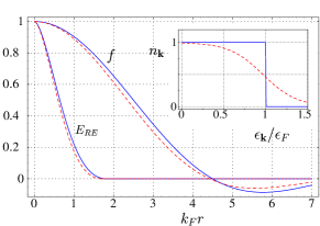
Figure 2: (color online) Relative entropy of entanglement $E_{RE}$ and $f$ as functions of $k_{F}r$ at temperatures $T/T_{F}=0$ (solid line) and $0.2$ (dashed line) for the 3-dimensional electron gas. The inset shows the mean occupation number $n_{\bf k}$ at corresponding temperatures.

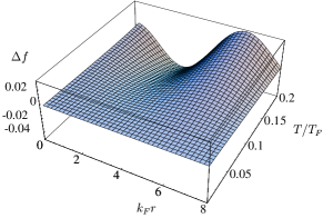
Figure 3: (color online) $\Delta f(r,T)$ as a function of $k_{F}r$ and $T/T_{F}$.

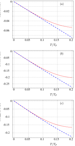
Figure 4: (color online) (a) $\Delta f(r,T)/(T/T_{F})$, (b) $\Delta C(r,T)/(T/T_{F})$, and (c) $\Delta E_{RE}/(T/T_{F})$ versus $T/T_{F}$ at $k_{F}r\sim 1$. The dashed lines are obtained from the Sommerfeld expansion. The solid lines are due to the numerical integration of Eq. (21).

Using the Sommerfeld expansion, we see the temperature dependence of $f(r,T)$ in more detail. At $k_{F}r\sim 1$ we obtain the approximation of $\Delta f(r,T)$ with the order of $T^{2}$ as

$$\Delta f(r,T)\approx\frac{\pi^{2}}{8}\left[\cos(k_{F}r)-\frac{\sin(k_{F}r)}{k_{F}r}\right]\left(\frac{k_{B}T}{\epsilon_{F}}\right)^{2}\,.$$ (22)

Fig. 4 (a) shows the plots of $\Delta f(r,T)$ calculated by the numerical integration of Eq. (21) and the right hand side of Eq. (22) obtained by the the Sommerfeld expansion. We see that at low temperatures the shift of $f$ is the order of $T^{2}$. The change of $f(r,T)$ gives the change of entanglement measures. We calculate $\Delta C(r,T)\equiv C(r,T)-C(r,0)$ written approximately as

$$\Delta C(r,T)\approx\frac{6f(r,0)}{\bigl{[}2-f(r,0)^{2}\bigr{]}^{2}}\Delta f(r,T)\,,$$ (23)

where in derivation we keep only the terms of order $\Delta f(r,T)$. Thus $\Delta C$ is proportional to $T^{2}$ at low temperatures as depicted in Fig. 4 (b). Also we evaluate $\Delta E_{RE}(r,T)\equiv E_{RE}(r,T)-E_{RE}(r,0)$ and find the $T^{2}$ dependence of $\Delta E_{RE}$ at low temperatures as shown in Fig. 4 (c).

Summary.–

In this paper, we obtained the two-particle density matrix of a non-interacting electron gas based on the Green’s function method. It was shown that the two-spin density matrix for a given relative distance between two electrons has the form of a Werner state of which the parameter $p$ is a function of the space density matrix $f$. We presented the relation between the total correlation, the entanglement measures, the classical correlation, and the pair distribution functions. Also we have shown that the entanglement measures change a little bit in proportion to $T^{2}$ at low temperatures and $k_{F}r\sim 1$.

Some remarks should be made. First, in discussion of entanglement of two spins we ignored the space density matrix of electrons. It is interesting to find entanglement measures for identical particles with spatial and internal degrees of freedom. Second, in this work the electron-electron interaction was ignored. It will be our future work to investigate how the electron-electron interaction influences the entanglement measures of electron spins. Finally, how to extract entangled spins out of an electron gas would be another interesting problem.

References

• (1) M. A. Nielsen and I. L. Chuang, Quantum Computation and Quantum Information (Cambridge University Press, Cambridge, 2001)
• (2) V. Vedral, Rev. Mod. Phys. 74, 197 (2002);
• (3) A. Galindo et al., Rev. Mod. Phys. 74, 347 (2002).
• (4) K. M. O’Connor et al., Phys. Rev. A63, 052302 (2001).
• (5) M. C. Arnesen et al., Phys. Rev. Lett. 87, 017901 (2001).
• (6) X. Wang, Phys. Rev. A64, 012313 (2001); 66, 034302 (2002).
• (7) T. J. Osborne et al., Phys. Rev. A66, 032110 (2002).
• (8) A. Osterloh et al., Nature (London) 416, 608 (2002).
• (9) G. Vidal et al., Phys. Rev. Lett. 90, 227902 (2003).
• (10) U. Glaser et al., Phys. Rev. A68, 032318 (2003).
• (11) J. Schliemann et al., Phys. Rev. A64, 022303 (2001).
• (12) R. Pas̆kauskas et al., Phys. Rev. A64, 042310 (2001).
• (13) K. Eckert et al., Ann. Phys. 299, 88 (2002).
• (14) Y. Omar et al., Phys. Rev. A65, 062305 (2002).
• (15) J. R. Gittings et al., Phys. Rev. A66, 032305 (2002).
• (16) H. M. Wiseman et al., Phys. Rev. Lett. 91, 097902 (2003).
• (17) B. Zeng et al., Phys. Rev. A66, 042324 (2002).
• (18) V. Vedral, e-prinit quant-ph/0302040.
• (19) C. N. Yang, Rev. Mod. Phys. 34, 694 (1962).
• (20) A. L. Fetter and J. D. Waleka, Quantum Theory of Many-Particle Systems (McGraw-Hill, New York, 1971).
• (21) A. A. Abrikosov et al., Methods of Quantum Field Theory in Statistical Physics (Dover Publications, New York, 1975).
• (22) G. D. Mahan, Many-Particle Physics, (Plenum Press, New York, 1990).
• (23) P.-O. Löwdin, Phys. Rev. 97, 1490 (1955).
• (24) R. F. Werner, Phys. Rev. A40, 4277 (1989).
• (25) A. Peres, Phys. Rev. Lett. 77, 1413 (1996).
• (26) M. Horodecki et al., Phys. Lett. A 223, 1 (1996).
• (27) R. Horodecki et al., Phys. Lett. A 200, 340 (1995).
• (28) S. Hill et al., Phys. Rev. Lett. 78, 5022 (1997); W. K. Wootters, ibid. 80, 2245 (1998).
• (29) V. Vedral et al., Phys. Rev. Lett. 78, 2275 (1997).
• (30) V. Vedral et al., Phys. Rev. A57, 1619 (1998).
• (31) L. Henderson et al., J. Phys. A 34, 6899 (2001).
• (32) H. Ollivier et al., Phys. Rev. Lett. 88, 017901 (2002); W. H. Zurek, Phys. Rev. A67, 012320 (2003).
• (33) S. Hamieh et al., Phys. Rev. A67, 014301 (2003).