Adiabatic Geometric Phase for a General Quantum State

Abstract

A geometric phase is found for a general quantum state that undergoes adiabatic evolution. For the case of eigenstates, it reduces to the original Berry’s phase. Such a phase is applicable in both linear and nonlinear quantum systems. Furthermore, this new phase is related to Hannay’s angles as we find that these angles, a classical concept, can arise naturally in quantum systems. The results are demonstrated with a two-level model.

Consider a quantum system that depends on some external parameters $\bm{R}$. We are interested in the evolution of its quantum state when the parameters $\bm{R}$ change slowly along a closed path (see Fig.1). For an eigenstate, such an adiabatic evolution accumulates a geometric phase, which reflects the system geometry with the parameter space $\bm{R}$. It is now known as Berry’s phaseberry . Although the same geometry is also embedded in the adiabatic evolution of a general quantum state, including non-eigenstate, it is not clear how a geometric phase can be defined for a general quantum state to extract the system geometry.

In this Letter we introduce a geometric phase for a general quantum state. In the case of eigenstates, this phase can be reduced naturally to the original Berry’s phase. From this reduction, one gains some fresh perspective on the familiar concept of Berry’s phase.

The geometric nature of this new phase is fully explored. Similar to Berry’s phase, it can be regarded as the geometric part of a total phase associated with the adiabatic evolution. In another perspective, it can also be regarded as a part of an Aharonov-Anandan (AA) phaseaa ; chiao . Moreover, the new phase is found to be related to Hannay’s angleshannay in a derivative form. Although Hannay’s angles have long been considered as the counterpart of Berry’s phases in classical mechanics, we find that they can be defined naturally in quantum systems, and be calculated from the new phase. In this sense, this relation unifies two very different concepts, Berry’s phase and Hannay’s angles.

Interestingly, this new geometric phase is also applicable in nonlinear quantum systems. Unlike in linear quantum systems where one may understand the adiabatic evolution of a non-eigenstates in terms of eigenstatesanandan , it is impossible to do the same in nonlinear quantum systems due to the lack of the superposition principle. Therefore, the introduction of this new phase provides a unique and powerful tool to study the adiabatic evolution of a general state in nonlinear quantum systems. Bose-Einstein condensates of dilute atomic gases are an excellent example of nonlinear quantum systemsbec_rmp ; leggett .

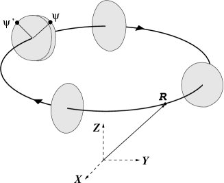
Figure 1: Adiabatic evolution of a quantum state along a closed path in the parameter space of $\bm{R}$. In general, the quantum state does not come back at the end of the evolution, that is, the difference between the start state $\psi$ and the end state $\psi^{\prime}$ is more than a phase. The disks represent the dynamical evolution of a quantum state at a given $\bm{R}$; their different shapes symbolically illustrate the change of the system Hamiltonian with $\bm{R}$. The areas of these disks remain the same, reflecting that the actions $\bm{I}$ are conserved.

In the following discussions, we will proceed with nonlinear quantum systems since linear quantum systems can be regarded as their special cases.

We consider an $N$-level quantum system governed by a general nonlinear Schrödinger equation ($\hbar=1$),

$$i\frac{d}{dt}|\psi\rangle=H(\psi_{j}^{*},\psi_{j};\bm{R})|\psi\rangle\,.$$ (1)

Here $|\psi\rangle=(\psi_{1},\psi_{2},\cdots,\psi_{N})$ is the wave function with $\psi_{j}$ being its $j$th component over an orthonormal basis; the vector $\bm{R}$ represents all the system parameters subject to adiabatic change. We assume that the system is gauge invariant since it is the case of most physical interest. When $H$ is independent of $\psi^{*}_{j}$ and $\psi_{j}$, Eq. (1) is the usual linear Schrödinger equation.

It is well known that the quantum system governed by Eq.(1) mathematically has a canonical classical Hamiltonian structure (e.g., see Refs.weinberg ; heslot ). That is, one can find a Hamiltonian $\mathcal{H}(\psi_{j}^{*},\psi_{j};\bm{R})$ such that Eq. (1) is a set of equations of motion when $\mathcal{H}$ serves the classical Hamiltonian with Poisson brackets $\{\psi_{j}^{*},\psi_{k}\}=i\delta_{jk}$. When the Hamiltonian is bilinear, $\mathcal{H}=\langle\psi|H|\psi\rangle$, the system is linear. With this Hamiltonian structure, the system of Eq.(1) can be classified into integrable or non-integrable in the classical sense. All linear quantum systems are integrable classically.

We focus on the case that Eq.(1) is integrable. In this case, the system at a given $\bm{R}$ has $N$ constants of motion, $\bm{I}=\{I_{1},I_{2},\cdots,I_{N}\}$. They are called actions, whose conjugate variables are angles $\bm{\theta}=\{\theta_{1},\theta_{2},\cdots,\theta_{N}\}$, which change with time linearly as $\bm{\theta}=\bm{\theta}_{0}+\bm{\omega}t$, where $\omega_{j}=\partial\mathcal{H}/\partial I_{j}$. Therefore, at a given $\bm{R}$, the wave function can be expressed as a function of $\{\bm{I},\bm{\theta}\}$, $|\psi\rangle=|\psi(\bm{I},\bm{\theta};\bm{R})\rangle$. Such a parameterization of the wave function in terms of $\{\bm{I},\bm{\theta}\}$ is also very convenient for slowly changing $\bm{R}$. In such an adiabatic evolution, the actions $\bm{I}$ are still conservedarnold while the angles change as $\bm{\theta}(t)=\bm{\theta}_{0}+\int\bm{\omega}(\bm{R})dt+\bm{\alpha}(t)$, where $\bm{\alpha}$ are Hannay’s angleshannay .

With the above observations, we are now mathematically ready to introduce a geometric phase for the adiabatic evolution of a general quantum state $|\psi\rangle$, where the parameters $\bm{R}$ change slowly along a closed path $\mathcal{O}$, as shown in Fig.1. One feature immediately stands out: Except eigenstates, the quantum state generally does not come back to the original state at the end of evolution even though the system Hamiltonian recovers its original form. Moreover, the difference between the initial state and the ending state depends on the choice of the initial state. These features make it difficult to define Berry’s phase and its various generalizations for this evolutionaa ; chiao ; samuel .

To circumvent the obstacle, we use an averaging technique as in the definition of Hannay’s angleshannay . For a quantum states $|\psi\rangle=|\psi(\bm{I},\bm{\theta};\bm{R})\rangle$ adiabatically evolving along the path $\mathcal{O}$, we introduce a geometric phase $\gamma$ as

$$\gamma({\mathcal{O}})=\frac{\oint d\bm{\theta}}{(2\pi)^{N}}\oint_{\mathcal{O}}d\bm{R}\langle\psi(\bm{I},\bm{\theta};\bm{R})|i\frac{\partial}{\partial\bm{R}}|\psi(\bm{I},\bm{\theta};\bm{R})\rangle\,,$$ (2)

where the integration over $\bm{\theta}$ is to average over all possible quantum states with the same actions $\bm{I}$ at a given $\bm{R}$. We emphasize that the integration over $\bm{R}$ in Eq.(2) is done for a fixed $\bm{\theta}$. This new geometric phase $\gamma$ is the same for all the quantum states that has the same actions $\bm{I}$; therefore, it may also be regarded as a geometric phase for an adiabatically evolving manifold. To illustrate and further explore this new phase $\gamma$, we start with some special cases and end with a demonstration with a nonlinear two-level model.

For a quantum system starting at an eigenstate $|E_{n}(\bm{R})\rangle$ defined by

$$H(\bm{R})|E_{n}(\bm{R})\rangle=E_{n}(\bm{R})|E_{n}(\bm{R})\rangle,$$ (3)

it evolves dynamically as $|\psi(t)\rangle=e^{-i\beta(t)}|E_{n}(\bm{R})\rangle$ when $\bm{R}$ changes adiabatically. In this special case, there is only one action, the norm $I=\langle E_{n}(\bm{R})|E_{n}(\bm{R})\rangle$, whose corresponding angle is the phase $\theta=\beta$. Plugging this $|\psi\rangle$ into Eq.(2) and noticing that the partial derivative over $\bm{R}$ does not act on $\theta$ and $I$, we obtain the phase $\gamma$ for eigenstate $|E_{n}\rangle$,

$$\gamma_{n}({\mathcal{O}})=\oint_{\mathcal{O}}d\bm{R}\langle E_{n}(\bm{R})|i\frac{\partial}{\partial\bm{R}}|E_{n}(\bm{R})\rangle\,,$$ (4)

which recovers the original Berry’s phaseberry . Note that Eq.(4) is valid in both linear and nonlinear quantum systems, indicating that the original definition of Berry’s phase can be directly borrowed for nonlinear quantum systems if only eigenstates are considered.

We turn to a general quantum state in linear quantum systems. In this linear case, we can expand the evolving quantum state in terms of the eigenstates,

$$|\psi(t)\rangle=\sum_{n=1}^{N}a_{n}(t)|E_{n}(\bm{R})\rangle\,.$$ (5)

According to the quantum adiabatic theoremmessiah , the occupation probabilities of different eigenstates $|a_{n}|^{2}$ are adiabatic constants. In fact, they are actions $I_{n}=|a_{n}|^{2}$ when the system is regarded mathematically as a classical Hamiltonian system; their corresponding angle variables $\theta_{n}$ are the phases of $a_{n}$’s. With these in mind, computation of Eq.(2) with the state (5) is straightforward. We find that the off-diagonal terms are zeros after the averaging, and the geometric phase $\gamma$ is

$$\gamma({\mathcal{O}})=\sum_{n=1}^{N}|a_{n}|^{2}\gamma_{n}({\mathcal{O}})\,,$$ (6)

where $\gamma_{n}$ is the Berry’s phase of eigenstate $|E_{n}\rangle$. Therefore, in linear quantum systems, the phase $\gamma$ is just a weighted summation of the Berry’s phases of all the eigenstates involved. Interestingly, this kind of weighted summation of Berry’s phases has already been applied in calculating transverse fore on a quantized vortexao and the anomalous Hall conductivity of ferromagnetsyao .

We have so far illustrated the geometric phase $\gamma$ for some simple examples and shown clearly how the phase $\gamma$ as defined in Eq.(2) are related to the well-known Berry’s phase. In the following, we are going to examine the new phase $\gamma$ in a general setting and derive for it a different expression. These efforts reveal that the phase $\gamma$ can be regarded as a geometric part of the total phase of an adiabatic evolution, similar to Berry’s phase.

Imagine an adiabatic evolution of a general quantum state $|\psi\rangle$ along a close path $\mathcal{O}$. Without worrying about whether it is geometric or not, we can always introduce a phase for such an evolution,

$$\beta=i\int_{0}^{T}dt\langle\psi|\frac{d}{dt}|\psi\rangle=i\oint_{\mathcal{O}}\langle\psi|d|\psi\rangle\,,$$ (7)

where $T$ is the total evolution time. We call this phase the total phase of the adiabatic evolution of $|\psi\rangle$. We expand the integrand as

$$\langle\psi(\bm{I},\bm{\theta};\bm{R})|d|\psi(\bm{I},\bm{\theta};\bm{R})\rangle=\langle\psi|\frac{\partial}{\partial\bm{I}}|\psi\rangle\cdot d\bm{I}+$$

$$+\langle\psi|\frac{\partial}{\partial\bm{\theta}}|\psi\rangle\cdot d\bm{\theta}+\langle\psi|\frac{\partial}{\partial\bm{R}}|\psi\rangle\cdot d\bm{R}\,.$$ (8)

For an adiabatic evolution, the actions are conserved so the term involving $\bm{I}$ is zero. Plugging it back into Eq.(7) and averaging it over the initial angles $\bm{\theta}_{0}$, we obtain

$$\bar{\beta} = \oint\frac{d{\bm{\theta}}_{0}}{(2\pi)^{N}}\beta$$ (9)

$$= i\oint_{\mathcal{O}}\frac{\oint d{\bm{\theta}}_{0}}{(2\pi)^{N}}\Big{\{}\langle\psi|\frac{\partial}{\partial\bm{\theta}}|\psi\rangle\cdot d\bm{\theta}+\langle\psi|\frac{\partial}{\partial\bm{R}}|\psi\rangle\cdot d\bm{R}\Big{\}}$$

$$= \bm{I}\cdot\oint_{\mathcal{O}}d\bm{\theta}+\gamma({\mathcal{O}})\,,$$

where we have introduced a new notation $\bar{\beta}$ to stand for the averaged total phase $\beta$. We may also call $\bar{\beta}$ the total phase of an adiabatically evolving manifold. In the derivation, we have noticed for $\gamma$ that the integral over $\bm{\theta}_{0}$ is the same as over a $\bm{\theta}$ at any given $\bm{R}$. We have also used that

$$I_{j}=\frac{1}{2\pi}\oint d{\theta_{0}}_{j}\langle\psi|\frac{\partial}{\partial\theta_{j}}|\psi\rangle\Big{|}_{\theta_{j}={\theta_{0}}_{j}}$$ (10)

is the action of the motion associated with angle $\theta_{j}$. Note that this expression is also the Aharonov-Anandan (AA) phase of the cyclic state, describing the motion associated with the angle variable $\theta_{j}$liu .

The equation (9) shows that the averaged total phase $\bar{\beta}$ has two parts: a dynamical part involving action-angle variables and a geometric part that is exactly our new phase $\gamma$. For the special case of eigenstate $|\psi\rangle=|E_{n}\rangle$, since there is only one non-zero action $I=\langle E_{n}|E_{n}\rangle$, we have

$$\bar{\beta}=\beta=\langle E_{n}|E_{n}\rangle\int_{0}^{T}\omega_{n}dt+\gamma_{n}(\mathcal{O})\,.$$ (11)

It recovers the well-known fact that Berry’s phase is the geometric part of the total phase of an adiabatic evolution of an eigenstateberry .

We re-write Eq.(9) and obtain another expression for the geometric phase $\gamma$,

$$\gamma({\mathcal{O}})=\bar{\beta}-\bm{I}\cdot\oint_{\mathcal{O}}d\bm{\theta}\,.$$ (12)

This complicated expression turns out to be easier to be implemented numerically; we will use it to compute the results shown in Fig.2.

One can repeat the derivation from Eq.(7) to Eq.(12) in the projective Hilbert space. In this situation, the total phase Eq.(7) becomes an AA phase, and the phase $\gamma$ can then be regarded as the geometric part of the AA phase associated with the parameter space.

There is another interesting angle looking into the new phase $\gamma$. As already mentioned, the system described in Eq.(1) has a canonical classical Hamiltonian structure. With this classical structure, we can introduce naturally Hannay’s angles, a classical concept, into quantum systems. Following the expression for Hannay’s angles in Ref.hannay ; semi1 ; semi2 , we find that these angles in our quantum system (1) are related to the phase $\gamma$ by

$$\bm{\alpha}({\mathcal{O}})=-\frac{\partial}{\partial\bm{I}}\gamma({\mathcal{O}})\,.$$ (13)

In linear quantum systems, these Hannay’s angles differ from Berry’s phases of eigenstates only by a sign, $\alpha_{n}=-\gamma_{n}$, according to Eq.(6). Note the relation (13) is very similar in form to the semiclassical relation between Hannay’s angles and Berry’s phases derived in Ref.semi1 ; semi2 although they are two very different relations. So far, it is not clear why the similarityjie .

Finally, we demonstrate the geometric phase $\gamma$ with a nonlinear two-level model as given by

$$i\frac{d\varphi_{1}}{dt} = \Big{[}c|\varphi_{2}|^{2}+\frac{Z}{2}\Big{]}\varphi_{1}+\frac{X-iY}{2}\varphi_{2}\,,$$ (14)

$$i\frac{d\varphi_{2}}{dt} = \Big{[}c|\varphi_{1}|^{2}-\frac{Z}{2}\Big{]}\varphi_{2}+\frac{X+iY}{2}\varphi_{1}\,.$$ (15)

This simple model can be used to describe the Josephson effect of Bose-Einstein condensates residing in a double-well potentialleggett ; walls . The complex coupling constant, as denoted by $X$ and $Y$, can be realized in experiment through phase imprinting on one of the two wellsimprint .

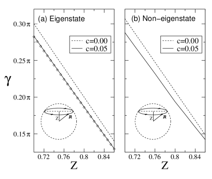
Figure 2: Geometrical phases $\gamma$ of the nonlinear two-level model (14,15): (a) the lower eigenstate and (b) the non-eigenstate near the lower eigenstate. The non-eigenstate has an action (or AA phase) of $I=0.005$. The insert shows the closed path $\mathcal{O}$ used which is a circle on a unit sphere with $Z$ fixed. The circle is traversed with a rate of 0.001. The results for eigenstates are compared to the analytical expression of Eq.(16) (denoted by diamonds): a very good match is found.

We first look at the geometric phase $\gamma$ for eigenstates of this nonlinear quantum system. This is to find all the eigenstates $|E_{n}(\bm{R})\rangle$ for a closed path $\mathcal{O}$, and use them to calculate the phase with Eq.(4). Both steps could be done numerically; fortunately for this simple case, analytical results can be obtained. When the path is restricted on the unit sphere $X^{2}+Y^{2}+Z^{2}=1$, we find that the phases for these nonlinear eigenstates are

$$\gamma({\mathcal{O}})=\int_{\partial S={\mathcal{O}}}\frac{\eta^{3}(\bm{R}+c\eta\hat{z})\cdot d\bm{S}}{(c\eta+Z)^{2}(c\eta^{3}+Z)}\,,$$ (16)

where $\hat{z}$ is the unit vector along the $z$-axis and $\eta$ is one of the real roots of

$$c^{2}\eta^{4}+2cZ\eta^{3}+(1-c^{2})\eta^{2}-2cZ\eta-Z^{2}=0\,.$$ (17)

Different real roots $\eta$ correspond to different eigenstates. It is clear that Eq.(17) can have more than two real roots, indicating that there can be more than two eigenstatesnlz . Here we limit ourselves to the situations where Eq.(17) has only two real roots. For the path $\mathcal{O}$ that is a circle with a fixed $Z$, the geometric phase in Eq.(16) becomes $\gamma=(1-\eta)\pi$. The diamonds in Fig.2 are calculated with Eq.(16), showing how $\gamma$ for the lower eigenstate changes with $Z$.

For a general quantum state, we have to resort to numerical means. The path $\mathcal{O}$ is picked to be a circle with fixed $Z$. We then solve Eqs.(14,15) numerically after choosing a changing rate $v=0.001$ for the parameters $\bm{R}=\{X,Y,Z\}$. The evolving states are recorded and used to compute the phase $\gamma$ with Eq.(12), where the averaging is done for different initial states with the same action (or AA phase) $I$. Results for $c=0.05$ are plotted in Fig.2, showing how the phase changes with $Z$. Computation is done for both eigenstate and non-eigenstate and the results (solid lines) are compared to the phases for the linear case $c=0.0$ (dashed lines). The changing rate of $\bm{R}$ ($v=0.001$) is slow enough to be considered as adiabatic. This is witnessed by the good fit between the solid line and the diamonds in Fig.2(a) as the diamonds are the analytical results of Eq.(16).

In summary, we have introduced a geometric phase for a general adiabatically evolving quantum state. The new phase to certain extent unifies two different concepts, Berry’s phase and Hannay’s angles. It is very interesting to find potential applications for this new geometric phase while its properties are being further explored.

We acknowledge the support of NSF (DMR-0306239), R. A. Welch Foundation, and LDRD of ORNL, managed by UT-Battelle, LLC for the USDOE (DE-AC0500OR22725).

References

- (1) M.V. Berry, Proc. R. Soc. London A 392, 45 (1984).
- (2) Y. Aharonov and J. Anandan, Phys. Rev. Lett. 58, 1593 (1987).
- (3) J.C. Garrison and R.Y. Chiao, Phys. Rev. Lett. 60, 165 (1988); J. Anandan, Phys. Rev. Lett. 60, 2555 (1988).
- (4) J.H. Hannay, J. Phys. A 18, 221 (1985).
- (5) J. Anandan and L. Stodolsky, Phys. Rev. D 35, 2597 (1987).
- (6) F. Dalfovo, S. Giorgini, L.P. Pitaevskii, and S. Stringari, Rev. Mod. Phys. 71, 463 (1999).
- (7) A.J. Leggett, Rev. Mod. Phys. 73, 307 (2001).
- (8) A. Heslot, Phys. Rev. D 31, 1341 (1985).
- (9) S. Weinberg, Phys. Rev. Lett. 62, 485 (1989); S. Weinberg, Ann. Phys. 194, 336 (1989).
- (10) V.I. Arnol’d, Mathematical Methods of Classical Mechanics (Springer-Verlag, Berlin, 1978).
- (11) J. Samuel and R. Bhandari, Phys. Rev. Lett. 60, 2339 (1988).
- (12) A. Messiah, Quantum mechanics, (Dover, 2000).
- (13) D.J. Thouless, Ping Ao, and Qian Niu, Phys. Rev. Lett. 76, 3758 (1996).
- (14) Yugui Yao, L. Kleinman, A.H. MacDonald, Jairo Sinova, T. Jungwirth, Ding-sheng Wang, Enge Wang, Qian Niu, Phys. Rev. Lett. 92, 037204 (2004).
- (15) Jie Liu, Biao Wu, and Qian Niu, Phys. Rev. Lett. 90, 170404 (2003).
- (16) M.V. Berry, J. Phys. A 18, 15 (1985).
- (17) J. Anandan, Phys. Lett. A 129, 201 (1988).
- (18) Jie Liu, Bambi Hu, and Baowen Li, Phys. Rev. Lett. 81, 1749 (1998); Jie Liu, Bambi Hu, and Baowen Li, Phys. Rev. A 58, 3448 (1998).
- (19) G.J. Milburn, J. Comey, E.M. Wright, and D.F. Walls, Phys. Rev. A 55, 4318.
- (20) J. Denschlag, J.E. Simsarian, D.L. Feder, C.W. Clark, L.A. Collins, J. Cubizolles, L. Deng, E.W. Hagley, K. Helmerson, W.P. Reinhardt, S.L. Rolston, B.I. Schneider, and W.D. Phillips, Science 287, 97 (2000).
- (21) Biao Wu and Qian Niu, Phys. Rev. A 61, 023402 (2000).