Qubit Channels Which Require Four Inputs to Achieve Capacity:
Implications for Additivity Conjectures

Abstract

An example is given of a qubit quantum channel which requires four inputs to maximize the Holevo capacity. The example is one of a family of channels which are related to 3-state channels. The capacity of the product channel is studied and numerical evidence presented which strongly suggests additivity. The numerical evidence also supports a conjecture about the concavity of output entropy as a function of entanglement parameters. However, an example is presented which shows that for some channels this conjecture does not hold for all input states. A numerical algorithm for finding the capacity and optimal inputs is presented and its relation to a relative entropy optimization discussed.

1 Introduction

The Holevo capacity $C(\Gamma)$ of a 1-qubit quantum channel $\Gamma$ is defined as the supremum over all possible ensembles of 1-qubit density matrices $\rho_{i}$ and probability distribution $p_{i}$ of

$$S(\Gamma(\rho))-\sum_{i}p_{i}S(\Gamma(\rho_{i}))$$

where $\rho=\sum_{i}p_{i}\rho_{i}$ is the average input and $S(\sigma)=-{\rm Tr}(\sigma\log\sigma)$ denotes the von Neumann entropy. The Holevo capacity gives the maximum rate at which classical information can be transmitted through the quantum channel [6, 23] using product inputs, but permitting entangled collective measurements. It is a consequence of Carathéodory’s Theorem and the convex structure of this problem (as discussed in the next section) that the above supremum can be replaced with the maximum over four input pairs of $(\rho_{i},p_{i})$. (Davies [2] seems to have been the first to recognize the relevance of Carathéodory’s Theorem to problems of this type in quantum information theory; explicit application to quantum capacity optimization appeared in [5]). It was demonstrated in [11] that there exist qubit channels requiring three input states to attain the maximum. However, it was left open whether or not there are 1-qubit channels requiring four input states to achieve the maximum. This paper shows that such 4-input channels do exist by presenting an example. The computation of this capacity is a nonlinear programming problem. Unlike the classical channel capacity computation, this problem is much harder, especially in a point that the classical case is the maximization of a concave function while the quantum case is the maximization of a function which is concave with respect to probability variables, as in the classical case, and is convex with respect to state variables. As for algorithms to compute the capacity by utilizing the special structure of the problem, [15] developed an alternating-type algorithm, by extending the well-known Arimoto-Blahut algorithm for the classical channel capacity, and is implemented in [17] to check the additivity. Use of interior-point methods is suggested in [7]. A method is presented in [26] for computing the capacity by combining linear programming techniques, including column generation, with non-linear optimization. In this paper, we present an approximation algorithm to compute the capacity of a 1-qubit channel; our algorithm plays a key role in finding a 4-state channel numerically.

Although $C(\Gamma)$ plays an important role in quantum information theory, it is not known whether or not using entangled inputs might increase the capacity. This is closely related to the question of the additivity of $C(\Gamma\otimes\Gamma)$, which is now known [18, 13, 27] to be equivalent to other conjectures including additivity of entanglement of formation. In addition to being of interest in their own right, 4-state channels are good candidates for testing the additivity conjecture of the Holevo capacity for qubit channels. We present numerical evidence for additivity which, in view of special properties of the channels, gives extremely strong evidence for additivity of both capacity and minimal output entropy for qubit channels. Both results would follow from a new conjecture (which appeared independently in [3]) about concavity of entropy as a function of entanglement parameters. Using a different channel, we show that this conjecture is false, at least in full generality.

The paper is organized as follows. Basic background, definitions and notation for convex analysis and qubit channels is presented in Sections 2 and 3, respectively. Numerical results for the 4-state channel and the algorithm used to obtain them are described in Sections 4 and 5. Some intuition about the properties of 3-state and 4-state channels is presented in Section 6 and shown to lead to additional examples of 4-state channels. In Section 7, different views of the capacity optimization are discussed and shown to be related to a relative entropy optimization. The additivity analysis and counterexample to the concavity conjecture are given in Section 8. Throughout this paper, the base of the logarithm is 2.

2 Convex Analysis

The function to be maximized in the Holevo capacity has a special form, to which general convex analysis may be applied. Based on [20], this section discusses the problem in this form.

Suppose $D$ is a $d$-dimensional bounded, closed convex set in ${\bf R}^{d}$, and $f$ is a closed, concave function from $D$ to ${\bf R}$. We are interested in the following infinite programming problem.

$$F=\sup_{\mbox{\footnotesize\boldmath$x$}_{i}\in D,\,p_{i}}(f(\overline{\mbox{\boldmath$x$}})-\sum_{i}p_{i}f(\mbox{\boldmath$x$}_{i}))$$ (1)

where $\overline{\mbox{\boldmath$x$}}=\sum_{i}p_{i}\mbox{\boldmath$x$}_{i}$, $\sum_{i}p_{i}=1$, and $p_{i}\geq 0$. This infinite mathematical programming problem can be reduced to a finite mathematical programming with $d+1$ pairs of $(x_{i},p_{i})$ as follows.

For such a closed, concave function $g$ over $D$, its closure of convex hull function $\mbox{cl}~{}\mbox{conv}~{}g$ is the greatest convex function majorized by $g$ (p.36, p.52 in [20]). In our case, further using Carathéodory’s Theorem (Theorem 17.1 in [20]), it is expressed as

$$\mbox{cl}~{}\mbox{conv}~{}g(\mbox{\boldmath$x$})=\min\bigg{\{}\,\sum_{i=1}^{d+1}p_{i}g(\mbox{\boldmath$x$}_{i}):\mbox{\boldmath$x$}=\sum_{i=1}^{d+1}p_{i}\mbox{\boldmath$x$}_{i},\ \sum_{i=1}^{d+1}p_{i}=1,\ \mbox{\boldmath$x$}_{i}\in D,\ p_{i}\geq 0\ (i=1,\ldots,d+1)\,\bigg{\}}$$

It is then seen that the problem (1) is reduced to the following Fenchel-type problem (cf. Fenchel’s duality theorem, section 31, [20]).

$$\max_{\mbox{\footnotesize\boldmath$x$}\in D}(f(\mbox{\boldmath$x$})-\mbox{cl}~{}\mbox{conv}~{}f(\mbox{\boldmath$x$})),$$ (2)

By virtue of nice properties of minimizing convex functions (e.g., Theorem 27.4 in [20]), the optimality of a solution to this problem is well-known:

Lemma 1

$\widetilde{\mbox{\boldmath$x$}}$ is optimum in (2) if and only if there is $\xi\in{\bf R}^{d}$ such that, for any $\mbox{\boldmath$x$}\in D$,

$$\xi^{\rm T}(\mbox{\boldmath$x$}-\widetilde{\mbox{\boldmath$x$}})+\mbox{cl}~{}\mbox{conv}~{}f(\widetilde{\mbox{\boldmath$x$}})\leq\mbox{cl}~{}\mbox{conv}~{}f(\mbox{\boldmath$x$})\leq f(\mbox{\boldmath$x$})\leq\xi^{\rm T}(\mbox{\boldmath$x$}-\widetilde{\mbox{\boldmath$x$}})+f(\widetilde{\mbox{\boldmath$x$}}).$$

Furthermore, when $f$ is strictly concave, there is a unique optimum solution.

The above discussions can be summarized in the form of problem (1) as follows:

Corollary 1

In the infinite mathematical programming problem (1), the supremum can be replaced with the maximum over $d+1$ pairs of $(\mbox{\boldmath$x$}_{i},p_{i})$. If there exist $d+1$ affinely independent points $\mbox{\boldmath$x$}_{i}$ $(i=1,\ldots,d+1)$ such that a unique hyperplane passing through $(\mbox{\boldmath$x$}_{i},f(\mbox{\boldmath$x$}_{i}))$ $(\mbox{\boldmath$x$}_{i}\in D$, $i=1,\ldots,d+1)$ in ${\bf R}^{d+1}$ is a supporting hyperplane to the convex set $\{\,(\mbox{\boldmath$x$},y)\mid\mbox{\boldmath$x$}\in D,\ \mbox{cl}~{}\mbox{conv}~{}f(\mbox{\boldmath$x$})\leq y\leq f(\mbox{\boldmath$x$})\,\}$ from below, and, for these $\mbox{\boldmath$x$}_{i}$ $(i=1,\ldots,d+1)$,

$$\max\{\,f(\sum_{i=1}^{d+1}p_{i}\mbox{\boldmath$x$}_{i})-\sum_{i=1}^{d+1}p_{i}f(\mbox{\boldmath$x$}_{i})\mid\sum_{i=1}^{d+1}p_{i}=1,\ p_{i}\geq 0\,\}$$

is attained with $p_{i}>0$ for all $i=1,\ldots,d+1$, then a set of $d+1$ pairs of $(\mbox{\boldmath$x$}_{i},p_{i})$ is an optimum solution to (1).

3 Set-up

In the calculation of channel capacity for state on ${\bf C^{d}}$, the convex set $D$ is the set of density matrices, i.e., the set of $d\times d$ positive semi-definite matrices with trace $1$. This is isomorphic to a convex subset of ${\bf R}^{d^{2}-1}$. A channel $\Gamma(\rho)$ is described by a special type of linear map on the set of density matrices, namely, one which is also completely positive and trace-preserving.

In the case of qubits, it is well-known that the set $D$ of density matrices is isomorphic to the unit ball in ${\bf R}^{3}$ via the Bloch sphere representation. We will use the notation $\rho(x,y,z)$ to denote the density matrix $\frac{1}{2}[I+x\sigma_{x}+y\sigma_{y}+z\sigma_{z}]$. It was shown in [9] that, up to specification of bases, a qubit channel can be written in the form

$$\Gamma[\rho(x,y,z))]=\rho(\lambda_{1}x+t_{1},\lambda_{2}y+t_{2},\lambda_{3}z+t_{3}).$$ (3)

which gives an affine transformation on the Bloch sphere. In fact, it maps the Bloch sphere $\{\,(x,y,z)\mid x^{2}+y^{2}+z^{2}\leq 1\,\}$ to an ellipsoid with axes of lengths $\lambda_{1},\lambda_{2},\lambda_{3}$ and center $t_{1},t_{2},t_{3}$. Complete positivity poses additional constraints on the parameters $\{\lambda_{k},t_{k}\}$ which are given in [22].

The strict concavity of $S(\rho)$ implies that $S[\Gamma(\rho)]$ is also strictly concave for channels which are one-to-one. In the case of qubits, this will hold unless the channel maps the Bloch sphere into a one- or two-dimensional subset, which can only happen when one of the parameters $\lambda_{k}=0$.

4 Numerical results

The theory in Section 2 can be used to calculate the capacity with $f(\rho)=S[\Gamma(\rho)]$. We are interested in qubit channels with all $\lambda_{k}\neq 0$ so that strict concavity holds. Then the optimization problem as formulated in (2) has a unique solution. However, in the form (1) as restricted in Corollary 1, it may have multiple optimum solutions when the hyperplane passes through more than $d+1$ such points.

Numerical optimization to compute the capacity of this channel was initially performed by utilizing a mathematical programming package NUOPT [14] of Mathematical Systems Inc. These results, accurate to at most 7-8 significant figures, were further refined by using them as starting points in a program to find a critical point of the capacity by applying Newton’s method to the gradient. The results are shown in Table LABEL:tab:4st.

$$\Gamma[\rho(x,y,z)]=\rho(0.6x+0.21,0.601y,0.5z+0.495)~{}~{}\qquad~{}~{}\text{capacity}=0.3214851589$$

$$S(\Gamma(\rho_{i}(x,y,z)))-\xi^{\rm T}\Gamma(\rho_{i})=.9785055621~{}~{}~{}\forall~{}i\qquad H[\Gamma(\rho_{i}),\Gamma(\rho_{{}^{\rm Av}})]=0.3214851589~{}~{}~{}\forall~{}i$$

$$\begin{array}[]{ccrc}\text{probability}&\text{optimal input }(x,y,z)&\phi{}{}{}&\theta\\ 0.2322825705&(~{}~{}0.2530759862,-0.0000000000,~{}~{}0.9674464043)&~{}~{}~{}0.127929&0\\ 0.2133220819&(~{}~{}0.9783950999,~{}0.0000000000,~{}~{}0.2067438718)&0.681275&0.0\\ 0.2771976738&(-0.4734087533,~{}~{}0.8646461389,-0.1681404376)&0.869870&~{}2.071131\\ 0.2771976738&(-0.4734087533,-0.8646461389,-0.1681404376)&0.869870&-2.071131\\ \text{average}&(~{}~{}0.0050428099,~{}~{}0.0000000000,~{}~{}0.1756076944)&\end{array}$$

To verify that these results give a true 4-state optimum, the function $S(\Gamma(\rho(x,y,z)))-\xi^{{}^{\rm T}}\Gamma(\rho)$ was computed and plotted with $\xi=(-0.0396622022,0,-0.9621071440)$. These results are shown in Figure 1 and confirm the condition that the hyperplane $(\xi,-1)\cdot(x,y,z,w)=-0.9785055621$ passes through the four points $((x_{i},y_{i},z_{i},S(\Gamma[\rho(x_{i},y_{i},z_{i})]))$ and the condition that the hyperplane lies below the surface $(x,y,z,S(\Gamma[\rho(x,y,z)])$ in ${\bf R}^{4}$. (The components $\xi_{x},\xi_{y},\xi_{z}$ of $\xi$ are obtained by solving the four simultaneous equations $\xi^{T}\cdot\Gamma(\rho_{k})+\xi_{0}=S(\Gamma[\rho(x_{i},y_{i},z_{i})])\;(k=1,2,3,4)$ for the variables $(\xi_{x},\xi_{y},\xi_{z},\xi_{0})$. ) As discussed in Section 7 this is equivalent to a relative entropy optimization.

In addition, the optimal three-state capacity was also computed and shown to be $<0.321461$ which is strictly less than the 4-state capacity of 0.321485. Details for the 3-state capacity can be found in Table 2 (Section 6). As an optimization problem, the capacity has other local maxima in addition to the 3-state and 4-state results discussed above. For example, there are several 2-state optima, but these have lower capacity and are not relevant to the work presented here.

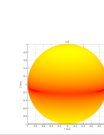
inputs $(\rho(x,y,z)$ on the two hemispheres of the Bloch sphere.   left: $x>0$    right: $x<0$

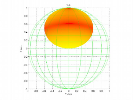
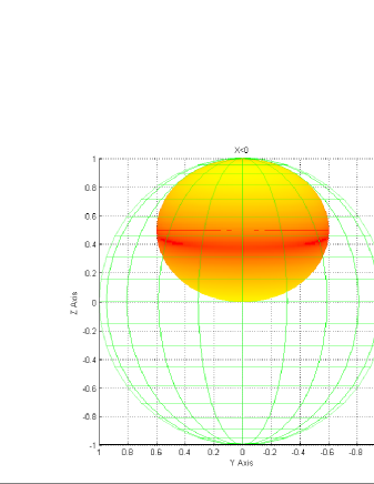
output states $\Gamma(\rho(x,y,z))$ on the image ellipsoid.   left: $x>0$    right: $x<0$

Scale for interpretation $F(x,y,z)=S(\Gamma[\rho(x,y,z)])-\xi^{\rm T}\Gamma[(\rho(x,y,z)])$
    
Scale for interpretation as $H[\Gamma(\omega),\Gamma(\rho^{4}_{{}^{\rm Av}})]$

Figure 1: Depiction of $F(x,y,z)=S(\Gamma[\rho(x,y,z)])-\xi^{\rm T}\Gamma[(\rho(x,y,z)])$ and relative entropy $H[\Gamma(\omega),\Gamma(\rho^{4}_{{}^{\rm Av}})]=1.299989-F(x,y,z)$ with respect to optimal average output in terms of color (or grey scale) on the boundary of the Bloch sphere and its image.

5 Approximation Algorithm to Compute the Holevo Capacity

To find the 4-state channel given above, the following approximation algorithm was repeatedly applied with various parameters. This approximation algorithm is almost sufficient to compute the Holevo capacity of a 1-qubit channel in practice.

Recall that the problem (1) is an infinite mathematical programming problem. As far as all $\mbox{\boldmath$x$}_{i}\in D$ are considered, this infinite set may be regarded as fixed, leaving only $p_{i}$ as variables. The objective function is concave with respect to $p_{i}$, which is quite nice to solve, although the problem is still an infinite one.

For a 1-qubit channel, owing to the concavity of the von Neumann entropy, in the formulation (1), $x$ can be restricted to a pure state, i.e., $x^{2}+y^{2}+z^{2}=1$ in terms of the Bloch sphere. The sphere is two-dimensional, and the convex hull of a square mesh of $k(k+1)$ points $(\sin(\theta_{j})\cos(\mu_{l}),\sin(\theta_{j})\sin(\mu_{l}),\cos(\theta_{j}))$ with $\theta_{j}=j\pi/k$, $\mu_{l}=2l\pi/k$ $(j=0,...,k$; $l=0,\ldots,k-1)$ is quite a good polyhedral approximation. For $j=0,k$ and any $l$, points become $(0,0,1)$ and $(0,0,-1)$, and the total number of points is $k^{2}-k+2$ (See Fig.2, left). Then, considering the problem of type (1) for these $k^{2}-k+2$ points with constraints $\sum_{i=1}^{k^{2}-k+2}p_{i}=0$, $p_{i}\geq 0$, the maximum to this $(k^{2}-k+2)$-dimensional concave maximization problem gives a close lower bound to the real maximum of the original problem.

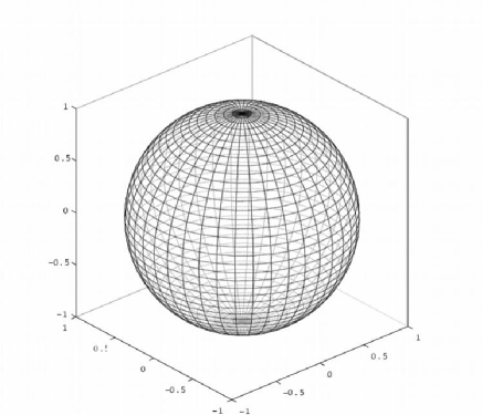
Figure 2: (left) A polyhedral approximation of the sphere for $k=40$. It has $k^{2}-k+2=1562$ points. (right) Approximation values by $(k^{2}-k+2)$-point mesh. The horizontal axis is a log plot of $k$, and the vertical axis is a log plot of the difference to the optimum value in bit. A line $y=0.05/x^{2}$ is drawn for reference.

Interior-point methods can be applied to this high-dimensional concave maximization programming problem (e.g., [19]). Computational results from NUOPT are shown in Fig.2, right, from which this approximation approach provides values sufficiently close to the Holevo capacity in practice.

6 Heuristic construction of a 4-state channel

The existence of four state channels of the type found above can be understood as emerging from small deformations of 3-state channels with a high level of symmetry. As noted above, a channel of the form (3) maps the Bloch sphere to an ellipsoid with axes of lengths $\lambda_{1},\lambda_{2},\lambda_{3}$ and center $t_{1},t_{2},t_{3}$. When $t_{1}=t_{2}=t_{3}$, the ellipsoid is centered at the original and the capacity is achieved with a pair of orthogonal inputs which map to the endpoints of the longest axis of the ellipsoid. However, when some $t_{k}$ are non-zero, this no longer holds and it can even happen that the capacity is achieved with a pair of orthogonal inputs which map to the endpoints of the shortest axis (as for the example $\Gamma[\rho(x,y,z))]=\rho(0.55x,0.55y,0.5z+0.5)$.) By finding parameters which balance these situations, 3-state channels were constructed in [11] .

One of the 3-state channels in [11] is

$$\Gamma(\rho(x,y,z))=\rho(0.6x,0.6y,0.5z+0.5)$$ (4)

which has rotational symmetry about the z-axis of the Bloch sphere. This allows one to analyze the problem in two-dimensional plane, but with the limitation that at most a 3-state channel can be found. Although the analysis of this channel was performed in the $x$-$z$ plane, one could, instead, choose the optimal inputs to lie any plane containing the $z$-axis, e.g., the $y$-$z$ plane. Moreover, if one replaces the two inputs $(\pm 0.93681,\,0,\,-0.34984)$, each with probability 0.29885, by any three or more states with $z=-0.34984$ which also average to $(0,0,-0.34984)$ the capacity is unchanged. However, only three inputs are actually necessary to achieve this capacity.

To find a true 4-state channel, the symmetry must be lowered so that the full 3-dimensional geometry of the Bloch sphere is required. The channel (4) was obtained as a convex combination of an amplitude damping channel with $\lambda_{1}=\lambda_{2}=\frac{1}{\sqrt{2}}\approx 0.707$ and a shifted depolarizing channel with $\lambda_{1}=\lambda_{2}=0.5$. Thus, once could expect to make minor changes to $\lambda_{1}$ and/or $\lambda_{2}$ without violating the CP condition [5, 9, 22] of $(\lambda_{1}\pm\lambda_{2})^{2}\leq(1\pm\lambda_{3})^{2}+t_{3}^{2}=\frac{9\pm 1}{4}$ for channels with $t_{1}=t_{2}=0$. Letting $\lambda_{1}=0.6,\lambda_{2}=0.601$ gives a channel with reflection symmetry across the $x$-$z$ and $y$-$z$ planes. Its capacity will require three input states which lie in the $y$-$z$ plane as shown in Table  2. We now wish to further reduce the symmetry by shifting the ellipsoid. To do so, one must first decrease $\lambda_{3}$ or $t_{3}$. We consider the channel

$$\Gamma[\rho(x,y,z))]=\rho(0.6x,0.601y,0.5z+0.495)$$ (5)

which is still CP and requires three input states which lie in the $y$-$z$ plane as shown in Table  2.

$\Gamma(\rho(x,y,z))=\rho(0.6x,0.6y,0.5z+0.5)$                  $C(\Gamma)=0.324990$

$$\begin{array}[]{ccc}\text{probability}&\text{inputs}&\text{outputs}\\ 0.402338&(0.000000,0.000000,1.000000)&(0.000000,0.000000,1.000000)\\ 0.298830&(0.936786\cos\vartheta,0.936786\sin\vartheta,-0.349902)&(0.562072\cos\vartheta,0.562072\sin\vartheta,0.3250492)\\ 0.298830&(-0.936786\cos\vartheta,-0.936786\sin\vartheta,-0.349902)&(-0.562072\cos\vartheta,-0.562072\sin\vartheta,0.325049)\\ \text{average}&(0.000000,0.000000,0.193215)&(0.000000,0.000000,0.596608)\end{array}$$

The ellipsoid is symmetric about the $z$-axis so that the optimal inputs can be chosen to lie in any plane containing the $z$-axis. For $\vartheta=\pi/2$, $x=0$ and the optimal inputs lie in the $y$-$z$ plane; for $\vartheta=0$, $y=0$ and the optimal inputs lie in the $x$-$z$ plane.
  
  
$\Gamma(\rho(x,y,z))=\rho(0.6x,0.601y,0.5z+0.5)$                  $C(\Gamma)=0.325555$

$$\begin{array}[]{ccc}\text{probability}&\text{inputs}&\text{outputs}\\ 0.380692&(0.000000,0.000000,1.000000)&(0.000000,0.000000,1.000000)\\ 0.309653&(0.000000,0.952435,-0.304740)&(0.000000,0.572413,0.347630)\\ 0.309653&(0.000000,-0.952435,-0.304740)&(0.000000,-0.572414,0.347630)\\ \text{average}&(0.000000,0.000000,0.191964)&(0.000000,0.000000,0.595982)\end{array}$$

The longest axis of the ellipsoid is parallel to the $y$-axis, and optimal inputs lie in the $y$-$z$ plane.
  
  
$\Gamma(\rho(x,y,z))=\rho(0.6x,0.601y,0.5z+0.495)$                  $C(\Gamma)=0.320535$

$$\begin{array}[]{ccc}\text{probability}&\text{inputs}&\text{outputs}\\ 0.146660&(0.000000,0.000000,1.000000)&(0.000000,0.000000,0.995000)\\ 0.426670&(0.000000,0.999687,0.025034)&(0.000000,0.600811,0.507517)\\ 0.426670&(0.000000,-0.999687,0.025034)&(0.000000,-0.600811,0.507517)\\ \text{average}&(0.000000,0.000000,0.168022)&(0.000000,0.000000,0.579011)\end{array}$$

The longest axis of the ellipsoid is parallel to the $y$-axis, and optimal inputs lie in the $y$-$z$ plane.
  
  
$\Gamma(\rho(x,y,z))=\rho(0.6x+0.021,0.601y,0.5z+0.495)$                  $C_{3}(\Gamma)=0.3214609877$

$$\begin{array}[]{cccc}\text{probability}&\text{inputs}&\text{outputs}&S[\Gamma(\rho)]\\ 0.213290&(0.252867,0.000000,0.9675017)&(0.172720,0.000000,0.978751)&0.029992\\ 0.366051&(0.978544,0.000000,0.206036)&(0.608127,0.000000,0.598018)&0.379029\\ 0.420657&~{}(-0.967649,0.000000,-0.252299){}&~{}(-0.559590,0.000000,0.368851)&0.645884{}\\ \text{average}&(0.005083,0.000000,0.1756493)&(0.024050,0.000000,0.582825)&0.738297\end{array}$$

A shift in the $x$-direction offsets the slightly greater length parallel to the $y$-axis so that the restricted 3-state optimization inputs lie in the $x$-$z$ plane. However, the 3-state capacity is less than that for the unrestricted problem which requires four input states.

Table 2: Optimal 3-state ensembles for various channels

We now shift the channel in the x-direction and study

$$\Gamma[\rho(x,y,z))]=\rho(0.6x+0.21,0.601y,0.5z+0.495)$$ (6)

The CP condition [12,13] for a channel of the form

$$\Gamma[\rho(x,y,z))]=\rho(0.6x+t_{1},0.601y,0.5z+0.495)$$ (7)

reduces to $\det(I-R^{T}R)\geq 0$ where $R=\begin{pmatrix}\frac{t_{1}}{\sqrt{(1.995)(0.005)}}&\frac{1.201}{\sqrt{(1.995)(1.005)}}\\ &\\ \frac{-0.001}{\sqrt{(0.995)(0.005)}}&\frac{t_{1}}{\sqrt{(0.995)(1.005)}}\end{pmatrix}.$ This gives the quartic inequality $0.2805326349-101.0098436\,t_{1}^{2}+100.2531329\,t_{1}^{4}\geq 0$ which holds for $|t_{1}|\leq 0.05277$. .

Although small enough to satisfy the CP condition, a shift of $t_{1}=0.021$ is sufficient to return the (restricted) 3-state optimum to the $x$-$z$ plane across which the image has reflection symmetry. In fact, the inputs $\rho(x,y,z)$ and $\rho(x,-y,z)$ have the same output entropy. Moreover, replacing all inputs $\rho_{i}(x,y,z)$ by $\rho_{i}(x,-y,z)$ leaves the capacity unchanged. Therefore, either all optimal inputs lie in the $x$-$z$ plane or the set of optimal inputs contains pairs of the form $\rho(x,\pm y,z)$ with the same probability. (This follows easily from a small modification of the convexity argument in [11]. ) Let

$$\chi[\pi_{1},\rho_{1},\pi_{2},\rho_{2},\pi_{3},\rho_{3}]=S\big{(}\textstyle{\sum}_{i}\pi_{i}\rho_{i}\big{)}-\sum_{i}\pi_{i}S(\rho_{i}).$$ (8)

For simplicity, assume that $y_{1}=y_{2}=0$, but $y_{3}\neq 0$. Let $\pi_{4}=\pi_{3}$ and $\rho_{4}=\rho(x_{3},-y_{3},z_{3})$. Then

$$\chi\big{[}\pi_{1},\rho_{1},\pi_{2},\rho_{2},\tfrac{1}{2}\pi_{3},\rho_{3},\tfrac{1}{2}\pi_{3},\rho_{4}\big{]}=$$

$$\tfrac{1}{2}\chi\big{[}\pi_{1},\rho_{1},\pi_{2},\rho_{2},\pi_{3},\rho_{3}\big{]}+\tfrac{1}{2}\chi\big{[}\pi_{1},\rho_{1},\pi_{2},\rho_{2},\pi_{4},\rho_{4}\big{]}+S(\widetilde{\rho})-\tfrac{1}{2}S\big{(}\sum_{i=1,2,3}\pi_{i}\rho_{i}\big{)}-\tfrac{1}{2}S\big{(}\sum_{i=1,2,4}\pi_{i}\rho_{i}\big{)}$$

$$= \chi[\pi_{1},\rho_{1},\pi_{2},\rho_{2},\pi_{3},\rho_{3}]+S(\widetilde{\rho})-\tfrac{1}{2}S\big{(}\sum_{i=1,2,3}\,\pi_{i}\rho_{i}\big{)}-\tfrac{1}{2}S\big{(}\sum_{i=1,2,4}\,\pi_{i}\rho_{i}\big{)}$$

$$> \chi[\pi_{1},\rho_{1},\pi_{2},\rho_{2},\pi_{3},\rho_{3}]=\chi[\pi_{1},\rho_{1},\pi_{2},\rho_{2},\pi_{3},\rho_{4}]$$

where $\widetilde{\rho}=\pi_{1}\rho_{1}+\pi_{2}\rho_{2}+\tfrac{1}{2}\pi_{3}\rho_{3}+\tfrac{1}{2}\pi_{4}\rho_{4}=\displaystyle{\tfrac{1}{2}\sum_{i=1,2,4}\pi_{i}\rho_{i}+\tfrac{1}{2}\sum_{i=1,2,4}\pi_{i}\rho_{i}}$. The strict inequality then follows from the strict concavity of $S(\rho)$.

To see why one might expect a 4-state optimum with one pair of inputs with $\pm y$ and two with $y_{i}=0$, consider the effect of replacing a state of the form $(A,0,B)$ by a pair of the form $(A^{\prime},\pm(a+b),B^{\prime})$ with $(A^{\prime})^{2}=A^{2}-a^{2}$, $(B^{\prime})^{2}=B^{2}-b^{2}$. Recall that increasing the length of an output state decreases the entropy and, hence, increases the capacity; moreover this effect is greatest when the changes to the output are orthogonal to the level sets $x^{2}+y^{2}+z^{2}=const$ of entropy. For our channel, increasing $y_{i}$ with $a,b$ having the opposite sign of $A,B$ will increase the contribution of $-S[\Gamma(\rho_{i})]$ to the capacity. But one must also consider the competing effect of these changes on $S[\Gamma(\rho_{{}^{\rm Av}})]$ for which the net result depends on the geometry of the image. Since $\Gamma(\rho_{{}^{\rm Av}})$ is near $(0,0,0.5)$, changes in $x,y$ will have little effect on the entropy. However, decreasing $z$ will move the average closer to $\tfrac{1}{2}I$ in a direction near that of greatest increase in entropy. Comparison of the results in Tables 1 and 2 shows results consistent with this analysis, but more complex due to the various competing effects. Roughly speaking, the input at $(-0.967649,0.000000,-0.252299)$ with entropy $S[\Gamma(\rho_{3})]=0.645884$ splits into the pair of inputs $(-0.473409,\pm 0.864646,-0.168140)$ with output entropy $S[\Gamma(\rho_{i})]=0.593580$. However, decreasing $|z_{i}|$ increases $z_{i}$ in this case; this is offset by changing $\pi_{i}=0.4207$ to a pair with $p_{i}=0.2772$ increasing the net weight to $0.5544$ for the states with negative $z_{i}$. But the new outputs still have higher entropy than those from inputs with positive $z_{i}$, The net result is that the average outputs of $(0.024050,0.000000,0.582825)$ and $(0.024026,0.000000,0.582804)$ are very close for the 3-state and 4-state optima, and the increase from 3-state to 4-state capacity is only about $1.5\times 10^{-5}$.

Plot of $H[\Gamma(\omega(\cos\theta\sin\phi,\sin\theta\sin\phi,\cos\phi)],\Gamma(\rho^{4}_{{}^{\rm Av}})]$.

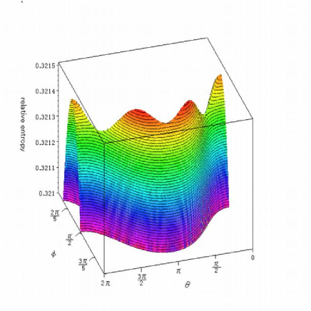
Detailed view of the dark “ridge” near $\phi=\frac{\pi}{2}$ showing 3 distinct maxima and saddle points.

Figure 3: Plots of relative entropy of output states with respect to the optimal average output as a function of a pair of angles defining pure input states on the surface of the Bloch sphere. The edges $\theta=0$ and $\theta=2\pi$ meet on the sphere, so that the figures show two halves of the two maxima with $y=0$, one near the north pole and one on the ridge.

The 4-state channel found in Section 4 is not unique. For example, the channel $\Gamma(\rho(x,y,z))=\linebreak\rho(0.8x+0.22,0.8015y,0.75z+0.245)$ also requires 4-states to optimize capacity. In view of the discussion above it is reasonable to expect that one can find a family of 4-state channels which have the form $\Gamma(\rho(x,y,z))=\rho(\lambda_{1}x+\epsilon_{1},(\lambda_{1}+\epsilon_{2})y,\lambda_{3}z+t_{3})$ with $\epsilon_{k}$ suitable small constants, $\lambda_{3}+t_{3}=1-\epsilon_{3}$, and $\lambda_{1}>\lambda_{3}$ chosen so that $\Gamma(\rho(x,y,z))=\rho(\lambda_{1}x,\lambda_{1}y,\lambda_{3}z+t_{3})$ is close to a 3-state channel.

In the class of channels above, one always has $t_{2}=0$, which raises the question of whether or not there exist 4-state channels exist with all $t_{k}$ all non-zero. Therefore, maps of the form $\Gamma(\rho(x,y,z))=\rho(0.6x+0.021,0.601y+t_{2},0.5z+0.495)$ were considered with $t_{2}\neq 0$. With $t_{2}<0.48$ such maps are completely positive and the channel with with $t_{2}=0.00005$ was shown to require four inputs to achieve capacity.

7 Equivalence to a relative entropy optimization

Reformulation of the capacity optimization in the dual form (2) was also used by Audenaert and Braunstein [1] and by Shirokov [25] to obtain theoretical results and plays an important role in Shor’s proof [27] of equivalence of additivity questions. The implication that the optimal outputs for the capacity then define a supporting hyperplane for the output entropy function $S[\Gamma(\rho)]$ can also be reformulated in terms of relative entropy.

The relative entropy is defined as $H(\omega,\rho)\equiv{\rm Tr}\;\omega(\log\omega-\log\rho)$. It then follows that

$$S(\rho)-\sum_{i}\pi_{i}S(\rho_{i})=\sum_{i}\pi_{i}H(\rho_{i},\rho)$$ (9)

and

$$C(\Gamma)=\sup_{\rho}\sup_{\pi_{i},\rho_{i}}\Big{\{}\sum_{i}\pi_{i}H[\Gamma(\rho_{i}),\Gamma(\rho)]:\textstyle{\sum}_{i}\pi_{i}\rho_{i}=\rho,\pi_{i}>0,\textstyle{\sum}_{i}\pi_{i}=1\Big{\}}.$$ (10)

Moreover, for any fixed $\rho$, and any $\pi_{i},\rho_{i}$

$$\sum_{i}\pi_{i}H[\Gamma(\rho_{i}),\Gamma(\rho)]~{}\leq~{}C(\Gamma)~{}\leq~{}\sup_{\omega}H[\Gamma(\omega),\Gamma(\rho)].$$ (11)

In fact, it was shown in [16] and [24] that

$$C(\Gamma)=\inf_{\rho}\sup_{\omega}H[\Gamma(\omega),\Gamma(\rho)]$$ (12)

from which it follows that when $\rho_{{}^{\rm Av}}$ is the optimal average input, $C(\Gamma)=H[\Gamma(\rho_{i}),\Gamma(\rho_{{}^{\rm Av}})]$ for all $i$. Thus, a necessary condition that an ensemble ${\mathcal{E}}=\{\pi,\rho_{i}\}$ achieve the capacity is that all outputs $\Gamma(\rho_{i})$ are “equidistant” from the average output $\Gamma\big{(}\sum_{i}\pi_{i}\rho_{i}\big{)}$ in the sense that $H[\Gamma(\rho_{i}),\Gamma(\rho_{{}^{\rm Av}})]$ is independent of $i$.

The 4-state optimal ensemble satisfies this requirement, and $H[\Gamma(\rho_{i}),\Gamma(\rho_{{}^{\rm Av}}^{4})]=0.321485159$ for all $i$. If, instead, the 3-state ensemble for the same channel (i.e., the last reported in Table 2) is used, one finds that $H[\Gamma(\rho_{i}^{3}),\Gamma(\rho_{{}^{\rm Av}}^{3})]=0.321460988~{}\forall~{}i$ so that these states also satisfy the equi-distance requirement. However, as one can see from Table 3

$$\sup_{\omega}H[\Gamma(\omega),\Gamma(\rho_{{}^{\rm Av}}^{3})]~{}>~{}0.3215~{}>~{}H[\Gamma(\rho_{i}),\Gamma(\rho_{{}^{\rm Av}}^{3})]$$

showing that the 3-state ensemble is not optimal. Indeed, a plot of $H[\Gamma(\omega),\Gamma(\rho)]$ as shown in Figure 4, shows four relative maxima, which lie closer to the 4-state inputs, than to the 3-state inputs for which $y_{i}=0$. The supremum appears to be achieved for a pair of states with $(x,y,z)=(-0.539291,\pm 0.822613,-0.180202)$. Thus, the relative entropy criterion seems to anticipate the splitting of the input near $(-0.97,0,-0.25)$ into a pair of inputs near $(-0.47,\pm 0.86,-0.17)$.

for images of the two hemispheres of the Bloch sphere.   left: $x>0$    right: $x<0$

Scale:          .

Figure 4: Relative entropy $H[\Gamma(\omega),\Gamma(\rho^{3}_{{}^{\rm Av}})]$ with respect to the 3-state average output $\Gamma(\rho^{3}_{{}^{\rm Av}})$ for image states $\Gamma(\omega)$. Note that this figure is almost indistinguishable from Figure 1. However, the actual locations and values are slightly different as seen by comparing the values in Table 3 below with those in Table LABEL:tab:4st

$$\begin{array}[]{ccc}\omega(x,y,z)&H[\Gamma(\omega),\Gamma(\rho_{{}^{\rm Av}}^{3})]&H[\Gamma(\rho_{i}),\Gamma(\rho_{{}^{\rm Av}}^{3})]\\ (0.252867,0.000000,0.967501)&0.321460988&0.321460986\\ (0.978544,0.000000,0.206036)&0.321460988&0.321460981\\ (-0.539291,0.822613,-0.180202)&0.321505535&0.321504592\\ (-0.539291,-0.822613,-0.180202)&0.321505535&0.321504592\\ \end{array}$$

Table 3: Relative maxima of relative entropy with respect to the 3-state $\rho_{{}^{\rm Av}}^{3}$ for 4-state channel $\Gamma(\rho(x,y,z))=\rho(0.6x+0.021,0.601y,0.5z+0.495)$. The relative entropy for the nearest 4-state input is also given for comparison.

The relative entropy can also be used to check additivity without need to carry out the full variation in (12). In fact, applying (11) to the product channel $\Gamma\otimes\Gamma$ gives

$$2C(\Gamma)\leq C(\Gamma\otimes\Gamma)\leq\sup_{\omega}H\big{[}(\Gamma\otimes\Gamma)(\omega)\,,\,\Gamma(\rho_{{}^{\rm Av}}^{4})\otimes\Gamma(\rho_{{}^{\rm Av}}^{4})\big{]}.$$ (13)

If the supremum on the right equals $2C(\Gamma)$, then the channel is additive. Furthermore, the supremum restricted to product inputs equals $2C(\Gamma)$. Therefore, if the supremum is strictly greater than $2C(\Gamma)$, it must be attained for a pure entangled state $\omega$. But this would imply that the optimal average input is not a product and, hence, that $\Gamma$ is superadditive. Thus, to determine whether or not additivity holds, it is enough to study the supremum in (13) for the product input $\rho_{{}^{\rm Av}}^{4}\otimes\rho_{{}^{\rm Av}}^{4}$; it is not necessary to find the optimal inputs for the product channel.

In order to reformulate the relative entropy optimization in terms of a hyperplane condition, we introduce some notation and review some elementary facts. First, recall that ${\rm Tr}\,A^{\dagger}B=\sum_{jk}\overline{a}_{jk}b_{jk}={\bf\overline{a}}\cdot{\bf b}$ where a, b denote vectors with components $a_{jk}$ and $b_{jk}$ respectively. Alternatively, let $\{M_{k}\}_{k=0,1\ldots d^{2}-1}$ be an orthonormal basis of $d\times d$ matrices with ${\rm Tr}\,M_{j}^{\dagger}M_{k}=\delta_{jk}$ and $M_{0}=\frac{1}{d}I$. Then an arbitrary matrix $A$ can be written as $A=\sum_{k}\alpha_{k}M_{k}$ with $\alpha_{k}={\rm Tr}\,M_{k}^{\dagger}A$, and ${\rm Tr}\,A^{\dagger}B=\sum_{k}\overline{\alpha}_{k}\beta_{k}$. A familiar example of such a basis for $2\times 2$ matrices is $\{\tfrac{1}{2}\sigma_{0},\tfrac{1}{2}\sigma_{1},\tfrac{1}{2}\sigma_{2},\tfrac{1}{2}\sigma_{3}\}$ where $\sigma_{0}$ denotes the identity $I$. An example for $4\times 4$ matrices is $\{\frac{1}{4}\sigma_{k}\sigma_{k}\}_{j,k=0,1,2,3}$ We will be primarily interested in basis and matrices which, like the two examples above, are self-adjoint; therefore, we drop the adjoint symbol $~{}^{\dagger}$ and assume the coefficients $\alpha_{k}$ are real. For a density matrix $\rho$ we will let $\beta(\rho)$ be the vector associated with the trace zero part of $\rho$ so that $\rho=\frac{1}{d}I+\sum_{k}\beta_{k}M_{k}$. Using the Pauli basis for qubits, $\beta(\rho)$ is simply the vector with components $(x,y,z)$ in ${\bf R}^{3}$ associated with the Bloch sphere.

Now let $F(\rho)=S[\Gamma(\rho)]-\xi\cdot\Gamma(\rho)$ with $\xi$ defining a supporting hyperplane for the capacity optimization as discusses in Section 2, and let $G(\rho)=H[\Gamma(\rho),\Gamma(\rho_{{}^{\rm Av}})]$ with $\rho_{{}^{\rm Av}}$ the optimal average. Writing $\log\Gamma(\rho_{{}^{\rm Av}}))=\sum_{k}\tau_{k}M_{k}$, one finds

$$G(\rho)=H[\Gamma(\rho),\Gamma(\rho_{{}^{\rm Av}})] = -S[\Gamma(\rho)]-{\rm Tr}\,\Gamma(\rho)\,\log(\Gamma(\rho_{{}^{\rm Av}}))$$ (14)

$$= -S[\Gamma(\rho)]-\tau_{0}-\tau\cdot\beta(\Gamma(\rho)).$$

Therefore, $H[\Gamma(\rho),\Gamma(\rho_{{}^{\rm Av}})]+S[\Gamma(\rho)]$ defines a hyperplane and $G(\rho)+\tau_{0}\leq C(\Gamma)$ holds with equality for the optimal inputs $\rho_{i}$. This implies that the supporting hyperplane condition $F(\rho)\geq A$ holds with equality for optimal inputs $\rho_{i}$ when $\xi=-\tau$. In that case, $F(\rho)=-G(\rho)-\tau_{0}$ and $A=\tau_{0}-C(\Gamma)$. With $d+1$ optimal inputs, the supporting hyperplane is the unique hyperplane given by the relative entropy.

For the 4-state channel $\xi=(0.039662,0,0.962107)$ and we see from Table 1 that $A=0.978506$ and $B=0.321485$. A computation gives $\log(\Gamma(\rho_{{}^{\rm Av}}))=1.299989I+0.039662\sigma_{x}+0.962105\sigma z$, from which it follows immediately that $\tau=-\xi$ and $F(\rho)=1.299989-G(\rho)$ as expected.

8 Additivity

As mentioned earlier, 4-state channels might be good candidates for examining the additivity of channel capacity. Those considered here have the property $\lambda_{2}>\max_{i=1,3}|\lambda_{i}|$, $t_{2}=0$ and $t_{1},t_{3}\neq 0$. Channels of this type do not belong to one of the classes of qubit maps for which multiplicativity of the maximal p-norm has been proved and its geometry seems resistant to simple analysis. (See [10] for a summary and further references.) Because one state lies very close the the Bloch sphere, with all others much further away, one expects that additivity of minimal entropy and multiplicativity of the maximal p-norm surely hold for this channel. Nevertheless, this has not been proven, suggesting that the channel may have subtle properties. Indeed, most known proofs of additivity for minimal entropy for a particular class of channels, also yield additivity of channel capacity for the same class. These conjectures are now known to be equivalent [27], but this equivalence requires the use of non-trivial channel extensions and does not hold for individual channels. Thus the resistance to proof of of a seemingly obvious fact using current techniques may indicate that the far less obvious additivity of channel capacity does not hold.

We will use the fact that $\Gamma$ is additive if $\sup_{\omega}G(\omega)=2C(\Gamma)$, but superadditive if $G(\omega)>2C(\Gamma)$ for some state $\omega$ where $G(\omega)=H\big{[}(\Gamma\otimes\Gamma)(\omega)\,,\,\Gamma(\rho_{{}^{\rm Av}}^{4})\otimes\Gamma(\rho_{{}^{\rm Av}}^{4})\big{]}.$ The function $g(\rho)=H[\Gamma(\rho),\Gamma(\rho_{{}^{\rm Av}}^{4})]$ has 10 critical points(4 maxima, 4 saddle points, and 2 (relative) minima), as shown in Figure 3. This implies that $G(\omega)$ has at least 100 critical points, 16 maxima, 4 (relative) minima, and 80 saddle-like critical points when one restricts $\omega$ to a product state. The complexity of this landscape seems greater than that of any other class of channels studied. If the capacity of any qubit channel is non-additive, it seems likely that it would be a channel of this type. Therefore, a thorough numerical analysis is called for. Unfortunately, the large number of critical points, also make a full optimization very challenging.

It suffices to optimize over pure states of the form $\omega=|\Psi\rangle\langle\Psi|$ with

$$|\Psi\rangle=\sqrt{p}\begin{pmatrix}~{}~{}\cos\theta_{u}\\ e^{i\phi_{u}}\sin\theta_{u}\end{pmatrix}\otimes\begin{pmatrix}~{}~{}\cos\theta_{v}\\ e^{i\phi_{v}}\sin\theta_{v}\end{pmatrix}+e^{i\nu}\sqrt{1-p}\begin{pmatrix}e^{-i\phi_{u}}\sin\theta_{u}\\ ~{}~{}-\cos\theta_{u}\end{pmatrix}\otimes\begin{pmatrix}e^{-i\phi_{v}}\sin\theta_{v}\\ ~{}~{}-\cos\theta_{v}\end{pmatrix}$$ (15)

and $p\in[0,1],~{}\theta_{u},\,\theta_{v},\,\nu\in[0,2\pi],~{}\phi_{u},\,\phi_{v}\in[0,\frac{\pi}{2}]$. To see why this is true, note that (15) says that $|\Psi\rangle=\sqrt{p}\,|u\rangle\otimes|v\rangle+e^{i\nu}\sqrt{1-p}\,|u^{\perp}\rangle\otimes|v^{\perp}\rangle$ where $|u^{\perp}\rangle$ denotes the vector orthogonal to $|u\rangle=\begin{pmatrix}~{}~{}\cos\theta\\ e^{i\phi}\sin\theta\end{pmatrix}$. Note that

$$|u\rangle\langle u|=\tfrac{1}{2}\big{[}I+\sin 2\theta\,\cos\phi\,\sigma_{x}+\sin 2\theta\,\sin\phi\,\sigma_{y}+\cos 2\theta\,\sigma_{z}\big{]}~{}.$$

Now let $\gamma_{u}=\Gamma(|u\rangle\langle u|)$. Then we can write

$$(\Gamma\otimes\Gamma)(|\Psi\rangle\langle\Psi|)=p\,\gamma_{u}\otimes\gamma_{v}+(1-p)\,\gamma_{u^{\perp}}\!\otimes\gamma_{v^{\perp}}+\sqrt{p(1-p)}\,X$$ (16)

where

$$X=e^{-i\nu}\Gamma(|u\rangle\langle u^{\perp}|)\otimes\Gamma(|v\rangle\langle v^{\perp}|)+e^{i\nu}\Gamma(|u^{\perp}\rangle\langle u|)\otimes\Gamma(|v^{\perp}\rangle\langle v|)$$

Since ${\rm Tr}\,|u\rangle\langle u^{\perp}|=\langle u^{\perp}|u\rangle=0$ and $\Gamma$ is trace-preserving, the partial traces of $X$ are zero, i.e.

$${\rm Tr}_{1}\,X={\rm Tr}_{2}\,X=0~{}.$$ (17)

It then follows immediately that ${\rm Tr}\,X\,\log\varrho_{1}\otimes\varrho_{2}=0$ since

$${\rm Tr}\,X\,I_{1}\otimes\log\varrho_{2}+{\rm Tr}\,X\,(\log\varrho_{1})\otimes I_{2}={\rm Tr}_{2}\big{[}\log\varrho_{2}({\rm Tr}_{1}\,X)\big{]}+{\rm Tr}_{1}\,\big{[}\log\varrho_{1}({\rm Tr}_{2}X)\big{]}=0$$ (18)

Applying this with $\varrho=\Gamma(\rho_{{}^{\rm Av}}^{4})$ one finds that

$${\rm Tr}\,(\Gamma\otimes\Gamma)(|\Psi\rangle\langle\Psi|)\,\log\Gamma(\rho_{{}^{\rm Av}}^{4})\otimes\Gamma(\rho_{{}^{\rm Av}}^{4})=0$$ (19)

Therefore the second term in the relative entropy is affine in $p$. Hence any non-linearity in $H(\Gamma\otimes\Gamma)(|\Psi\rangle\langle\Psi|),\Gamma(\rho_{{}^{\rm Av}}^{4})\otimes\Gamma(\rho_{{}^{\rm Av}}^{4})$ must come entirely from the entropy term $-S\big{[}(\Gamma\otimes\Gamma)(|\Psi\rangle\langle\Psi|)\big{]}$.

Because of the difficulty of optimizing over all six parameters, plots of $G(\omega)$ were made as a function of only $p,\nu$ with $u,v$ fixed and as a function of $p$ with the remaining 5 parameters fixed. A typical example is shown in Figure 5 and appears to be convex function in $p$ for several choices of $nu$. Many other examples were considered with $u,v$ both corresponding to optimal inputs, $u,v$ chosen randomly, $u,v$ chosen to be highly non-optimal, and various combinations of these. The shape of the curve seems to be extremely resilient for all inputs in Schmidt form (15) and suggests convexity in $p$ with a deep minimum. Although the minimum lies above that for the corresponding mixed state with $X=0$, it is well below both endpoints. Changes as $\nu$ ranges from $0$ to $2\pi$ are small.

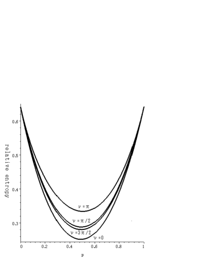
Figure 5: Typical plot of $G(\omega)=H\big{[}(\Phi\otimes\Phi)(\omega),\Phi(\rho_{{}^{\rm Av}})\otimes\Phi(\rho_{{}^{\rm Av}})\big{]}$ as of function of $p$ for $\nu=0,\frac{\pi}{2},\pi,\frac{3\pi}{2}$ using pure states of the form (15) and $u,v$ fixed and $e^{i\nu}=1,i,-i,-1$. Endpoints correspond to product states and $p=0.5$ maximally entangled .

States of the form $\frac{1}{\sqrt{2}}\big{(}|u_{i}\rangle\otimes|u_{j}\rangle+e^{i\nu}|u_{k}\rangle\otimes|u_{\ell}\rangle\big{)}$ with $u_{i}$ corresponding to the four optimal inputs were also considered. Because these $u_{i}$ are not orthogonal, the functions do not have the form (15) and (19) need not hold. Although the relative entropy has a slightly different shape as a function of $p$ and $\nu$, it still lies below the plane $2C(\Gamma)$ and has a deep minimum.

Thus, there seems to be little room for obtaining a counter-example by varying the channel parameters. This may give the strongest numerical evidence for additivity yet, at least in the case of qubit channels.

Remark: Because the second term in the relative entropy is affine in $p$ for states of the form (15), the concavity of the entropy function $g_{u,v,\nu}(p)\equiv S\big{[}(\Gamma\otimes\Gamma)(|\Psi\rangle\langle\Psi|)\big{]}$ as a function of $p$ for arbitrary states of the form form (15). This would immediately yield both additivity of minimal entropy and of channel capacity. It is very tempting to conjecture that $g_{u,v,\nu}(p)$ is concave.

A similar conjecture was made independently in [3] with supporting evidence for a particular set of channels with $d>3$. Despite the appeal of this conjecture, it is false. Consider the channels $\Gamma[\rho(x,y,z)]=\rho(\mu x,\mu y,0.5x)$ with $0\leq\mu\leq 0.75$ and $|\psi\rangle=\sqrt{p}|00\rangle+\sqrt{1-p}|11\rangle$. Then $\Gamma\otimes\Gamma)\big{(}|\psi\rangle\langle\psi|\big{)}$ has eigenvalues $\frac{3}{16},\frac{3}{16},\frac{5\pm 4\sqrt{1+(16\mu^{4}-4)p(1-p)}}{16}$. It follows that $f(p)=S\big{[}(\Gamma\otimes\Gamma)\big{(}|\psi\rangle\langle\psi|\big{)}\big{]}$ is concave for $\mu\leq\frac{1}{\sqrt{2}}$ and convex for $\mu\geq\frac{1}{\sqrt{2}}$ as shown in Figure 6. This example above also implies that a related conjecture [3] for Schur concavity is false. Note however, that the chosen inputs are not optimal when $\mu>\frac{1}{2}$ and far from optimal when $\mu>\frac{1}{\sqrt{2}}$; indeed even the lowest point on convex curve shown lies well above the true minimal output entropy of 1.2017521 for $\mu=\frac{1}{\sqrt{2}}$ and 1.087129 for $\mu=0.75$.

If products of the optimal inputs $\frac{1}{\sqrt{2}}(|0\rangle\pm|1\rangle)$ are entangled, the corresponding entropy function is known [9] to be concave. Moreover, King has [8] shown that both the minimal entropy and the capacity are additive for these channels for all $\mu$.

It seems likely that the conjectured concavity holds when optimal inputs are entangled; however, this is not sufficient to prove additivity of either capacity or minimal entropy.

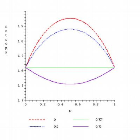
Figure 6: Plots of $f(p)=S\big{[}(\Gamma\otimes\Gamma)\big{(}|\psi\rangle\langle\psi|\big{)}\big{]}$ for $\mu=0,0.5,0.707,0.75$ with $\Gamma[\rho(x,y,z)]=\rho(\mu x,\mu y,0.5x)$ and $|\psi\rangle=\sqrt{p}\,|00\rangle+\sqrt{1-p}\,|11\rangle$. The top curve with $\mu=0$ reduces to the usual concavity of the mixed state $(\Gamma\otimes\Gamma)(p|00\rangle\langle 00|+(1-p)|11\rangle\langle 11|$; the next with $\mu=0.5$ shows the expected concavity; the flat horizontal curve is for $\mu=0.707$, or $\sqrt{2}$; the bottom curve shows $\mu=0.75$ for which the inputs are no longer optimal and $f_{\mu}(p)$ is convex.

Acknowledgment

The authors would like to thank Dr. Mitsuru Hamada for his useful comments on this problem. This work was begun when M.B.R. visited the ERATO in September, 2003, and some of the work of T.S. was done during a visit to Tufts University in February, 2004.

References

- [1] K. M. R. Audenaert and S. L. Braunstein, “On strong superadditivity of the entanglement of formation”, Commun. Math. Phys. 246, 443–452 (2004).
- [2] E. B. Davies, “Information and Quantum Measurements” IEEE Trans. Inf. Theory 24, 596–599 (1978).
- [3] N. Datta, A. S.Holevo, Y. M.Suhov, “A quantum channel with additive minimum output entropy” quant-ph/0403072
- [4] A. Fujiwara and P. Algoet, “One-to-one parametrization of quantum channels” Phys. Rev. A 59, 3290–3294 (1999).
- [5] A. Fujiwara and H. Nagaoka, “Operational Capacity and Pseudoclassicality of a Quantum Channel” IEEE Trans. Inf. Theory , 44, 1071–1086 (1988).
- [6] A. S. Holevo “The Capacity of the Quantum Channel with General Signal States IEEE Trans. Inf. Theory 44, 269–273 (1998).
- [7] H. Imai, M. Hachimori, M. Hamada, H. Kobayashi and K. Matsumoto:, “Optimization in Quantum Computation and Information” Proceedings of the 2nd Japanese-Hungarian Symposium on Discrete Mathematics and Its Applications, pp.60–69 (Budapest, April 2001) .
- [8] C. King, “Additivity for unital qubit channels” J. Math. Phys. 43, 4641–4653 (2004).
- [9] C. King and M. B. Ruskai, “Minimal Entropy of States Emerging from Noisy Quantum Channels” IEEE Trans. Info. Theory 47, 192–209 (2001).
- [10] C. King and M. B. Ruskai, “Comments on Multiplicativity of p-norms for p = 2” in Quantum Information, Statistics and Probability ed. by O. Hirota, in press (World Scientific, 2004); quant-ph/0401026
- [11] C. King, M. Nathanson and M. B. Ruskai: Qubit Channels can Require More Than Two Inputs to Achieve Capacity. Phys. Rev. Lett., 88, 057901 (2002).
- [12] C. Macchiavello, G. M. Palma, S. Virmani “Transition behavior in the channel capacity of two-quibit channels with memory” Phys. Rev. A 69, 010303 (2004) .
- [13] K. Matsumoto, T. Shimono, A. Winter: “Remarks on additivity of the Holevo channel capacity and of the entanglement of formation”, Commun. Math. Phys. 246, 427–442 (2004).
- [14] Mathematical Systems Inc.: NUOPT. http://www.msi.co.jp/en/home.html.
- [15] H. Nagaoka “Algorithms of Arimoto-Blahut Type for Computing Quantum Channel Capacity” Proc. 1998 IEEE International Symposium on Information Theory, p.354 (1998).
- [16] M. Ohya, D. Petz and N. Watanabe, “On capacities of quantum channels” Prob. Math. Stats. 17, 170–196 (1997).
- [17] S. Osawa and H. Nagaoka, “Numerical Experiments on the Capacity of Quantum Channel with Entangled Input States” IEICE Trans. Fundamentals, E84-A, 2583–2590 (October 2001)
- [18] A. A. Pomeransky, “Strong superadditivity of the entanglement of formation follows from its additivity” Phys. Rev. A, 68, 032317 (2003). quant-ph/0305056
- [19] F. Potra and Y. Ye, “A Quadratically Convergent Polynomial Algorithm for Solving Entropy Optimization Problems” SIAM J. Optim., 3 843–860 (1993).
- [20] R. T. Rockafellar, Convex Analysis (Princeton University Press, 1970).
- [21] M. B. Ruskai, “Qubit Entanglement Breaking Channels” Reviews in Mathematical Physics, 15, 643–662 (2003).
- [22] M. B. Ruskai, S. Szarek and E. Werner, “An Analysis of Completely-Positive Trace-Preserving maps on ” Linear Algebra and its Applications, 347, 159–187 (2002).
- [23] B. Schumacher and M. D. Westmoreland “Sending Classical Information via Noisy Quantum Channels” Phys. Rev. A, 56, 131–138 (1997).
- [24] B. Schumacher and M. D. Westmoreland “Optimal signal ensembles” Phys. Rev. A 63, 022308 (2001).
- [25] M.E. Shirokov, “On the structure of optimal sets for tensor product channels” quant-ph/0402178
- [26] P. W. Shor: Capacities of Quantum Channels and How to Find Them. Math. Program. (ISMP 2003, Copenhagen), Ser. B, 97, 311–335 (2003), .
- [27] P. W. Shor, “Equivalence of Additivity Questions in Quantum Information Theory”, Commun. Math. Phys. 246, 453–472 (2004).