Generalizing Tsirelson’s bound on Bell inequalities using a min-max principle

Abstract

Bounds on the norm of quantum operators associated with classical Bell-type inequalities can be derived from their maximal eigenvalues. This quantitative method enables detailed predictions of the maximal violations of Bell-type inequalities.

The violations of Bell-type inequalities represent a cornerstone of our present understanding of quantum probability theory Peres (1993). Thereby, the usual procedure is as follows: First, the (in)equalities bounding the classical probabilities and expectations are derived systematically; e.g., by enumerating all conceivable classical possibilities and their associated two-valued measures. These form the extreme points which span the classical correlation polytopes Cirel’son (1980); Tsirelson (1993); Froissart (1981); Pitowsky (1986, 1989a, 1989b, 1991, 1994); Pitowsky and Svozil (2001); Colins and Gisin (2003); Sliwa (2003); the faces of which are expressed by Bell-type inequalities which characterize the bounds of the classical probabilities and expectations; in Boole’s term Boole (1958, 1862), the “conditions of possible experience.” (Generating functions are another method to find bounds on classical expectations Werner and Wolf (2001); Schachner (2003).) The Bell-type inequalities contain sums of (joint) probabilities and expectations. In a second step, the classical probabilities and expectations in the Bell-type inequalities are substituted by quantum probabilities and expectations. The resulting operators violate the classical bounds. Until recently, little was known about the fine structure of the violations. Tsirelson (also written Cirel’son) published an absolute bound for the violation of a particular Bell-type inequality, the Clauser-Horne-Shimony-Holt (CHSH) inequality Cirel’son (1980); Tsirel’son (1987); Tsirelson (1993); Khalfin and Tsirelson (1992). Cabello has investigated a violation of the CHSH inequality beyond the quantum mechanical bound by applying selection schemes to particles in a GHZ-state Cabello (2002a, b). Recently, detailed numerical Filipp and Svozil (2004) and analytical studies Cabello (2004) stimulated experiments Bovino et al. (2004) to test the quantum bounds of certain Bell-type inequalities.

In what follows, a general method to compute quantum bounds on Bell-type inequalities will be reviewed systematically. It makes use of the min-max principle for self-adjoint transformations (Ref. Halmos (1974), Sec. 90 and Ref. Reed and Simon (1978), Sec. 75) stating that the operator norm is bounded by the minimal and maximal eigenvalues. These ideas are not entirely new and have been mentioned previously Werner and Wolf (2001); Filipp and Svozil (2004); Cabello (2004), yet to our knowledge no systematic investigation has been undertaken yet. It should also be kept in mind that this method a priori cannot produce quantum polytopes Pitowsky (2002); Filipp and Svozil (2004), but the quantum correspondents of classical polytopes. Indeed, as we demonstrate explicitly, the resulting geometric forms are not convex. This, however, does not diminish the relevance of these quantum predictions to experiments testing the quantum violations of classical Bell-type inequalities.

As a starting point note that since $(A+B)^{\dagger}=A^{\dagger}+B^{\dagger}=(A+B)$ for arbitrary self-adjoint transformations $A,B$, the sum of self-adjoint transformations is again self-adjoint. That is, all self-adjoint transformations entering the quantum correspondent of any Bell-type inequality is again a self-adjoint transformation. The sum does not preserve eigenvectors and eigenvalues; i.e., $A+B$ can have different eigenvectors and eigenvalues than $A$ and $B$ taken separately (i.e., $A$ and $B$ need not necessarily commute). The norm of the self-adjoint transformation resulting from summing the quantum counterparts of all the classical terms contributing to a particular Bell inequality obeys the min-max principle. Thus determining the maximal violations of classical Bell inequalities amounts to solving an eigenvalue problem. The associated eigenstates are the multi-partite states which yield a maximum violation of the classical bounds under the given experimental (parameter) setup .

Let us demonstrate the method by considering two particles propagating in inverse directions; their polarization or spin being measured along two and more ($m$) distinct directions per particle perpendicular to their propagation directions. For these configurations, we shall enumerate analytical quantum bounds corresponding to the Clauser-Horne (CH) inequality, as well as of more general inequalities for $m>2$ Pitowsky and Svozil (2001); Colins and Gisin (2003); Sliwa (2003).

For $m=2$, the CH inequalities restrict classical probabilities by $-1\leq p_{13}+p_{14}+p_{23}-p_{24}-p_{1}-p_{3}\leq 0$, as well as permutations thereof. Here, $p_{1}$ and $p_{3}$ stand for the probabilities that the first particle is measured along the first direction and the second particle is measured along the third direction. $p_{ij}$ stands for the joint probability to find the first particle along the direction $i$ and the second particle along the direction $j$.

In order to evaluate the quantum counterpart of the CH inequalities, the classical probabilities have to be substituted by the quantum ones; i.e.,

$$\begin{array}[]{lll}p_{1}&\rightarrow&q_{1}(\theta)={\frac{1}{2}}\left[{\mathbb{I}}_{2}+{\bf\sigma}(\theta)\right]\otimes{\mathbb{I}}_{2},\\ p_{3}&\rightarrow&q_{3}(\theta)={\mathbb{I}}_{2}\otimes{\frac{1}{2}}\left[{\mathbb{I}}_{2}+{\bf\sigma}(\theta)\right],\\ p_{ij}&\rightarrow&q_{ij}(\theta,\theta^{\prime})={\frac{1}{2}}\left[{\mathbb{I}}_{2}+{\bf\sigma}(\theta)\right]\otimes{\frac{1}{2}}\left[{\mathbb{I}}_{2}+{\bf\sigma}(\theta^{\prime})\right],\end{array}$$ (1)

with ${\bf\sigma}(\theta)=\begin{pmatrix}\cos\theta&\sin\theta\\ \sin\theta&-\cos\theta\end{pmatrix}$, where $\theta$ is the relative measurement angle in the $x$–$z$-plane, and the two particles propagate along the $y$-axis. The quantum transformation associated with the CH inequality enumerated above is thus given by

$$\begin{array}[]{lcl}O_{22}(\alpha,\beta,\gamma,\delta)&=&q_{13}(\alpha,\gamma)+q_{14}(\alpha,\delta)+q_{23}(\beta,\gamma)-q_{24}(\beta,\delta)-q_{1}(\alpha)-q_{3}(\gamma)\\ &=&{\frac{1}{2}}\left[{\mathbb{I}}_{2}+{\bf\sigma}(\alpha)\right]\otimes{\frac{1}{2}}\left[{\mathbb{I}}_{2}+{\bf\sigma}(\gamma)\right]+{\frac{1}{2}}\left[{\mathbb{I}}_{2}+{\bf\sigma}(\alpha)\right]\otimes{\frac{1}{2}}\left[{\mathbb{I}}_{2}+{\bf\sigma}(\delta)\right]\\ &&+{\frac{1}{2}}\left[{\mathbb{I}}_{2}+{\bf\sigma}(\beta)\right]\otimes{\frac{1}{2}}\left[{\mathbb{I}}_{2}+{\bf\sigma}(\gamma)\right]-{\frac{1}{2}}\left[{\mathbb{I}}_{2}+{\bf\sigma}(\beta)\right]\otimes{\frac{1}{2}}\left[{\mathbb{I}}_{2}+{\bf\sigma}(\delta)\right]\\ &&-{\frac{1}{2}}\left[{\mathbb{I}}_{2}+{\bf\sigma}(\alpha)\right]\otimes{\mathbb{I}}_{2}-{\mathbb{I}}_{2}\otimes{\frac{1}{2}}\left[{\mathbb{I}}_{2}+{\bf\sigma}(\gamma)\right],\end{array}$$ (2)

where $\alpha$, $\beta$, $\gamma$, $\delta$ denote the measurement angles lying in the $x$–$z$-plane: $\alpha$ and $\beta$ for one particle, $\gamma$ and $\delta$ for the other one. The eigenvalues of the self-adjoint transformation in (2) are

$$\lambda_{1,2,3,4}(\alpha,\beta,\gamma,\delta)=\frac{1}{2}\big{(}\pm\sqrt{1\pm\sin(\alpha-\beta)\sin(\gamma-\delta)}-1\big{)}$$ (3)

yielding the maximum bound $\|O_{22}\|=\max_{i=1,2,3,4}\lambda_{i}$. Note that for the particular choice of parameters $\alpha=0,\beta=2\theta,\gamma=\theta,\delta=3\theta$ adopted in Cabello (2004); Filipp and Svozil (2004), one obtains $|O_{22}|=\frac{1}{2}\left\{\left[\left(3-\cos 4\theta\right)/2\right]^{1/2}-1\right\}$.

In the Bell-basis $\{|\phi^{+}\rangle,|\psi^{+}\rangle,|\psi^{-}\rangle,|\phi^{-}\rangle\}$ with $|\psi^{\pm}\rangle=1/\sqrt{2}(|01\rangle\pm|10\rangle)$ and $|\phi^{\pm}\rangle=1/\sqrt{2}(|00\rangle\pm|11\rangle)$, the eigenvectors corresponding to the maximal violating eigenstates are

$$\begin{array}[]{ccl}|\nu_{\pm}\rangle&=&\big{(}F^{\pm}(\alpha,\beta,-\gamma,-\delta)|\psi^{+}\rangle+|\phi^{-}\rangle\big{)}\big{(}1+F^{\pm}(\alpha,\beta,-\gamma,-\delta)^{2}\big{)}^{-\frac{1}{2}},\\ |\mu_{\pm}\rangle&=&\big{(}F^{\pm}(\alpha,\beta,\gamma,\delta)|\phi^{+}\rangle+|\psi^{-}\rangle\big{)}\big{(}1+F^{\pm}(\alpha,\beta,\gamma,\delta)^{2}\big{)}^{-\frac{1}{2}},\end{array}$$ (4)

with

$$F^{\pm}(\alpha,\beta,\gamma,\delta)=\pm 2\sqrt{1-\sin(\alpha-\beta)\sin(\gamma-\delta)}\;\;\frac{\cos(\alpha-\delta)-\cos(\alpha-\gamma)-\cos(\beta-\gamma)-\cos(\beta-\delta)}{\sin(\alpha-\gamma)+\sin(\beta-\gamma)-\sin(\alpha-\delta)+\sin(\beta-\delta)}.$$

The states (4) are maximally entangled, corroborating the approach of Cabello Cabello (2004) to utilize a set of maximally entangled states to reconstruct the quantum bound for the setting of the relative angles $\alpha=0$, $\beta=2\theta$, $\gamma=\theta$ and $\delta=3\theta$ . ¿From the particular form of the eigenstates, we conclude that the maximal violating eigenstates of the $O_{22}$ operator are maximally entangled for general measurement angles lying in the $x$–$z$-plane.

Generalizations for $m$ measurements per particle are straightforward; for example, the extension to three measurement operators for each particle yields only one additional nonequivalent (with respect to symmetries) inequality Colins and Gisin (2003); Sliwa (2003) $I_{33}=p_{14}+p_{15}+p_{16}+p_{24}+p_{25}-p_{26}+p_{34}-p_{35}-p_{1}-2p_{4}-p_{5}\leq 0$ among the 684 inequalities Pitowsky and Svozil (2001) representing the faces of the associated classical correlation polytope. The associated operator for symmetric measurement directions is given by

$$\begin{array}[]{lll}&O_{33}(0,\theta,2\theta,0,\theta,2\theta)=q_{14}(0,0)+q_{15}(0,\theta)+q_{16}(0,2\theta)+q_{24}(\theta,0)+q_{25}(\theta,\theta)-q_{26}(\theta,2\theta)+\\ &\qquad+q_{34}(2\theta,\theta)-q_{35}(2\theta,\theta)-q_{1}(0)-2q_{4}(0)-q_{5}(\theta)\\ &\qquad\qquad=\frac{1}{4}\left(\begin{smallmatrix}-4\sin^{2}\theta&0&0&0\\ 0&-5-2\cos\theta-3\cos 2\theta+2\cos 3\theta&4\cos^{2}\frac{\theta}{2}&2\sin\theta+3\sin 2\theta-2\sin 3\theta\\ 0&4\cos^{2}\frac{\theta}{2}&-2(3+\cos 2\theta)&-2\sin\theta\\ 0&2\sin\theta+3\sin 2\theta-2\sin 3\theta&-2\sin\theta&2\sin^{2}\frac{\theta}{2}\cos^{2}\frac{\theta}{2}(4\cos\theta-3)\end{smallmatrix}\right),\end{array}$$ (5)

again in the Bell basis and for quantum expressions similar to the ones enumerated in Eq. (1) .

In this basis, the operator $O_{33}(0,\theta,2\theta,0,\theta,2\theta)$ splits into a direct sum of a one-dimensional part $-\sin^{2}\theta$ and a three-dimensional part $o$, respectively. Using the Cardano method (see Ref. Cocolicchio and Viggiano (2000)), one can solve the characteristic equation of the three dimensional submatrix $o$ in the lower right corner of $O_{33}$

$$\lambda^{3}+b(\theta)\lambda^{2}+c(\theta)\lambda+d(\theta)=0,$$ (6)

with the coefficients $b=-\text{Tr}\,o,\ c=1/2\Big{(}\text{Tr}\,^{2}o-\text{Tr}\,o^{2}\Big{)},\ d=-\det o$. (For convenience we omit here the dependence on $\theta$.) The (real) eigenvalues can then be written as Cocolicchio and Viggiano (2000)

$$\lambda_{2}=-2\sqrt{|u|}\cos\frac{\xi}{3}-\frac{b}{3}$$

$$\lambda_{3,4}=\sqrt{|u(x)|}\Big{[}\cos\frac{\xi}{3}\pm\sin\frac{\xi}{3}\Big{]}-\frac{b}{3},$$ (7)

with $u=1/9(3c-b^{2})$ and $\cos\xi=\frac{1}{54}\big{(}9bc-2b^{3}-27d\big{)}/\big{(}u\sqrt{|u|}\big{)}$. In Fig. 1, the eigenvalues $\lambda_{2},\lambda_{3},\lambda_{4}$, together with the eigenvalue $\lambda_{1}=-\sin^{2}\theta$ from the one-dimensional part of $O_{33}$, are plotted as functions of the parameter $\theta$ .

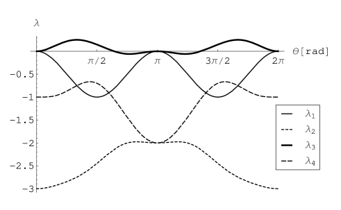
Figure 1: Eigenvalues of $O_{33}$ in dependence of the relative angle $\theta$.

The maximum violation of $1/4$ is obtained for $\theta=\pi/3$ with the associated eigenvector

$$|\Psi_{\rm max}\rangle=\frac{\sqrt{3}}{2}|\phi^{-}\rangle+\frac{1}{2}|\psi^{+}\rangle.$$ (8)

As indicated in Ref. Colins and Gisin (2003), this scheme can be extended to $m$ measurements on each particle by considering inequalities $I_{mm}\leq 0$ and corresponding operators $O_{mm}$ of the form

$$I_{mm} = \sum_{j=1}^{m}\sum_{i=1}^{m-j+1}P({A_{i}B_{j}})-\sum_{i=1}^{m-1}P({A_{i+1}B_{m-i+1}})$$ (9)

$$-\sum_{i=1}^{m}(m-i)P(B_{i})-P(A_{1})\leq 0,$$

where $P(A_{i}B_{j})$ denotes the joint probability of obtaining the value one of the projection operators $A_{i}$ and $B_{j}$ operators on the left and on the right hand side, and $P(A_{i}),\ P(B_{j})$ the marginal probabilities on one side, respectively. For a choice of measurement directions $\{0,\theta,2\theta,\ldots,m\theta\}$ on both sides, the maximizing eigenvalues are plotted in Fig. 2. The matrices belonging to the operators $O_{mm}$ ($m\leq 6$) are of the same form as is $O_{33}$, i. e. they split up into a direct sum of two matrices in the Bell-basis; the maximal eigenvalues can therefore be calculated explicitly using Eqs. (6) and (7).

Figure 2: Maximum violation of the operator $O_{mm}$ for $m=2,\ldots,6$ for a symmetric measurement setup; longer dashes indicate larger $m$.

For experimental realizations of the $O_{33}$ case and special parameter configurations, the ansatz of Cabello Cabello (2004) and Bovino et al. Bovino et al. (2004) can be generalized to arbitrary local unitary transformations $U_{2\times 2}\in SU(2)\otimes SU(2)$ applied to each one of the two particles in some Bell-basis state $|\varphi\rangle$ separately; i.e.,

$$U(\omega_{1},\theta_{1},\phi_{1})\otimes U(\omega_{2},\theta_{2},\phi_{2})|\varphi\rangle.$$ (10)

The single qubit operators are taken as $U(\omega,\theta,\phi)=e^{i\frac{\omega}{2}\vec{n}\cdot\vec{\sigma}}\in SU(2)$ with $\omega$ as the rotation angle about the axis $\vec{n}=(\sin\theta\cos\phi,\sin\theta\sin\phi,\cos\theta)^{T}$. For example, the use of the Bell state $|\psi^{+}\rangle$ and and the successive application of the local unitary operation $U(\omega_{1},\theta_{1},\phi_{1})\otimes U(\omega_{2},\theta_{2},\phi_{2})$ with $\omega_{1}=2\pi/3$, $\theta_{1}=\phi_{1}=\pi/2$ and $\omega_{2}=\theta_{2}=\phi_{2}=0$ yields the maximally violating eigenvector $|\Psi_{\rm max}\rangle$ from Eq. (8) which is also maximally entangled.

For the general $m>2$ case, however, it is not always possible to obtain all possible maximally violating states by starting from a Bell state: for general measurement angles, the experimental realization additionally requires a two-qubit transformation from $SU(4)/(SU(2)\otimes SU(2))$, followed by a local unitary operation $U_{2\times 2}$ in order to obtain all possible states Zhang et al. (2003). As an example, consider the maximally violating but not maximally entangled state at $\theta=\pi/2$: $|\Psi_{\pi/2}\rangle\approx 0.86|\psi^{+}\rangle+0.17|\psi^{-}\rangle+0.47|\phi^{-}\rangle$ cannot be obtained from a Bell state, as entanglement is preserved under $SU(2)\otimes SU(2)$ operations.

Alternatively, multiport interferometry Reck et al. (1994); Zukowski et al. (1997); Svozil (2004) offers a direct proof-of-principle implementation: By choosing the appropriate transmission coefficients and phases in a generalized beam splitter setup, one can prepare any pure state from an input state $|11\rangle\equiv(0,0,0,1)$ corresponding to a photon in a single input port. Take, for example, the maximal eigenstate of the $O_{33}$ operator at $\theta=\pi/2$, $|\Psi_{\pi/2}\rangle\approx 0.86|\psi^{+}\rangle+0.17|\psi^{-}\rangle+0.47|\phi^{-}\rangle\equiv(0.34,0.73,0.49,-0.34)$. The appropriate transmission parameters can be calculated via the identification Reck et al. (1994)

$$\begin{pmatrix}0\\ 0\\ 0\\ 1\end{pmatrix}^{T}R(N)^{-1}=\begin{pmatrix}0.34\\ 0.73\\ 0.49\\ -0.34\end{pmatrix}^{T}=\begin{pmatrix}e^{-i\phi_{1}}\cos\omega_{1}\\ -e^{-i\phi_{2}}\cos\omega_{2}\sin\omega_{1}\\ e^{-i\phi_{3}}\cos\omega_{3}\sin\omega_{2}\sin\omega_{1}\\ -\sin\omega_{3}\sin\omega_{2}\sin\omega_{1}\end{pmatrix}^{T}$$ (11)

for $\omega_{1}=1.23$, $\omega_{2}=2.46$, $\omega_{3}=0.60$ and $\phi_{1}=\phi_{2}=\phi_{3}=0$, where $R(N)$ is a $SU(4)$ rotation serially composed by two-dimensional beamsplitter matrices.

In summary, we have shown how to construct and experimentally test the exact quantum bounds of Bell-type inequalities by solving the eigenvalue problem of the associated self-adjoint transformation. Several problems remain open. Among them is the exact derivation of the quantum correlation hull Pitowsky (2002); Filipp and Svozil (2004), in particular, whether the quantum hull is obtainable by extending the classical Bell-type inequalities in the way as presented above; i.e., by substituting the quantum probabilities for the classical ones. This is by no means trivial, as the sections of the quantum hull need not necessarily be derivable by mere classical extensions. A second open question is related to the geometric structures arising from quantum expectation values. These need not necessarily be convex. Again, the question of direct extensibility remains open for the hull of quantum expectations from the classical ones.

This research has been supported by the Austrian Science Foundation (FWF), Project Nr. F1513. S. F. acknowledges helpful conversations with B. Hiesmayer and S. Scheel.

References

- Peres (1993) A. Peres, Quantum Theory: Concepts and Methods (Kluwer Academic Publishers, Dordrecht, 1993).
- Cirel’son (1980) B. S. Cirel’son (=Tsirel’son), Letters in Mathematical Physics 4, 93 (1980).
- Tsirelson (1993) B. S. Cirel’son (=Tsirel’son), Hadronic Journal Supplement 8, 329 (1993).
- Froissart (1981) M. Froissart, Nuovo Cimento B 64, 241 (1981).
- Pitowsky (1986) I. Pitowsky, J. Math. Phys. 27, 1556 (1986).
- Pitowsky (1989a) I. Pitowsky, Quantum Probability—Quantum Logic (Springer, Berlin, 1989a).
- Pitowsky (1989b) I. Pitowsky, in Bell’s Theorem, Quantum Theory and the Conceptions of the Universe, edited by M. Kafatos (Kluwer, Dordrecht, 1989b), pp. 37–49.
- Pitowsky (1991) I. Pitowsky, Mathematical Programming 50, 395 (1991).
- Pitowsky (1994) I. Pitowsky, Brit. J. Phil. Sci. 45, 95 (1994).
- Pitowsky and Svozil (2001) I. Pitowsky and K. Svozil, Physical Review A 64, 014102 (2001), eprint quant-ph/0011060, URL http://dx.doi.org/10.1103/PhysRevA.64.014102.
- Colins and Gisin (2003) D. Colins and N. Gisin (2003), eprint quant-ph/0306129.
- Sliwa (2003) C. Sliwa, Physics Letters A 317, 165 (2003), eprint quant-ph/0305190, URL http://dx.doi.org/10.1016/S0375-9601(03)01115-0.
- Boole (1958) G. Boole, An investigation of the laws of thought (Dover edition, New York, 1958).
- Boole (1862) G. Boole, Philosophical Transactions of the Royal Society of London 152, 225 (1862).
- Werner and Wolf (2001) R. F. Werner and M. M. Wolf, Phys. Rev. A 64, 032112 (2001), eprint quant-ph/0102024, URL http://dx.doi.org/10.1103/PhysRevA.64.032112.
- Schachner (2003) G. Schachner (2003), eprint quant-ph/0312117.
- Tsirel’son (1987) B. S. Cirel’son (=Tsirel’son), Journal of Soviet Mathematics 36, 557 (1987).
- Khalfin and Tsirelson (1992) L. A. Khalfin and B. S. Tsirelson, Foundations of Physics 22, 879 (1992).
- Cabello (2002a) A. Cabello, Physical Review Letters 88, 060403 (2002a), eprint quant-ph/0108084.
- Cabello (2002b) A. Cabello, Physical Review A 66, 042114 (2002b), eprint quant-ph/0205183.
- Filipp and Svozil (2004) S. Filipp and K. Svozil, Physical Review A 69, 032101 (2004), eprint quant-ph/0306092, URL http://dx.doi.org/10.1103/PhysRevA.69.032101.
- Cabello (2004) A. Cabello, Physical Review Letters 92, 060403 (2004), eprint quant-ph/0309172, URL http://dx.doi.org/10.1103/PhysRevLett.92.060403.
- Bovino et al. (2004) F. A. Bovino, G. Castagnoli, I. P. Degiovanni, and S. Castelletto, Physical Review Letters 92, 060404 (2004), eprint quant-ph/0310042, URL http://dx.doi.org/10.1103/PhysRevLett.92.060404.
- Halmos (1974) P. R. Halmos, Finite-dimensional vector spaces (Springer, New York, Heidelberg, Berlin, 1974).
- Reed and Simon (1978) M. Reed and B. Simon, Methods of Modern Mathematical Physics IV: Analysis of Operators (Academic Press, New York, 1978).
- Pitowsky (2002) I. Pitowsky, in Quantum Theory: Reconsideration of Foundations, Proceedings of the 2001 Växjö Conference (World Scientific, Singapore, 2002), eprint quant-ph/0112068.
- Cocolicchio and Viggiano (2000) D. Cocolicchio and D. Viggiano, J. Phys. A 33, 5669 (2000).
- Zhang et al. (2003) J. Zhang, J. Vala, S. Sastry, and K. B. Whaley, Physical Review A 67, 042313 (2003), URL http://dx.doi.org/10.1103/PhysRevA.67.042313.
- Reck et al. (1994) M. Reck, A. Zeilinger, H. J. Bernstein, and P. Bertani, Physical Review Letters 73, 58 (1994), URL http://dx.doi.org/10.1103/PhysRevLett.73.58.
- Zukowski et al. (1997) M. Zukowski, A. Zeilinger, and M. A. Horne, Physical Review A 55, 2564 (1997), URL http://dx.doi.org/10.1103/PhysRevA.55.2564.
- Svozil (2004) K. Svozil (2004), eprint quant-ph/0401113.
- Braunstein et al. (1992) S. L. Braunstein, A. Mann, and M. Revzen, Physical Review Letters 68, 3259 (1992).
- Mermin (1995) D. N. Mermin, Annals of the New York Academy of Sciences 755, 616 (1995).
- Cereceda (2001) J. L. Cereceda, Foundations of Physics Letters 14, 401 (2001), eprint quant-ph/0101143.