Genuine quantum trajectories for non-Markovian processes

Abstract

A large class of non-Markovian quantum processes in open systems can be formulated through time-local master equations which are not in Lindblad form. It is shown that such processes can be embedded in a Markovian dynamics which involves a time dependent Lindblad generator on an extended state space. If the state space of the open system is given by some Hilbert space ${\mathcal{H}}$, the extended state space is the triple Hilbert space ${\mathcal{H}}\otimes{\mathbb{C}}^{3}$ which is obtained by combining the open system with a three state system. This embedding is used to derive an unraveling for non-Markovian time evolution by means of a stochastic process in the extended state space. The process is defined through a stochastic Schrödinger equation which generates genuine quantum trajectories for the state vector conditioned on a continuous monitoring of an environment. The construction leads to a continuous measurement interpretation for non-Markovian dynamics within the framework of the theory of quantum measurement.

I Introduction

An open quantum system is a certain distinguished quantum system which is coupled to another quantum system, its environment TheWork . A particularly simple way of describing an open system is obtained in the Markovian approximation. In this approximation all memory effects due to system-environment correlations are neglected which usually leads to a Markovian master equation, that is, to a linear first-order differential equation for the reduced density matrix $\rho(t)$ of the open system with a time independent generator. Generally, one demands that the generator is in Lindblad form LINDBLAD , which follows from the requirements of the conservation of probability and of the complete positivity of the dynamical map GORINI1 ; GORINI2 .

A remarkable feature of Markovian master equations in Lindblad form is given by the fact that they allow a stochastic representation, also known as unraveling, by means of a stochastic Schrödinger equation (SSE) for the state vector of the open system CARMICHAEL ; MOLMER ; DUM ; PLENIO ; GISIN . A SSE generates the time evolution of the state vector which results from a continuous monitoring of the environment of the system WISEMAN1 ; WISEMAN2 . A specific realization $\{|\psi(t)\rangle,t\geq 0\}$ of the SSE is called a quantum trajectory: At each time $t\geq 0$ the open system is known to be in a definite state $|\psi(t)\rangle$ under the condition that a specific readout of the monitoring of the system’s environment is given. The reduced density matrix at time $t$ is therefore obtained if one averages the quantity $|\psi(t)\rangle\langle\psi(t)|$ over all possible quantum trajectories. This means that the relation $\rho(t)=E[|\psi(t)\rangle\langle\psi(t)|]$ holds, where the symbol $E$ denotes the ensemble average or expectation value.

In the Markovian case it is thus true that the environment acts as a quantum probe by which an indirect continuous observation of the system is carried out. The description by means of a Markovian master equation in Lindblad form is, however, only an approximation which uses the assumption of short correlation times. For strong couplings and low temperature environments memory effects can lead to pronounced non-Markovian behavior.

It is sometimes argued that the treatment of non-Markovian processes by means of master equations necessarily requires solving integro-differential equations for the reduced density matrix. Such equations arise, for example, in the application of the Nakajima-Zwanzig projection operator technique NAKAJIMA ; ZWANZIG which leads to dynamic equations involving a retarded memory kernel and an integration over the past history of the system.

However, the usage of another variant of the projection operator method allows in many cases the derivation of approximate or even exact non-Markovian master equations for the reduced density matrix which are local in time. This method is known as the time-convolutionless (TCL) projection operator technique SHIBATA1 ; SHIBATA2 ; ROYER1 ; ROYER2 . The non-Markovian character of the TCL master equation is reflected by the fact that its generator may depend explicitly on time and may not be in Lindblad form.

Time-local equations which are of the form of the TCL master equation have also been derived by other means, e. g., by path integral and influence functional techniques FEYNMAN ; CALDEIRA . A well known example is provided by the exact equation of motion for a damped harmonic oscillator coupled linearly to a bosonic reservoir HAAKE ; HU ; KARRLEIN .

The fact that the TCL generator is generally not in Lindblad form leads to several important mathematical and physical consequences. In particular, a stochastic unraveling of the TCL master equation of the form indicated above does not exist: Any such process will automatically produce a master equation whose generator is in Lindblad form. The question is therefore as to whether one can develop a general method for the construction of stochastic Schrödinger equations for non-Markovian dynamics which do have a physical interpretation in terms of continuous measurements. It is the purpose of this paper to show that this is indeed possible.

Our starting point is a time-local non-Markovian master equation for the density matrix $\rho(t)$ on some Hilbert space ${\mathcal{H}}$ with a time dependent and bounded generator. It will be demonstrated that the dynamics given by such a master equation can always be embedded in a Markovian dynamics on an appropriate extended state space. The non-Markovian dynamics thus appears as part of a Markovian evolution in a larger state space.

If one chooses the extended state space as the Hilbert space of the total system, consisting of open system plus environment, this statement is of course trivial. However, it turns out that the embedding can be realized in a fairly simple, much smaller state space, namely in the tensor product space ${\mathcal{H}}\otimes{\mathbb{C}}^{3}$. In physical terms this is the state space of a composite quantum system which results if one combines the original open system on the state space ${\mathcal{H}}$ with a further auxiliary three state system described by the state space ${\mathbb{C}}^{3}$. The open system could be, for example, a damped quantum particle interacting with a dissipative environment. The auxiliary system can then be realized through an additional internal degree of freedom of the particle which leads to a state space spanned by three basis states.

It will be demonstrated that the dynamics in the extended state space follows a Markovian master equation with a time dependent generator in Lindblad form. The application of the standard unraveling of Markovian master equations to the dynamics in the extended state space therefore yields a stochastic unraveling for the non-Markovian dynamics. The resulting SSE generates genuine quantum trajectories which do admit a physical interpretation in terms of a continuous observation carried out on an environment. The construction thus gives rise to a consistent measurement interpretation for non-Markovian evolution in full agreement with the general setting of quantum measurement theory.

The paper is structured as follows. Section II contains a brief review of the continuous measurement theory for Markovian dynamics. Time dependent generators in Lindblad form are introduced in Sec. II.1, and Sec. II.2 treats the corresponding continuous measurement unraveling. The quantum measurement theory for non-Markovian evolution is developed in Sec. III. We introduce time-local non-Markovian master equations in Sec. III.1. The embedding of these equations in a Markovian dynamics is constructed in Sec. III.2, whereas the derivation of the continuous measurement unraveling is given in Sec. III.3. The construction of the SSE and its physical interpretation are illustrated by means of an example in Sec. IV.

A series of interesting stochastic unravelings of non-Markovian quantum dynamics is known in the literature. Section V contains a discussion of our results and of the relations to alternative non-Markovian SSEs, as well as some conclusions.

II Quantum theory of Markovian dynamics

II.1 Time dependent Lindblad generators

We consider a density matrix $W(t)$ on a state space $\widetilde{\mathcal{H}}$ which obeys a master equation of the form:

$$\frac{d}{dt}W(t) = {\mathcal{L}}(t)W(t)$$ (1)

$$\equiv -i\left[H(t),W(t)\right]+\sum_{i}J_{i}(t)W(t)J_{i}^{\dagger}(t)$$

$$-\frac{1}{2}\sum_{i}\big{\{}J_{i}^{\dagger}(t)J_{i}(t),W(t)\big{\}}.$$

The commutator with the Hamiltonian $H(t)$ represents the unitary part of the evolution and the Lindblad operators $J_{i}(t)$ describe the various decay channels of the system. In analogy to the terminology used for classical master equations, the expressions $J_{i}WJ_{i}^{\dagger}$ may be called gain terms, while the expressions $\{J_{i}^{\dagger}J_{i},W\}$, involving an anti-commutator, may be referred to as loss terms.

Both the Hamiltonian $H(t)$ and the operators $J_{i}(t)$ are allowed to depend on time $t$. The generator ${\mathcal{L}}(t)$ of the master equation may thus be explicitly time dependent and does not necessarily lead to a semigroup. We observe, however, that the superoperator ${\mathcal{L}}(t_{0})$ is in Lindblad form LINDBLAD for each fixed $t_{0}\geq 0$. This means that ${\cal{L}}(t_{0})$ is in the form of the generator of a quantum dynamical semigroup. The particular form of the generator derives from the requirements of complete positivity and of the conservation of the trace GORINI1 ; GORINI2 .

Under certain technical conditions which will be assumed to be satisfied here, one concludes that Eq. (1) yields a 2-parameter family of completely positive and trace preserving maps $V(t,s)$ DAVIES ; ALICKI . These maps can be defined with the help of the chronological time-ordering operator $T$ as

$$V(t,s)=T\exp\left[\int_{s}^{t}d\tau{\mathcal{L}}(\tau)\right],\qquad t\geq s\geq 0,$$ (2)

and satisfy

$$V(t,s)V(s,t^{\prime})=V(t,t^{\prime}),\qquad t\geq s\geq t^{\prime}.$$ (3)

In terms of these maps the solution of the master equation (1) at time $t$ can be written as $W(t)=V(t,s)W(s)$, where $t\geq s\geq 0$. Thus, $V(t,s)$ propagates the density matrix at time $s$ to the density matrix at time $t$.

Each $V(t,s)$ maps the space of density matrices into itself. This means that $V(t,s)$ can be applied to any density matrix $W$ to yield another density matrix $V(t,s)W$. The range of definition of the maps $V(t,s)$ is thus the space of all density matrices and is independent of time. Usually, one associates a Markovian master equation with a time independent generator. We slightly generalize this notion and refer to Eq. (1) as a Markovian master equation with a time dependent Lindblad generator ${\mathcal{L}}(t)$.

II.2 Stochastic unraveling and continuous measurement interpretation

As mentioned already in the Introduction the master equation (1) allows a stochastic unraveling through a random process in the state space $\widetilde{\mathcal{H}}$. This means that one can construct a stochastic dynamics for the state vector $|\Phi(t)\rangle$ in $\widetilde{\mathcal{H}}$ which reproduces the density matrix $W(t)$ with the help of the expectation value

$$W(t)=E\big{[}|\Phi(t)\rangle\langle\Phi(t)|\big{]}.$$ (4)

To mathematically formulate this idea one writes a stochastic Schrödinger equation (SSE) for the state vector $|\Phi(t)\rangle$. An appropriate SSE for which the expectation value (4) leads to the master equation (1) is given by

$$d|\Phi(t)\rangle = -iG(|\Phi(t)\rangle)dt$$ (5)

$$+\sum_{i}\left[\frac{J_{i}(t)|\Phi(t)\rangle}{||J_{i}(t)|\Phi(t)\rangle||}-|\Phi(t)\rangle\right]dN_{i}(t),$$

where we have introduced the nonlinear operator

$$G(|\Phi(t)\rangle)\equiv\left[\hat{H}(t)+\frac{i}{2}\sum_{i}||J_{i}(t)|\Phi(t)\rangle||^{2}\right]|\Phi(t)\rangle.$$ (6)

The term $-iG(|\Phi(t)\rangle)dt$ in Eq. (5), which is proportional to the time increment $dt$, expresses the drift of the process. This drift contribution obviously corresponds to the nonlinear Schrödinger-type equation

$$\frac{d}{dt}|\Phi(t)\rangle=-iG(|\Phi(t)\rangle),$$ (7)

whose linear part involves the non-hermitian Hamiltonian

$$\hat{H}(t)=H(t)-\frac{i}{2}\sum_{i}J_{i}^{\dagger}(t)J_{i}(t).$$ (8)

The nonlinear part of the drift ensures that, although $\hat{H}(t)$ is non-hermitian, the norm is conserved under the deterministic time evolution given by Eq. (7).

The second term on the right-hand side of Eq. (5) represents a jump process leading to discontinuous changes of the wave function, known as quantum jumps. These jumps are described here with the help of the Poisson increments $dN_{i}(t)$ which satisfy the relations:

$$dN_{i}(t)dN_{j}(t) = \delta_{ij}dN_{i}(t),$$ (9)

$$E[dN_{i}(t)] = ||J_{i}(t)|\Phi(t)\rangle||^{2}dt.$$ (10)

According to Eq. (9) the increments $dN_{i}(t)$ are random numbers which take the possible values $0$ or $1$. Moreover, if $dN_{i}(t)=0$ for a particular $i$, we have $dN_{j}(t)=0$ for all $j\neq i$. The state vector then performs the jump

$$|\Phi(t)\rangle\longrightarrow\frac{J_{i}(t)|\Phi(t)\rangle}{||J_{i}(t)|\Phi(t)\rangle||}.$$ (11)

Thus we see that $N_{i}(t)$ is an integer-valued process which counts the number of jumps of type $i$.

We infer from Eq. (10) that $dN_{i}(t)=1$ occurs with probability $||J_{i}(t)|\Phi(t)\rangle||^{2}dt$. The jump described by (11) thus takes place at a rate of $||J_{i}(t)|\Phi(t)\rangle||^{2}$. The case $dN_{i}(t)=0$ for all $i$ is realized with probability $1-\sum_{i}||J_{i}(t)|\Phi(t)\rangle||^{2}dt$. In this case the state vector $|\Phi(t)\rangle$ follows the deterministic drift described by Eq. (7).

Summarizing, the dynamics described by Eq. (5) yields a piecewise deterministic process, i. e., a random process whose realizations consist of deterministic evolution periods interrupted by discontinuous quantum jumps. Since both the deterministic drift (7) as well as the jumps (11) do not change the norm, the whole process preserves the norm of the state vector.

The formulation of the dynamics by means of a SSE bears several numerical advantages over the integration of the corresponding density matrix equation (1). This fact was the original motivation for the development of stochastic wave function methods in atomic physics and quantum optics (for an example, see MOLMER2 ). What is important in our context is the fact that, additionally, the stochastic process given by the SSE allows a physical interpretation in terms of a continuous measurement which is carried out on an environment of the system.

To explain this point we consider a microscopic model in which the open system is weakly coupled to a number of independent reservoirs $R_{i}$, one reservoir for each value of the index $i$. Each reservoir $R_{i}$ consists of bosonic modes $b_{i\lambda}$ which satisfy the commutation relations:

$$\big{[}b_{i\lambda},b^{\dagger}_{j\mu}\big{]}=\delta_{ij}\delta_{\lambda\mu}.$$ (12)

The Lindblad operators $J_{i}(t)$ appearing in the master equation (1) couple linearly to the reservoir operators

$$B_{i}(t)=\sum_{\lambda}g_{i\lambda}e^{i(\omega_{i}-\omega_{i\lambda})t}b_{i\lambda},$$ (13)

where the $\omega_{i}$ are certain system frequencies, $\omega_{i\lambda}$ is the frequency of the mode $b_{i\lambda}$ of reservoir $R_{i}$, and the $g_{i\lambda}$ are coupling constants. Thus, the Hamiltonian of our model is taken to be:

$$H_{I}(t)=H(t)+\frac{1}{\sqrt{\Gamma}}\sum_{i}\left[J_{i}(t)B^{\dagger}_{i}(t)+J^{\dagger}_{i}(t)B_{i}(t)\right].$$ (14)

We have included a factor $1/\sqrt{\Gamma}$, where $\Gamma$ is a typical relaxation rate of the system which will be introduced below. The combination $J_{i}/\sqrt{\Gamma}$ is therefore dimensionless and the $B_{i}$ have the dimension of an inverse time, choosing units such that $\hbar=1$.

The time evolution operator over the time interval $(t,t^{\prime})$ will be denoted by $U(t^{\prime},t)$. The correlation function of reservoir $R_{i}$ can be expressed through the spectral density $I(\omega)$, which is assumed to be the same for all reservoirs:

$$\langle 0|B_{i}(t^{\prime})B_{i}^{\dagger}(t)|0\rangle=\int d\omega I(\omega)e^{i(\omega_{i}-\omega)(t^{\prime}-t)}.$$ (15)

Here, $|0\rangle$ denotes the vacuum state defined by $b_{i\lambda}|0\rangle=0$ for all $i$ and all $\lambda$.

Suppose that the state of the combined system (open system plus reservoirs $R_{i}$) at some time $t$ is given by $|\Psi(t)\rangle=|\Phi(t)\rangle\otimes|0\rangle$. At time $t^{\prime}=t+\tau$ this state has evolved into the entangled state $U(t^{\prime},t)|\Psi(t)\rangle$. We consider $\tau$ to be a time increment which is small compared to the time scale of the systematic motion of the system, but large compared to the correlation time of the reservoirs. Suppose further that at time $t^{\prime}$ a measurement of the quanta in the reservoir modes $b_{i\lambda}$ is carried out. According to the standard theory of quantum measurement BRAGINSKY the detection of a quantum in mode $b_{i\lambda}$ projects the state vector onto the state $b^{\dagger}_{i\lambda}|0\rangle$. The open system’s state conditioned on this event thus becomes:

$$\frac{1}{\sqrt{p_{i\lambda}}}\langle 0|b_{i\lambda}U(t^{\prime},t)|\Psi(t)\rangle,$$ (16)

where

$$p_{i\lambda}=||\langle 0|b_{i\lambda}U(t^{\prime},t)|\Psi(t)\rangle||^{2}$$ (17)

is the corresponding probability. If, on the other hand, no quantum is detected, one has to project the state vector onto the vacuum state which yields the open system’s conditioned state

$$\frac{1}{\sqrt{p_{0}}}\langle 0|U(t^{\prime},t)|\Psi(t)\rangle,$$ (18)

where

$$p_{0}=||\langle 0|U(t^{\prime},t)|\Psi(t)\rangle||^{2}$$ (19)

is the probability that no quantum is detected.

In the Born-Markov approximation the above expression simplify considerably. We take a constant spectral density $I(\omega)=\Gamma/2\pi$, corresponding to the case of broad band reservoirs with arbitrarily small correlation times. We further neglect the Lamb shift contributions which lead to a renormalization of the system Hamiltonian. The expression (16) then becomes (up to an irrelevant phase factor):

$$\frac{J_{i}(t)|\Phi(t)\rangle}{||J_{i}(t)|\Phi(t)\rangle||}.$$ (20)

This expression is seen to be independent of $\lambda$. Therefore, the total probability of observing a quantum in reservoir $R_{i}$ is:

$$p_{i}=\sum_{\lambda}p_{i\lambda}=||J_{i}(t)|\Phi(t)\rangle||^{2}\tau.$$ (21)

The last two equation show that, conditioned on the detection of a quantum in reservoir $R_{i}$, the system state carries out the jump described in (11), and that these jumps occur at a rate given by $||J_{i}(t)|\Phi(t)\rangle||^{2}$ [see Eq. (10)].

For the case that no quantum is detected expression (18) gives in the Born-Markov approximation:

$$|\Phi(t)\rangle-iG(|\Phi(t)\rangle)\tau,$$ (22)

which leads to the drift contribution $-iG(|\Phi(t)\rangle)dt$ of Eq. (5). The probability for this event is found to be

$$p_{0}=1-\sum_{\lambda}p_{i\lambda}=1-\sum_{i}||J_{i}(t)|\Phi(t)\rangle||^{2}\tau.$$ (23)

Considering that the detected quanta are annihilated on measurement (quantum demolition measurement) we see that for both alternatives described above the conditional state vector of the combined system after time $\tau$ is again a tensor product of an open system’s state vector and the vacuum state of the environment. Thus, we may repeat the measurement process after each time increment $\tau$. In the limit of small $\tau$ we then get a continuous measurement of the environment and a resulting conditioned state vector of the open system that follows the SSE (5).

Summarizing, the SSE (5) can be interpreted as resulting from a continuous measurement of the quanta in the environment. This measurement is an indirect measurement in which the jump (11) of the state vector $|\Phi(t)\rangle$ describes the measurement back action on the open system’s state conditioned on the detection of a quantum in reservoir $R_{i}$, while the nonlinear Schrödinger equation (7) yields the evolution of the state vector under the condition that no quantum is detected. The realizations of the process given by the SSE, i.e., the quantum trajectories thus allow a clear physical interpretation in accordance with the standard theory of quantum measurement.

III Quantum measurement interpretation of non-Markovian dynamics

III.1 Time-local non-Markovian master equations

We investigate master equations for the density matrix $\rho(t)$ of an open system which are of the following general form:

$$\frac{d}{dt}\rho(t) = {\mathcal{K}}(t)\rho(t)$$

$$\equiv -i\left[H_{S}(t),\rho(t)\right]$$

$$+\sum_{\alpha}\left[C_{\alpha}(t)\rho(t)D_{\alpha}^{\dagger}(t)+D_{\alpha}(t)\rho(t)C_{\alpha}^{\dagger}(t)\right]$$

$$-\frac{1}{2}\sum_{\alpha}\left\{D_{\alpha}^{\dagger}(t)C_{\alpha}(t)+C_{\alpha}^{\dagger}(t)D_{\alpha}(t),\rho(t)\right\}.$$

The Hamiltonian $H_{S}(t)$, the $C_{\alpha}(t)$ and the $D_{\alpha}(t)$ are given, possibly time dependent operators on the state space ${\mathcal{H}}$ of the open system. The generator ${\mathcal{K}}(t)$ may thus again depend explicitly on time. The master equation (III.1) is however local in time since it does not contain a time integration over a memory kernel. The structure of ${\mathcal{K}}(t)$ was taken to ensure that the hermiticity and the trace of $\rho(t)$ are conserved. If we choose $C_{\alpha}=D_{\alpha}\equiv J_{i}/\sqrt{2}$ the generator ${\mathcal{K}}(t)$ reduces to the form of a time dependent Lindblad generator ${\mathcal{L}}(t)$. The Markovian master equation (1) is thus a special case of Eq. (III.1) which will be referred to as non-Markovian master equation.

With an appropriate choice for the Hamiltonian $H_{S}(t)$ and the operators $C_{\alpha}(t)$ and $D_{\alpha}(t)$, a large variety of physical phenomena can be described by master equations of the form (III.1). For example, as mentioned in the Introduction a master equation of this form arises when applying the TCL projection operator technique SHIBATA1 ; SHIBATA2 to the dynamics of open system. The basic idea underlying this technique is to remove the memory kernel from the equations of motion by the introduction of the backward propagator. Under the condition of factorizing initial conditions one then finds a homogeneous master equation with a time-local generator ${\mathcal{K}}(t)$. The latter can be determined explicitly through a systematic perturbation expansion in terms of ordered cumulants ROYER1 ; ROYER2 . Specific examples are the TCL master equations describing spin relaxation CHANG ; DESPOSITO , the spin-boson model ANNPHYS , systems coupled to a spin bath PDP-EPJD ; BURGARTH , charged particles interacting with the electromagnetic field BREMS , and the atom laser FALLER .

Moreover, several exact time-local master equations of the form (III.1) are known in the literature which have been derived by other means. Examples are provided by the master equations for non-Markovian quantum Brownian motion HAAKE ; HU ; KARRLEIN and for the nonperturbative decay of atomic systems, which will be discussed in Sec. IV.

The existence of a homogeneous, time-local master equation requires, in general, that the initial state of the total system represents a tensor product state. For simplicity we restrict ourselves to this case since we intend to develop stochastic unravelings for pure states of the reduced open system.

Due to its explicit time dependence the generator ${\mathcal{K}}(t)$ of the master equation (III.1) does of course not lead to a semigroup. But even for a fixed $t\geq 0$ the superoperator ${\mathcal{K}}(t)$ is, in general, not in Lindblad form, by contrast to the property of the generator ${\mathcal{L}}(t)$ of the master equation (1). To make this point more explicit we introduce operators $E_{\alpha}(t)=C_{\alpha}(t)-D_{\alpha}(t)$ and rewrite Eq. (III.1) as:

$$\frac{d}{dt}\rho(t)=-i\left[H_{S}(t),\rho(t)\right]+{\mathcal{D}}_{1}(t)\rho(t)+{\mathcal{D}}_{2}(t)\rho(t),$$ (25)

where we have defined the superoperators

$${\mathcal{D}}_{1}(t)\rho \equiv \sum_{\alpha}\left[C_{\alpha}(t)\rho C_{\alpha}^{\dagger}(t)-\frac{1}{2}\left\{C_{\alpha}^{\dagger}(t)C_{\alpha}(t),\rho\right\}\right.$$

$$\qquad\left.+D_{\alpha}(t)\rho D_{\alpha}^{\dagger}(t)-\frac{1}{2}\left\{D_{\alpha}^{\dagger}(t)D_{\alpha}(t),\rho\right\}\right],$$

$${\mathcal{D}}_{2}(t)\rho \equiv -\sum_{\alpha}\left[E_{\alpha}(t)\rho E_{\alpha}^{\dagger}(t)-\frac{1}{2}\left\{E_{\alpha}^{\dagger}(t)E_{\alpha}(t),\rho\right\}\right].$$

One observes that ${\mathcal{D}}_{1}(t)$ is in Lindblad form, while ${\mathcal{D}}_{2}(t)$ is not: The superoperator ${\mathcal{D}}_{2}(t)$ carries an overall minus sign and violates therefore the complete positivity of the generator.

Of course, we will assume in the following that the dynamics given by Eq. (III.1) yields a dynamical map $\rho(0)\mapsto\rho(t)$ for all times considered, that is, we suppose that Eq. (III.1) describes the evolution of true density matrices at time $t=0$ into true density matrices at time $t>0$. However, this assumption does not imply that the propagation of an arbitrary positive matrix at time $t$ with the help of the master equation (III.1) necessarily leads to a positive matrix for future times. This is only guaranteed if we propagate a density matrix $\rho(t)$ which results from the time evolution over the previous interval $(0,t)$.

A further important consequence of the form of the master equation (III.1) is that it does not allow a stochastic unraveling of the type developed in Sec. II.2. Any unraveling of this kind would automatically produce a master equation with a time dependent Lindblad generator. Trying to construct an unraveling which leads to the contribution ${\mathcal{D}}_{2}(t)\rho(t)$ of the master equation, one would find a process with negative transitions rates, which is both unphysical and mathematically inconsistent.

III.2 Markovian embedding of non-Markovian dynamics

To overcome the difficulties in the development of a stochastic representation we are going to employ an interesting general feature of the non-Markovian master equation (III.1): Even if the generator ${\mathcal{K}}(t)$ is not in Lindblad form, it is always possible to construct an embedding of the non-Markovian dynamics in a Markovian evolution on a suitable extended state space. The precise formulation of this statement and its proof will be given in the following.

The extended state space is obtained by combining the original open system on the state space ${\mathcal{H}}$ with another auxiliary quantum system. The auxiliary system is a three state system whose state space ${\mathbb{C}}^{3}$ is spanned by three basis states $|1\rangle$, $|2\rangle$ and $|3\rangle$:

$${\mathbb{C}}^{3}={\mathrm{span}}\{|1\rangle,|2\rangle,|3\rangle\}.$$ (26)

The Hilbert space $\widetilde{\mathcal{H}}$ of the combined system then becomes the triple Hilbert space

$$\widetilde{\mathcal{H}}={\mathcal{H}}\otimes{\mathbb{C}}^{3}\cong{\mathcal{H}}_{1}\oplus{\mathcal{H}}_{2}\oplus{\mathcal{H}}_{3}.$$ (27)

The extended state space is thus given by the tensor product of ${\mathcal{H}}$ and ${\mathbb{C}}^{3}$, which in turn is isomorphic to the orthogonal sum of three copies ${\mathcal{H}}_{1}$, ${\mathcal{H}}_{2}$, ${\mathcal{H}}_{3}$ of ${\mathcal{H}}$. This means that states $|\Phi\rangle$ in $\widetilde{\mathcal{H}}$ take the general form:

$$|\Phi\rangle=|\psi_{1}\rangle\otimes|1\rangle+|\psi_{2}\rangle\otimes|2\rangle+|\psi_{3}\rangle\otimes|3\rangle,$$ (28)

where $|\psi_{k}\rangle\in{\mathcal{H}}$ for $k=1,2,3$. As a possible physical realization of the extended state space on may think of ${\mathcal{H}}$ as the state space of a damped quantum particle with an additional internal degree of freedom which can be represented by a three level system.

We now regard Eq. (1) as an equation of motion on the triple Hilbert space, that is, $W(t)$ is considered as a density matrix on $\widetilde{\mathcal{H}}$ governed by a master equation with time dependent Lindblad generator ${\mathcal{L}}(t)$. On the other hand, $\rho(t)$ is a density matrix on ${\mathcal{H}}$ satisfying the given non-Markovian master equation (III.1). We will assume in the following that the operators $C_{\alpha}(t)$ and $D_{\alpha}(t)$ are bounded.

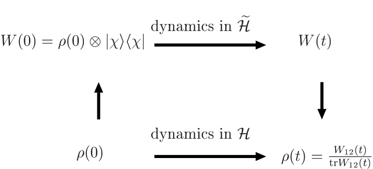
Figure 1: Illustration of the embedding theorem: The initial density matrix $\rho(0)$ evolves into $\rho(t)$ according to the given non-Markovian master equation (III.1). This evolution can be embedded in a Markovian dynamics on the extended state space $\widetilde{\mathcal{H}}={\mathcal{H}}\otimes{\mathbb{C}}^{3}$ in which the density matrix $W(0)$ evolves into $W(t)$ following the master equation (1).

Our aim is to show that by an appropriate choice of the Hamiltonian $H(t)$ and of the Lindblad operators $J_{i}(t)$ in Eq. (1) one can always achieve that the density matrix $\rho(t)$ on ${\mathcal{H}}$ is connected to the density matrix $W(t)$ on $\widetilde{\mathcal{H}}$ by means of the relation (${\mathrm{tr}}$ denotes the trace):

$$\rho(t)=\frac{W_{12}(t)}{{\mathrm{tr}}W_{12}(t)}.$$ (29)

Here, we have defined

$$W_{12}(t)=\langle 1|W(t)|2\rangle,$$ (30)

which is an operator acting on ${\mathcal{H}}$. We can regard this operator $W_{12}(t)$ as a matrix which is formed by the coherences (off-diagonal elements) of $W(t)$ between states from the subspace ${\mathcal{H}}_{1}$ and states from the subspace ${\mathcal{H}}_{2}$.

This is the embedding theorem. It states that the non-Markovian dynamics of $\rho(t)$ can be expressed through the time evolution of a certain set of coherences $W_{12}(t)$ of a density matrix $W(t)$ on the extended space which follows a Markovian dynamics (see Fig. 1).

To proof the embedding theorem we first demonstrate that the relation (29) can be achieved to hold at time $t=0$. If $\rho(0)$ is any initial density matrix on ${\mathcal{H}}$ we define a corresponding density matrix on $\widetilde{\mathcal{H}}$ by

$$W(0) \equiv \rho(0)\otimes\frac{1}{2}\big{[}|1\rangle\langle 1|+|2\rangle\langle 2|+|1\rangle\langle 2|+|2\rangle\langle 1|\big{]}$$ (31)

$$= \rho(0)\otimes|\chi\rangle\langle\chi|,$$

where

$$|\chi\rangle=\frac{1}{\sqrt{2}}\big{[}|1\rangle+|2\rangle\big{]}$$ (32)

is a state vector of the auxiliary system. We thus obtain $W(0)$ by combining the open system in the state $\rho(0)$ with the three state system in the pure state $|\chi\rangle\langle\chi|$. It is obvious that $W(0)$ given by Eq. (31) is a true density matrix on the triple Hilbert space $\widetilde{\mathcal{H}}$, i. e., we have $W(0)\geq 0$ and ${\mathrm{tr}}W(t)=1$. Moreover, Eq. (31) yields:

$$\frac{W_{12}(0)}{{\mathrm{tr}}W_{12}(0)}=\frac{\langle 1|W(0)|2\rangle}{{\mathrm{tr}}\langle 1|W(0)|2\rangle}=\frac{\frac{1}{2}\rho(0)}{\frac{1}{2}{\mathrm{tr}}\rho(0)}=\rho(0),$$ (33)

which is Eq. (29) at time $t=0$.

To show that the relation (29) is valid for all times $t\geq 0$ we have to demonstrate that the right-hand side of this relation satisfies the non-Markovian master equation (III.1), provided the Lindblad operators $J_{i}(t)$ in Eq. (1) are chosen appropriately. To simplify the presentation we first treat the case that the master equation (III.1) only involves a single operator $C(t)$ and $D(t)$. Thus we write, suppressing the time arguments,

$$\frac{d}{dt}\rho = -i[H_{S},\rho]+C\rho D^{\dagger}+D\rho C^{\dagger}$$ (34)

$$-\frac{1}{2}\left\{D^{\dagger}C+C^{\dagger}D,\rho\right\}.$$

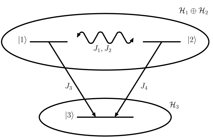
Figure 2: The extended state space ${\mathcal{H}}\otimes{\mathbb{C}}^{3}={\mathcal{H}}_{1}\oplus{\mathcal{H}}_{2}\oplus{\mathcal{H}}_{3}$ and the action of the operators $J_{i}$ defined in Eqs. (35)-(38).

We define four time dependent Lindblad operators for the master equation (1):

$$J_{1}(t) = C(t)\otimes|1\rangle\langle 1|+D(t)\otimes|2\rangle\langle 2|,$$ (35)

$$J_{2}(t) = D(t)\otimes|1\rangle\langle 1|+C(t)\otimes|2\rangle\langle 2|,$$ (36)

$$J_{3}(t) = \Omega(t)\otimes|3\rangle\langle 1|,$$ (37)

$$J_{4}(t) = \Omega(t)\otimes|3\rangle\langle 2|,$$ (38)

and the Hamiltonian:

$$H(t) = H_{S}(t)\otimes\big{[}|1\rangle\langle 1|+|2\rangle\langle 2|+|3\rangle\langle 3|\big{]}$$ (39)

$$\equiv H_{S}(t)\otimes I_{3},$$

where $I_{3}$ denotes the unit operator on the auxiliary space ${\mathbb{C}}^{3}$. In Eqs. (37) and (38) we have introduced a time dependent operator $\Omega(t)$ on ${\mathcal{H}}$ which will be defined below.

According to the definitions (35) and (36) the operators $J_{1}$ and $J_{2}$ leave invariant the subspace ${\mathcal{H}}_{1}\oplus{\mathcal{H}}_{2}$ which contains the states of the form $|\psi_{1}\rangle\otimes|1\rangle+|\psi_{2}\rangle\otimes|2\rangle$. The operators $J_{3}$ and $J_{4}$ defined in Eqs. (37) and (38) induce transitions $|1\rangle\rightarrow|3\rangle$ and $|2\rangle\rightarrow|3\rangle$ between the states of the auxiliary three state system. The extended state space and the action of the Lindblad operators are illustrated in Fig. 2.

We have from the above definitions (suppressing again the time arguments):

$$J_{1}^{\dagger}J_{1} = C^{\dagger}C\otimes|1\rangle\langle 1|+D^{\dagger}D\otimes|2\rangle\langle 2|,$$ (40)

$$J_{2}^{\dagger}J_{2} = D^{\dagger}D\otimes|1\rangle\langle 1|+C^{\dagger}C\otimes|2\rangle\langle 2|,$$ (41)

$$J_{3}^{\dagger}J_{3} = \Omega^{\dagger}\Omega\otimes|1\rangle\langle 1|,$$ (42)

$$J_{4}^{\dagger}J_{4} = \Omega^{\dagger}\Omega\otimes|2\rangle\langle 2|,$$ (43)

and:

$$\sum_{i=1}^{4}J_{i}^{\dagger}J_{i}=\left(\Omega^{\dagger}\Omega+C^{\dagger}C+D^{\dagger}D\right)\otimes\left(|1\rangle\langle 1|+|2\rangle\langle 2|\right).$$ (44)

With the Lindblad operators defined in Eqs. (35)-(38) and with the Hamiltonian given by Eq. (39) the master equation (1) leads to:

$$\frac{d}{dt}W_{12} = -i\langle 1|[H,W]|2\rangle+\sum_{i=1}^{4}\langle 1|J_{i}WJ_{i}^{\dagger}|2\rangle$$ (45)

$$-\frac{1}{2}\sum_{i=1}^{4}\langle 1|\big{\{}J_{i}^{\dagger}J_{i},W\big{\}}|2\rangle.$$

On using Eq. (44) we find

$$\sum_{i=1}^{4}\langle 1|\big{\{}J_{i}^{\dagger}J_{i},W\big{\}}|2\rangle=\left\{\Omega^{\dagger}\Omega+C^{\dagger}C+D^{\dagger}D,W_{12}\right\},$$ (46)

while Eqs. (35)-(39) yield

$$\langle 1|J_{1}WJ_{1}^{\dagger}|2\rangle = CW_{12}D^{\dagger},$$ (47)

$$\langle 1|J_{2}WJ_{2}^{\dagger}|2\rangle = DW_{12}C^{\dagger},$$ (48)

$$\langle 1|J_{3}WJ_{3}^{\dagger}|2\rangle = \langle 1|J_{4}WJ_{4}^{\dagger}|2\rangle=0,$$ (49)

$$\langle 1|[H,W]|2\rangle = [H_{S},W_{12}].$$ (50)

Employing the relations (46)-(50) in Eq. (45) we arrive at:

$$\frac{d}{dt}W_{12} = -i[H_{S},W_{12}]+CW_{12}D^{\dagger}+DW_{12}C^{\dagger}$$ (51)

$$-\frac{1}{2}\left\{\Omega^{\dagger}\Omega+C^{\dagger}C+D^{\dagger}D,W_{12}\right\}.$$

Here we see the reason for our choice of the extended state space and of the Lindblad operators $J_{i}$. The operators $J_{1}$ and $J_{2}$ have been chosen in such a way that $C$ acts from the left and $D^{\dagger}$ from the right on the coherences $W_{12}$, or vice versa [see Eqs. (47) and (48)]. On the other hand, since $J_{3}$ and $J_{4}$ induce transitions into the state $|3\rangle$ of the auxiliary system, the corresponding gain terms $J_{3}WJ^{\dagger}_{3}$ and $J_{4}WJ^{\dagger}_{4}$ of the master equation (1) do not contribute towards the equation of motion (51) for the coherences $W_{12}$ [see Eq. (49)]. The subspace ${\mathcal{H}}_{3}$ of the extended state space plays the role of a sink which will be used now to achieve that the loss terms of the master equation come out correctly.

We observe that Eq. (51) is already of a form which is similar to the desired master equation (34). These equations differ, however, with respect to the structure of the loss terms which are given by the terms containing the anti-commutator. To get an equation of motion of the desired form we now choose $\Omega$ to be a solution of the equation

$$\Omega^{\dagger}\Omega+C^{\dagger}C+D^{\dagger}D=aI+D^{\dagger}C+C^{\dagger}D,$$ (52)

which is equivalent to

$$\Omega^{\dagger}\Omega=aI-(C-D)^{\dagger}(C-D).$$ (53)

Here, $I$ denotes the unit operator on ${\mathcal{H}}$ and $a=a(t)$ is a time dependent non-negative number. Since $\Omega^{\dagger}\Omega$ is a positive operator a solution $\Omega$ of Eq. (53) exists under the condition that the right-hand side of Eq. (53) is also a positive operator. Thus, $a$ must be chosen in such a way that

$$a\geq||(C-D)|\psi\rangle||^{2}$$ (54)

for all normalized state vectors $|\psi\rangle$ in ${\mathcal{H}}$. We note that it is at this point that the assumption of bounded operators enters our construction. To make a definite choice we define $a$ to be the largest eigenvalue of the positive operator $(C-D)^{\dagger}(C-D)$. This definition ensures that the inequality (54) is satisfied and that a solution $\Omega$ of Eq. (53) exists.

The solution of Eq. (53) is, in general, not unique. If $\Omega$ is a solution, then also $U\Omega$, where $U$ is an arbitrary unitary operator. Changing $\Omega$ into $U\Omega$ does, however, not influence the equation of motion (51) since only the combination $\Omega^{\dagger}\Omega$ enters this equation. In the language of quantum measurement theory the transformation $\rho\mapsto\Omega\rho\Omega^{\dagger}$ is called a quantum operation KRAUS . It describes the change of a density matrix $\rho$ under a generalized measurement whose outcome occurs with probability ${\mathrm{tr}}(\Omega^{\dagger}\Omega\rho)$. We can thus say that the unitary operator $U$, expressing our freedom in the choice of $\Omega$, affects the change of the system state $\rho$, but not the probability of its occurrence.

Substituting Eq. (52) into Eq. (51) we get:

$$\frac{d}{dt}W_{12} = -i[H_{S},W_{12}]+CW_{12}D^{\dagger}+DW_{12}C^{\dagger}$$ (55)

$$-\frac{1}{2}\left\{D^{\dagger}C+C^{\dagger}D,W_{12}\right\}-aW_{12}.$$

We conclude from this equation that the trace of $W_{12}$ satisfies the equation

$$\frac{d}{dt}{\mathrm{tr}}W_{12}=-a{\mathrm{tr}}W_{12}.$$ (56)

Using this fact as well as Eq. (55) one immediately demonstrates that the expression on the right-hand side of Eq. (29) satisfies the desired master equation (34), which concludes the proof of the embedding theorem.

The general case of an arbitrary number of operators $C_{\alpha}(t)$ and $D_{\alpha}(t)$ in Eq. (III.1) can be treated in a similar way. To this end, one has to re-introduce the index $\alpha$ and to carry out a summation over $\alpha$ in the equations of motion. Thus, for each value of $\alpha$ we have a corresponding $\Omega_{\alpha}(t)$ and an $a_{\alpha}(t)$, as well as four $J_{i\alpha}(t)$, $i=1,2,3,4$.

Finally we note that according to Eq. (55) the operator $W_{21}\equiv\langle 2|W|1\rangle=W_{12}^{\dagger}$ satisfies the same differential equation as $W_{12}$. Since also $W_{21}(0)=W_{12}(0)$, we conclude that $W_{21}(t)=W_{12}(t)$ for all times. It follows that we can write for any operator $A$ on ${\mathcal{H}}$:

$${\mathrm{tr}}\left\{A\rho(t)\right\}=\frac{{\mathrm{tr}}\{(A\otimes\sigma_{x})W(t)\}}{{\mathrm{tr}}\{(I\otimes\sigma_{x})W(t)\}},$$ (57)

where

$$\sigma_{x}=|1\rangle\langle 2|+|2\rangle\langle 1|$$ (58)

is an operator on the auxiliary state space. This shows that the expectation value of all observables $A$ in the state $\rho(t)$ can be determined through measurements on the state $W(t)$ of the extended system.

III.3 Stochastic unraveling for non-Markovian processes

The embedding of the previous section enables us to construct a stochastic unraveling for the non-Markovian dynamics given by the master equation (III.1). Since the master equation governing $W(t)$ involves a time dependent Lindblad generator we can use the SSE developed in Sec. II.2 for this purpose.

The SSE (5) generates a stochastic process for the state vector $|\Phi(t)\rangle$ in the triple Hilbert space. Employing the representation (28) we write

$$|\Phi(t)\rangle=|\psi_{1}(t)\rangle\otimes|1\rangle+|\psi_{2}(t)\rangle\otimes|2\rangle+|\psi_{3}(t)\rangle\otimes|3\rangle.$$ (59)

As shown in Sec. II.2 the density matrix $W(t)$ on the extended state space is reproduced through the expectation value $W(t)=E[|\Phi(t)\rangle\langle\Phi(t)|]$, and the norm of the state vector is exactly conserved during the stochastic evolution:

$$\langle\Phi(t)|\Phi(t)\rangle$$ (60)

$$\equiv \langle\psi_{1}(t)|\psi_{1}(t)\rangle+\langle\psi_{2}(t)|\psi_{2}(t)\rangle+\langle\psi_{3}(t)|\psi_{3}(t)\rangle$$

$$= 1.$$

In accordance with Eq. (31) the initial state of the process is taken to be of the form:

$$|\Phi(0)\rangle=|\varphi\rangle\otimes|\chi\rangle=\frac{1}{\sqrt{2}}\left[|\varphi\rangle\otimes|1\rangle+|\varphi\rangle\otimes|2\rangle\right],$$ (61)

where $|\varphi\rangle$ is a normalized random state vector in ${\mathcal{H}}$, $\langle\varphi|\varphi\rangle=1$, and $|\chi\rangle$ is the fixed state vector of the auxiliary three state system defined in (32). We thus have $|\psi_{1}(0)\rangle=|\psi_{2}(0)\rangle=\frac{1}{\sqrt{2}}|\varphi\rangle$ and $|\psi_{3}(0)\rangle=0$. Hence, Eq. (29) at time $t=0$ gives

$$\rho(0)=E[|\varphi\rangle\langle\varphi|].$$ (62)

The embedding theorem now reveals that $\rho(t)$ is obtained from the stochastic evolution with the help of the relation [see Eq. (29)]:

$$\rho(t)=\frac{E(|\psi_{1}(t)\rangle\langle\psi_{2}(t)|)}{E(\langle\psi_{2}(t)|\psi_{1}(t)\rangle)}.$$ (63)

Thus we have constructed a stochastic unraveling for the non-Markovian dynamics. It is important to realize that our construction leads to an unraveling through a normalized stochastic state vector $|\Phi(t)\rangle$ and that the process allows a definite physical interpretation in terms of a continuous measurement, as has been discussed in Sec. II.2.

We remark that for the case $C=D$ the given master equation (34) is already in time dependent Lindblad form. Our construction then yields $a(t)=0$ [see inequality (54)] and $J_{1}=J_{2}$, as well as $J_{3}=J_{4}=0$. This means that the jump operators $J_{1}$ and $J_{2}$ are identical and that the decay channels $J_{3}$ and $J_{4}$ are closed. It follows that $|\psi_{3}(t)\rangle\equiv 0$ and that $|\psi_{1}\rangle$ evolves in exactly the same way as $|\psi_{2}\rangle$, that is, we have $|\psi_{1}(t)\rangle\equiv|\psi_{2}(t)\rangle$. Equation (63) thus becomes $\rho(t)=2E(|\psi_{1}(t)\rangle\langle\psi_{1}(t)|)$. Note that the factor $2$ is due to the normalization condition (60) which yields $\langle\psi_{1}|\psi_{1}\rangle=\langle\psi_{2}|\psi_{2}\rangle=1/2$. In the case $C=D$ our construction therefore reduces automatically to the standard unraveling of a master equation in Lindblad form.

IV Example

As an example we discuss a model for the non-Markovian decay of a two state system into the vacuum of a bosonic bath. The model serves to illustrate how to construct the embedding in a Markovian dynamics, and how to interpret physically the quantum trajectories generated by the resulting SSE.

IV.1 Construction of the process

The interaction picture master equation of the model is given by

$$\frac{d}{dt}\rho(t) = -i[H_{S}(t),\rho(t)]$$

$$+\gamma(t)\left(\sigma_{-}\rho(t)\sigma_{+}-\frac{1}{2}\left\{\sigma_{+}\sigma_{-},\rho(t)\right\}\right),$$

where

$$H_{S}(t)=\frac{1}{2}S(t)\sigma_{+}\sigma_{-}.$$ (65)

This is an exact master equation for the nonperturbative decay of a two state system with excited state $|e\rangle$ and ground state $|g\rangle$, which interacts with a bosonic bath TheWork . $\sigma_{+}=|e\rangle\langle g|$ and $\sigma_{-}=|g\rangle\langle e|$ are the usual raising and lowering operators of the two state system. These operators couple linearly to the bath through an interaction Hamiltonian of the form $\sigma_{-}Q^{\dagger}(t)+\sigma_{+}Q(t)$, where $Q(t)$ is a bath operator depending linearly on the annihilation operators of the bath modes.

The real functions $S(t)$ and $\gamma(t)$ are determined by the vacuum correlation function $\langle 0|Q(t)Q^{\dagger}(t_{1})|0\rangle$ of the bath. An example will be discussed below [see Eq. (91)]. The function $S(t)$ describes a time dependent renormalization of the system Hamiltonian induced by the coupling to the bath (Lamb shift). Under the condition $\gamma(t)\geq 0$ one can interpret the function $\gamma(t)$ as a time dependent decay rate of the excited state. But for certain spectral densities $\gamma(t)$ may become negative in certain time intervals such that the master equation (IV.1) is not in Lindblad form and the generator is not completely positive.

The master equation (IV.1) can however always be brought into the form of the non-Markovian master equation (34) by means of the definitions:

$$C(t) = \sqrt{\frac{|\gamma(t)|}{2}}\sigma_{-},$$ (66)

$$D(t) = \sqrt{\frac{|\gamma(t)|}{2}}{\mathrm{sign}}\gamma(t)\sigma_{-}.$$ (67)

To obtain the operator $\Omega(t)$ introduced in Eq. (53) we first have to determine the quantity $a=a(t)$ which is defined to be the largest eigenvalue of $(C-D)^{\dagger}(C-D)$. This operator is equal to $0$ for $\gamma(t)\geq 0$, and equal to $2|\gamma(t)|\sigma_{+}\sigma_{-}$ for $\gamma(t)<0$. Thus we find

$$(C-D)^{\dagger}(C-D)=a\sigma_{+}\sigma_{-}$$ (68)

and

$$a(t)=|\gamma(t)|-\gamma(t).$$ (69)

Hence, Eq. (53) takes the form

$$\Omega^{\dagger}\Omega = aI-(C-D)^{\dagger}(C-D)=a(I-\sigma_{+}\sigma_{-})$$ (70)

$$= a\sigma_{-}\sigma_{+},$$

which leads to an obvious solution:

$$\Omega(t)=\sqrt{a(t)}\sigma_{+}.$$ (71)

The Lindblad operators $J_{i}$ defined in Eqs. (35)-(38) are therefore given explicitly by:

$$J_{1} = \sqrt{\frac{|\gamma|}{2}}\sigma_{-}\otimes\big{[}|1\rangle\langle 1|+{\textrm{sign}}\gamma|2\rangle\langle 2|\big{]},$$ (72)

$$J_{2} = \sqrt{\frac{|\gamma|}{2}}\sigma_{-}\otimes\big{[}{\textrm{sign}}\gamma|1\rangle\langle 1|+|2\rangle\langle 2|\big{]},$$ (73)

$$J_{3} = \sqrt{a}\sigma_{+}\otimes|3\rangle\langle 1|,$$ (74)

$$J_{4} = \sqrt{a}\sigma_{+}\otimes|3\rangle\langle 2|.$$ (75)

IV.2 Physical interpretation

Considering times $t$ for which $\gamma(t)\geq 0$, we have $a=0$ [see Eqs. (69)] and, hence, $J_{3}=J_{4}=0$. This means that for $\gamma(t)\geq 0$ the decay channels described by $J_{3}$ and $J_{4}$ are closed: The process only involves the jumps of the state vector given by the operators $J_{1}$ and $J_{2}$. We infer from Eqs. (72) and (73) that $J_{1}$ and $J_{2}$ induce downward transitions $|e\rangle\rightarrow|g\rangle$ of the two state system (action of $\sigma_{-}$). These transitions result from the projection of the system’s state vector into the ground state $|g\rangle$ conditioned on the detection of a quantum in reservoir $R_{1}$ or $R_{2}$.

For $\gamma(t)<0$ the operators $J_{1}$ and $J_{2}$ again induce downward transitions of the two state system and, at the same time, introduce a relative phase factor of ${\textrm{sign}}\gamma=-1$ between the states $|1\rangle$ and $|2\rangle$ of the auxiliary three state system. Moreover, in the case $\gamma(t)<0$ the decay channels $J_{3}$ and $J_{4}$ are open: This enables the additional jumps of the state vector described by $J_{3}$ and $J_{4}$. Equations (74) and (75) show that $J_{3}$ and $J_{4}$ lead to upward transitions $|g\rangle\rightarrow|e\rangle$ of the two state system (action of $\sigma_{+}$) with simultaneous transitions between the auxiliary states of the form $|1\rangle\rightarrow|3\rangle$ or $|2\rangle\rightarrow|3\rangle$. A re-population of the excited state $|e\rangle$ is thus possible through jumps into the auxiliary state $|3\rangle$, corresponding to the detection of a quantum in reservoir $R_{3}$ or $R_{4}$.

A detailed analysis of the process can be given in terms of the statistics of the quantum jumps. To this end, we note that the waiting time distribution for the SSE (5) is given by

$$F(t_{1},t_{0})=1-\left|\left|T\exp\left[-i\int_{t_{0}}^{t_{1}}ds\hat{H}(s)\right]|\Phi(t_{0})\rangle\right|\right|^{2},$$ (76)

where $\hat{H}$ is defined by Eq. (8). $F(t_{1},t_{0})$ is the probability that a jump takes place in the time interval $(t_{0},t_{1})$, given that the previous jump occurred at time $t_{0}$ and yielded the state $|\Phi(t_{0})\rangle$. Note that this is a true cumulative probability distribution, i.e. $F(t_{1},t_{0})$ increases monotonically with $t_{1}$ and satisfies $F(t_{0},t_{0})=0$. For our model we have [see Eqs. (8), (39), (44) and (52)]:

$$\hat{H}(t) = H_{S}(t)\otimes I_{3}$$

$$-\frac{i}{2}\left(a(t)I+\gamma(t)\sigma_{+}\sigma_{-}\right)\otimes\left(|1\rangle\langle 1|+|2\rangle\langle 2|\right).$$

Let us analyze the process starting from the initial state

$$|\Phi(0)\rangle=|e\rangle\otimes|\chi\rangle,$$ (78)

and investigate the occupation probability $p_{g}(t)$ of the ground state. From the master equation it is clear that this quantity is given by the simple expression:

$$p_{g}(t)=1-\exp\left[-\int_{0}^{t}ds\gamma(s)\right].$$ (79)

If $\gamma(s)$ takes on positive and negative values, this is a non-monotonic function of time. Our aim is to illustrate how the stochastic dynamics reproduces this behavior and to explain the physical picture provided by the unraveling.

In the stochastic representation we have the formula [see Eq. (63)]:

$$p_{g}(t)=\frac{E[\langle g|\psi_{1}(t)\rangle\langle\psi_{2}(t)|g\rangle]}{E[\langle\psi_{2}(t)|\psi_{1}(t)\rangle]}.$$ (80)

We denote the moment of the first jump by $t_{1}$, the moment of the second jump by $t_{2}$. It follows from Eq. (76) that the waiting time distribution for the first jump is given by

$$F(t_{1},0)=1-\exp\left[-\int_{0}^{t_{1}}ds|\gamma(s)|\right],$$ (81)

and that the waiting time distribution for the second jump, given that the first jump took place at time $t_{1}$, becomes

$$F(t_{2},t_{1})=1-\exp\left[-\int_{t_{1}}^{t_{2}}dsa(s)\right].$$ (82)

We further denote the total number of jumps in the time interval $(0,t)$ by $N(t)$. Since the process starts from the state (78) the first jump is given by the application of $J_{1}$ or $J_{2}$ which project the state vector into the ground state. Therefore, prior to the first jump we have $2\langle g|\psi_{1}(t)\rangle\langle\psi_{2}(t)|g\rangle=0$, immediately afterwards we get $2\langle g|\psi_{1}(t)\rangle\langle\psi_{2}(t)|g\rangle={\mathrm{sign}}\gamma(t_{1})$. During the time intervals in which $\gamma(t)<0$ a second jump described by $J_{3}$ or $J_{4}$ is possible by which the state vector leaves the manifold ${\mathcal{H}}_{1}\oplus{\mathcal{H}}_{2}$ and lands in ${\mathcal{H}}_{3}$. Once the state vector is in ${\mathcal{H}}_{3}$, no further jumps are possible. Of course, we get again $2\langle g|\psi_{1}(t)\rangle\langle\psi_{2}(t)|g\rangle=0$ after the second jump. Summarizing we have three possible alternatives:

$$N(t)=0 \Rightarrow 2\langle g|\psi_{1}(t)\rangle\langle\psi_{2}(t)|g\rangle=0,$$ (83)

$$N(t)=1 \Rightarrow 2\langle g|\psi_{1}(t)\rangle\langle\psi_{2}(t)|g\rangle={\mathrm{sign}}\gamma(t_{1}),$$ (84)

$$N(t)=2 \Rightarrow 2\langle g|\psi_{1}(t)\rangle\langle\psi_{2}(t)|g\rangle=0.$$ (85)

From these relations we find the expectation value

$$E[2\langle g|\psi_{1}(t)\rangle\langle\psi_{2}(t)|g\rangle]$$

$$= \int_{0}^{t}dt_{1}\dot{F}(t_{1},0)[1-F(t,t_{1})]{\mathrm{sign}}\gamma(t_{1})$$

$$= \exp\left[-\int_{0}^{t}dt_{1}a(t_{1})\right]-\exp\left[-\int_{0}^{t}dt_{1}|\gamma(t_{1})|\right].$$

Here, the quantity $dt_{1}\dot{F}(t_{1},0)$ is the probability that the first jump occurs in $dt_{1}$, while $1-F(t,t_{1})$ is the probability that no further jumps take place within $(t_{1},t)$.

A similar analysis can be performed to obtain the expectation value of the quantity $2\langle\psi_{2}(t)|\psi_{1}(t)\rangle$. One finds:

$$N(t)=0 \Rightarrow 2\langle\psi_{2}(t)|\psi_{1}(t)\rangle=1,$$ (87)

$$N(t)=1 \Rightarrow 2\langle\psi_{2}(t)|\psi_{1}(t)\rangle={\mathrm{sign}}\gamma(t_{1}),$$ (88)

$$N(t)=2 \Rightarrow 2\langle\psi_{2}(t)|\psi_{1}(t)\rangle=0.$$ (89)

Thus we get:

$$E[2\langle\psi_{2}(t)|\psi_{1}(t)\rangle]$$ (90)

$$= 1-F(t,0)+\int_{0}^{t}dt_{1}\dot{F}(t_{1},0)[1-F(t,t_{1})]{\mathrm{sign}}\gamma(t_{1})$$

$$= \exp\left[-\int_{0}^{t}dt_{1}a(t_{1})\right].$$

The term $1-F(t,0)$ represents the no-jump probability, i. e., the contribution from the event $N(t)=0$. The result (90) could have been obtained also directly from Eq. (56). Using finally Eqs. (IV.2) and (90) in Eq. (80) we find, of course, the correct expression (79) for the excited state probability.

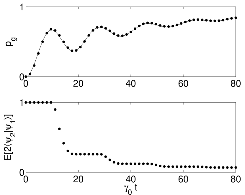
Figure 3: Simulation of the SSE (5) for the non-Markovian decay of a two-state system. Top: ground state probability $p_{g}$ obtained from a sample of $10^{5}$ quantum trajectories (dots), and analytical solution (continuous line). Bottom: expectation value $E[2\langle\psi_{2}|\psi_{1}\rangle]$. Parameters: $\gamma_{0}/\lambda=25$, $\Delta/\gamma_{0}=0.2$.

We illustrate the above analysis by means of an example. Figure 3 shows the results of a Monte Carlo simulation of the SSE (5) for the case of a Lorentzian spectral density which is detuned from the transition frequency of the two state system by an amount $\Delta$ (damped Jaynes-Cummings model). This leads to a bath correlation function of the form

$$\langle 0|Q(t)Q^{\dagger}(t_{1})|0\rangle=\frac{\gamma_{0}\lambda}{2}e^{i\Delta(t-t_{1})-\lambda|t-t_{1}|},$$ (91)

where $\gamma_{0}^{-1}$ is the Markovian relaxation time and $\lambda^{-1}$ is the correlation time of the bath. The simulation was carried out in a nonperturbative regime: While the Born-Markov approximation requires that $\gamma_{0}/\lambda\ll 1$, the simulation uses $\gamma_{0}/\lambda=25$. In this regime $\gamma(t)$ becomes negative for certain time intervals. These intervals can be seen in the figure as those intervals over which $p_{g}$ and $E[2\langle\psi_{2}|\psi_{1}\rangle]$ decrease monotonically with time. This is a signature for the fact that transitions $|1\rangle\rightarrow|3\rangle$ or $|2\rangle\rightarrow|3\rangle$ become possible through the channels $J_{3}$ or $J_{4}$. These channels are closed in the time intervals over which $E[2\langle\psi_{2}|\psi_{1}\rangle]$ stays constant.

The decrease of the ground state probability can be interpreted as due to virtual processes in which a quantum is emitted into the bath and re-absorbed at a later time. This is a clear non-Markovian feature of the dynamics. In the stochastic unraveling this decrease results from the contributions of those quantum trajectories which involve at least one jump and for which the first jump at time $t_{1}$ occurred during a phase in which $\gamma(t_{1})<0$. The first jump then yields a negative contribution to the expectation values of $2\langle g|\psi_{1}\rangle\langle\psi_{2}|g\rangle$ and of $2\langle\psi_{2}|\psi_{1}\rangle$ as a result of the relative phase factor ${\mathrm{sign}}\gamma(t_{1})=-1$ between the states $|1\rangle$ and $|2\rangle$ introduced by $J_{1}$ and $J_{2}$ [see Eqs. (84) and (88)]. Moreover, in a possible second jump the state vector leaves the manifold ${\mathcal{H}}_{1}\oplus{\mathcal{H}}_{2}$ to end up in a state proportional to $|e\rangle\otimes|3\rangle$, which gives $2\langle\psi_{2}|\psi_{1}\rangle=0$ [see Eq. (89)].

The decrease of $p_{g}$ is therefore due to quantum trajectories for which a second jump is possible which leads to a re-excitation $|g\rangle\rightarrow|e\rangle$. Thus we see that the virtual emission and re-absorption processes appear in the stochastic unraveling in the extended state space as certain real processes, namely as jumps with $J_{1}$ or $J_{2}$ involving a negative phase factor (detection of a quantum in reservoir $R_{1}$ or $R_{2}$), and as jumps into the auxiliary state $|3\rangle$ (detection of a quantum in reservoir $R_{3}$ or $R_{4}$). This shows how the quantum memory effect of virtual emission and re-absorption processes is encoded and completely stored in the continuous measurement record.

V Discussion and conclusions

In this paper we have developed a general method for the derivation of stochastic unravelings for non-Markovian quantum processes given by time-local master equations of the form (III.1). The key point of the construction is the fact that such master equations always allow a Markovian embedding in an extended state space with a rather simple structure, namely in the triple Hilbert space ${\mathcal{H}}\otimes{\mathbb{C}}^{3}$. Within this embedding the density matrix $\rho(t)$ of the original open system is expressed through a certain set of coherences of the full density matrix $W(t)$ on the extended state space.

The transition to the extended state space can be viewed physically as the addition of a further degree of freedom which is realized by a three level system. This enables one to represent the given non-Markovian dynamics by means of a suitable interaction with a Markovian environment consisting of the reservoirs $R_{i}$ introduced in Sec. II.2. Although the generator of the given non-Markovian master equation needs not be in Lindblad form, the corresponding dynamics in the extended state space is therefore governed by a time dependent Lindblad generator of the form of Eq. (1). The lifting to an appropriate extended state space thus allows the derivation of stochastic Schrödinger equations for non-Markovian dynamics through a consistent application of the standard theory of quantum measurement. The SSEs obtained in this way generate genuine quantum trajectories with the physical interpretation of continuous measurements.

The construction of Sec. III.2 provides a fairly general method for the Markovian embedding of a given non-Markovian dynamics: Apart from the existence of the master equation and from the boundedness of the operators $C_{\alpha}(t)$ and $D_{\alpha}(t)$, no assumption was made regarding the interaction Hamiltonian, the spectral density, the reservoir state, its temperature, etc. The Markovian embedding could therefore be useful in itself since it enables one to employ well established and developed concepts from the theory of completely positive maps and Lindblad generators in the study of non-Markovian master equations.

Formulating a non-Markovian unraveling we made use of piecewise deterministic jump processes. In an electromagnetic environment this corresponds, for example, to direct photodetection. It should be clear, however, that our derivation allows any unraveling in the extended state space. Alternatively one can use diffusion-type SSEs, which in a continuous measurement interpretation correspond to other detection schemes like homodyne or heterodyne photodetection WISEMAN1 ; WISEMAN2 .

Various stochastic unravelings for non-Markovian dynamics have been suggested in the literature, involving both jump processes IMAMOGLU ; JACK as well as SSEs with colored noise DGS1 ; DGS2 ; GAMBETTA1 ; GAMBETTA2 . The technique developed by Imamoglu IMAMOGLU is related to the method of pseudo modes GARRAWAY1 ; GARRAWAY2 . It employs an approximate Markovian embedding of a given non-Markovian dynamics. This embedding is based on the assumption that the reservoir can be represented by means of an effective set of fictitious damped harmonic oscillator modes. The Markovian embedding of the present paper is realized in an entirely different way by the introduction of the triple Hilbert space, and avoids the expansion into pseudo modes. It should also be noted that in the present method the density matrix $\rho(t)$ is not given by the partial trace of the density matrix $W(t)$ in the extended state space.

A further interesting method has been formulated by Diósi, Gisin and Strunz DGS1 ; DGS2 . These authors employ a nonlocal stochastic integro-differential equation for the state vector. As demonstrated by Gambetta and Wiseman GAMBETTA1 it seems, however, that the nonlocal SSE does not admit a continuous measurement interpretation within the framework of standard quantum measurement theory (see also GAMBETTA3 in this context). This means that measurements carried out at different times on the environment will influence the dynamics in a way which is incompatible with the stochastic process. The SSE does therefore not generate genuine quantum trajectories in the sense it does for Markovian dynamics.

A number of unravelings of non-Markovian dynamics has been proposed BKP ; STOCK which are based on the idea of propagating a pair $|\psi_{1}(t)\rangle$, $|\psi_{2}(t)\rangle$ of stochastic state vectors and of representing the reduced density matrix with the help of the expectation value $\rho(t)=E[|\psi_{1}(t)\rangle\langle\psi_{2}(t)|]$. It is even possible to design an exact stochastic unraveling PDP-EPJD ; PDP-PRA which neither requires the existence of a master equation nor a factorizing initial state. This method makes use of a pair of independently evolving product states in the state space of the total system. Related stochastic wave function methods have also been formulated for the description of bosonic and fermionic many-body systems CARUSO ; CHOMAZ , and for the simulation of quantum gases STEEL ; CORNEY by use of the positive P-representation DRUMMOND ; GILCHRIST . A measurement interpretation of these stochastic methods is however not available.

A pair $|\psi_{1}(t)\rangle$, $|\psi_{2}(t)\rangle$ of state vectors can be considered as an element of the double Hilbert space ${\mathcal{H}}\otimes{\mathbb{C}}^{2}\cong{\mathcal{H}}_{1}\oplus{\mathcal{H}}_{2}$ which is the tensor product of ${\mathcal{H}}$ and the state space of a two state system. In Ref. BKP a stochastic unraveling in the double Hilbert space has been constructed. Although this method has been demonstrated to provide a useful numerical tool, a continuous measurement interpretation seems again to be impossible. This is connected to the facts that not only the master equation in ${\mathcal{H}}$ but also the master equation in the double Hilbert space is generally not in Lindblad form and that the process does not preserve the norm of the state vector.

We mention finally some restrictions of the present theory. Similar to the formulation of the Lindblad theorem, we made use of the assumption of boundedness of the operators $C_{\alpha}(t)$ and $D_{\alpha}(t)$ in the non-Markovian master equation (III.1). This assumption excludes the immediate treatment of important cases, such as quantum Brownian motion which involves the unbounded operators for position and momentum of the particle. However, what is really needed in the proof is that the inequality (54) is satisfied. Provided the dynamics of the state vector is confined to an effective subspace of ${\mathcal{H}}$ on which the right-hand side of inequality (54) is bounded, we can still define a finite $a(t)$ and construct the embedding. A further restriction of the theory is that for certain models time-local master equation of the form (III.1) may not exist for very strong couplings. The latter can lead to singularities of the TCL generator and to a breakdown of the TCL expansion (an example is discussed in TheWork ). It is an important open problem whether a continuous measurement unraveling can be developed for such cases.

- (1) H. P. Breuer and F. Petruccione, The Theory of Open Quantum Systems (Oxford University Press, Oxford, 2002).
- (2) G. Lindblad, Commun. Math. Phys. 48, 119 (1976).
- (3) V. Gorini, A. Kossakowski, and E. C. G. Sudarshan, J. Math. Phys. 17, 821 (1976).
- (4) V. Gorini, A. Frigerio, M. Verri, A. Kossakowski, and E. C. G. Sudarshan, Rep. Math. Phys. 13, 149 (1978).
- (5) H. Carmichael, An Open Systems Approach to Quantum Optics, Vol. m18 of Lecture Notes in Physics (Springer-Verlag, Berlin, 1993).
- (6) J. Dalibard, Y. Castin, and K. Mølmer, Phys. Rev. Lett. 68, 580 (1992).
- (7) R. Dum, P. Zoller, and H. Ritsch, Phys. Rev. A 45, 4879 (1992).
- (8) M. B. Plenio and P. L. Knight, Rev. Mod. Phys. 70, 101 (1998).
- (9) N. Gisin and I. C. Percival, J. Phys. A: Math. Gen. 25, 5677 (1992).
- (10) H. M. Wiseman and G. J. Milburn, Phys. Rev. A 47, 642 (1993).
- (11) H. M. Wiseman and G. J. Milburn, Phys. Rev. A 47, 1652 (1993).
- (12) S. Nakajima, Progr. Theor. Phys. 20, 948 (1958).
- (13) R. Zwanzig, J. Chem. Phys. 33, 1338 (1960).
- (14) S. Chaturvedi and F. Shibata, Z. Phys. B 35, 297 (1979).
- (15) F. Shibata and T. Arimitsu, J. Phys. Soc. Jap. 49, 891 (1980).
- (16) A. Royer, Phys. Rev. A 6, 1741 (1972).
- (17) A. Royer, Phys. Lett. A 315, 335 (2003).
- (18) R. P. Feynman and F. L. Vernon, Ann. Phys. (N.Y.) 24, 118 (1963).
- (19) A. O. Caldeira and A. J. Leggett, Physica A 121, 587 (1983).
- (20) F. Haake and R. Reibold, Phys. Rev. A 32, 2462 (1985).
- (21) B. L. Hu, J. P. Paz and Y. Zhang, Phys. Rev. D 45, 2843 (1992).
- (22) R. Karrlein and H. Grabert, Phys. Rev. E 55, 153 (1997).
- (23) E. B. Davies and H. Spohn, J. Stat. Phys. 19, 511 (1978).
- (24) R. Alicki, J. Phys. A: Math. Gen. 12, L103 (1979).
- (25) Y. Castin and K. Mølmer, Phys. Rev. Lett. 74, 3772 (1995).
- (26) V. B. Braginsky and F. Ya. Khalili, Quantum Measurement (Cambridge University Press, Cambridge, 1992).
- (27) T.-M. Chang and J. L. Skinner, Physica A 193, 483 (1993).
- (28) L. D. Blanga and M. A. Despósito, Physica A 227, 248 (1996).
- (29) H. P. Breuer, B. Kappler, and F. Petruccione, Ann. Phys. (N.Y.) 291, 36 (2001).
- (30) H. P. Breuer, Eur. Phys. J. D (2004), in press (quant-ph/0309114).
- (31) H. P. Breuer, D. Burgarth, and F. Petruccione, quant-ph/0401051.
- (32) H. P. Breuer, D. Faller, B. Kappler, and F. Petruccione, Europhys. Lett. 54, 14 (2001).
- (33) H. P. Breuer and F. Petruccione, Phys. Rev. A 63, 032102 (2001).
- (34) K. Kraus, States, Effects, and Operations, Vol. 190 of Lecture Notes in Physics (Springer-Verlag, Berlin, 1983).
- (35) A. Imamoglu, Phys. Rev. A 50, 3650 (1994).
- (36) M. W. Jack and M. J. Collett, Phys. Rev. A 61, 062106 (2000).
- (37) L. Diósi, N. Gisin, and W. T. Strunz, Phys. Rev. A 58, 1699 (1998).
- (38) W. T. Strunz, L. Diósi, and N. Gisin, Phys. Rev. Lett. 82, 1801 (1999).
- (39) J. Gambetta and H. M. Wiseman, Phys. Rev. A 66, 012108 (2002).
- (40) J. Gambetta and H. M. Wiseman, Phys. Rev. A 66, 052105 (2002).
- (41) B. M. Garraway, Phys. Rev. A 55, 2290 (1997).
- (42) B. M. Garraway, Phys. Rev. A 55, 4636 (1997).
- (43) J. Gambetta and H. M. Wiseman, Phys. Rev. A 68, 062104 (2003).
- (44) H. P. Breuer, B. Kappler, and F. Petruccione, Phys. Rev. A 59, 1633 (1999).
- (45) J. T. Stockburger and H. Grabert, Phys. Rev. Lett. 88, 170407 (2002).
- (46) H. P. Breuer, Phys. Rev. A 69, 022115 (2004).
- (47) I. Carusotto, Y. Castin, and J. Dalibard, Phys. Rev. A 63, 023606 (2001).
- (48) O. Juillet and Ph. Chomaz, Phys. Rev. Lett. 88, 142503 (2002).
- (49) M. J. Steel, M. K. Olsen, L. I. Plimak, P. D. Drummond, S. M. Tan, M. J. Collett, D. F. Walls, and R. Graham, Phys. Rev. A 58, 4824 (1998).
- (50) P. D. Drummond and J. F. Corney, Phys. Rev. A 60, R2661 (1999).
- (51) P. D. Drummond and C. W. Gardiner, J. Phys. A: Math. Gen. 13, 2353 (1980).
- (52) A. Gilchrist, C. W. Gardiner, and P. D. Drummond, Phys. Rev. A 55, 3014 (1997).