Two-photon nonlinearity in general cavity QED systems

Abstract

We have investigated the two-photon nonlinearity at general cavity QED systems, which covers both weak and strong coupling regimes and includes radiative loss from the atom. The one- and two-photon propagators are obtained in analytic forms. By surveying both coupling regimes, we have revealed the conditions on the photonic wavepacket for yielding large nonlinearity depending on the cavity Q-value. We have also discussed the effect of radiative loss on the nonlinearity.

I Introduction

The nonlinear optical response appears strongly when intense light fields are irradiated onto the material with large nonlinearities. By using an optical cavity, we can magnify the intensity of the input field inside the cavity, if the input field is resonant to the cavity mode QOpt . Thus, we can enhance the nonlinear optical response by putting the nonlinear material inside the cavity. This is realized experimentally by using two-level atoms as the nonlinear material Kimble1 ; Kimble2 . This idea opened the possibility of obtaining large nonlinearity even by weak input fields. In particular, the nonlinearity appearing in the two-photon state is attracting much attention due to its possible application to quantum information devices Nie and to recent progresses in the photon-pair manipulation technique Take ; Eda .

In order to discuss the dynamics of two-photon state theoretically, quantum-mechanical treatment of the photon field is indispensable, because the nonlinearity appears in the wavefunction of the photon, not in the amplitude cm:number . Such an analysis was pioneered in a case where the nonlinear material is a one-dimensional atom, which is obtained as the lossless and weak-coupling limit of the atom-cavity system KojHof . However, considering that the photon field is more magnified for better (higher Q-value) cavities, the strong-coupling cases also seem promising in yielding large nonlinearity Ajiki . The optimum cavity conditions for the two-photon nonlinearity have not been sufficiently discussed, which should be studied with the method applicable to any coupling regime. In this study, we derive the analytic expression of the two-photon propagator in general atom-cavity system, where both weak and strong coupling regimes are covered and the loss from the cavity due to radiative decay into non-cavity modes is taken into account. Using this propagator, we discuss the two-photon nonlinearity, and clarify the optimum condition on the photonic wavepacket for achieving large nonlinearity depending on the cavity conditions.

The composition of this paper is as follows. In Sec. II, the theoretical model of the atom-cavity system is introduced, and the meanings of the parameters are described. In Sec. III, we define the input and output states of photons. In Sec. IV, the measure of the nonlinearity appearing in the output state is defined. In Sec. V, we show the form of the input wavefunction and a scaling law for this atom-cavity system. In Sec. VI, we numerically evaluate the nonlinearity for the lossless case, and clarify the optimum condition for inducing large nonlinearity. In Sec. VII, the effect of the loss is discussed. The analytic expressions for the one- and two-photon propagators are shown in Appendix.

II System

As the nonlinear optical system, we here investigate a single two-level system (hereafter called an “atom”) embedded in a one-sided cavity CQED . The system is schematically illustrated in Fig. 1. The atom is coupled, besides the cavity mode, to the photon field in the lateral direction. The cavity mode is coupled through the right mirror of the cavity to the external photon field, which is labeled one-dimensionally by $r$. Although the external field actually extends only in the $r>0$ region and the incoming and outgoing photons are flying in the opposite direction, we treat the incoming photons to propagate in the $r<0$ region in the positive direction Hof2 .

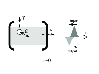
Figure 1: Schematic view of the atom-cavity system. The right mirror of the cavity is weakly transmissive, through which the cavity mode is coupled to the external photon field. $g$, $\gamma$, $\kappa$ represents the atom-cavity coupling, the radiative decay rate of the atom into lateral photon modes, and the decay rate of the cavity mode, respectively.

The Hamiltonian of the system is given, putting $\hbar=c=1$, by

$${\cal H} = \omega_{a}\sigma_{+}\sigma_{-}+\int d\mu\ \mu d_{\mu}^{\dagger}d_{\mu}+\int d\mu\ (\gamma_{\mu}\sigma_{+}d_{\mu}+h.c.)$$ (1)

$$+ \omega_{c}c^{\dagger}c+\int dk\ kb_{k}^{\dagger}b_{k}+\int dk\ (\kappa_{k}c^{\dagger}b_{k}+h.c.)$$

$$+ g(\sigma_{+}c+c^{\dagger}\sigma_{-}),$$

where $\sigma_{-}$, $c$, $b_{k}$, and $d_{\mu}$ are the annihilation operators for the atom, cavity mode, external photon mode, and lateral photon mode, respectively. $\omega_{a}$ and $\omega_{c}$ represent the frequencies of the atomic transition and the cavity mode, and $g$ represents the atom-cavity coupling. Regarding $\gamma_{\mu}$ and $\kappa_{k}$, we use the flat-band assumption, i.e., $\gamma_{\mu}=(\gamma/2\pi)^{1/2}$ and $\kappa_{k}=(\kappa/2\pi)^{1/2}$, by which the damping rates of the atom and the cavity mode are given by $\gamma$ and $\kappa$.

The complex frequencies of the atom and cavity are defined by

$$\tilde{\omega}_{a}=\omega_{a}-i\gamma/2,$$ (2)

$$\tilde{\omega}_{c}=\omega_{c}-i\kappa/2.$$ (3)

Using these frequencies, the complex eigenfrequencies $\tilde{\omega}_{1,2}$ of the atom-cavity system are given by

$$(\omega-\tilde{\omega}_{1})(\omega-\tilde{\omega}_{2})=(\omega-\tilde{\omega}_{a})(\omega-\tilde{\omega}_{c})-g^{2}.$$ (4)

We remark here that $\gamma$ is related to the dissipation of this atom-cavity system. When $\gamma=0$, the inputted photons are always reflected back into the output port, i.e., the atom-cavity system is lossless. Contrarily, when $\gamma\neq 0$, some of the inputted photons are lost as the spontaneous emission into the lateral direction, i.e., the atom-cavity system is lossy. We also remark that, in the limit of $\gamma\to 0$ and $(g,\kappa)\to\infty$ keeping $\Gamma=4g^{2}/\kappa$ constant, this atom-cavity system is reduced to the one-dimensional atom, where the atom is directly coupled to the external field at $r=0$ with the coupling constant $\Gamma$ Kimble1 ; KojHof .

The real-space operator of the external field, $b_{r}$, is given by the Fourier transform of $b_{k}$;

$$b_{r}=(2\pi)^{-1/2}\int dke^{{\rm i}kr}b_{k}.$$ (5)

We note again that the negative (positive) $r$ represents the incoming (outgoing) fields.

III input and output states

Our main concern in this study is how the initial one- or two-photon wavepackets are transformed after the interaction with the atom-cavity system. In the initial state, the atom-cavity system is in the ground state and one or two photons exist in the input port, i.e.,

$$|\Psi^{(1)}_{\rm in}\rangle = \int dr\psi_{\rm in}(r)b_{r}^{\dagger}|0\rangle,$$ (6)

$$|\Psi^{(2)}_{\rm in}\rangle = 2^{-1/2}\int dr_{1}dr_{2}\psi_{\rm in}(r_{1},r_{2})b_{r_{1}}^{\dagger}b_{r_{2}}^{\dagger}|0\rangle.$$ (7)

The one-photon wavefunction $\psi_{\rm in}(r)$ is normalized as $\int dr|\psi_{\rm in}(r)|^{2}=1$, and $\psi_{\rm in}(r)=0$ in $r>0$. Similarly, $\psi_{\rm in}(r_{1},r_{2})$ satisfies $\int dr_{1}dr_{2}|\psi_{\rm in}(r_{1},r_{2})|^{2}=1$ and $\psi_{\rm in}(r_{1},r_{2})=0$ in $r_{1},r_{2}>0$, and has the symmetry $\psi_{\rm in}(r_{2},r_{1})=\psi_{\rm in}(r_{1},r_{2})$.

Sufficiently after the photons have interacted with this atom-cavity system, the excitations in the atom and the cavity mode completely escape to the external modes ($b_{k}$) or to the lateral modes ($d_{\mu}$). Then, the states of the system are written as

$$|\Psi^{(1)}_{\rm out}\rangle = \int dr\psi_{\rm out}(r)b_{r}^{\dagger}|0\rangle+\cdots,$$ (8)

$$|\Psi^{(2)}_{\rm out}\rangle = 2^{-1/2}\int dr_{1}dr_{2}\psi_{\rm out}(r_{1},r_{2})b_{r_{1}}^{\dagger}b_{r_{2}}^{\dagger}|0\rangle+\cdots,$$ (9)

where the dots imply the terms containing the lateral mode excitations. While the number of the photons are kept in the output wavepacket ($\int dr|\psi_{\rm out}(r)|^{2}=1$ and $\int dr_{1}dr_{2}|\psi_{\rm out}(r_{1},r_{2})|^{2}=1$) in case of $\gamma=0$, the output state is attenuated in general cases of $\gamma\neq 0$.

The input and the output wavefunctions are related by the propagator $G$ as follows;

$$\psi_{\rm out}(r) = \int dr^{\prime}G(r;r^{\prime})\psi_{\rm in}(r^{\prime}),$$ (10)

$$\psi_{\rm out}(r_{1},r_{2}) = \int dr^{\prime}_{1}dr^{\prime}_{2}G(r_{1},r_{2};r^{\prime}_{1},r^{\prime}_{2})\psi_{\rm in}(r^{\prime}_{1},r^{\prime}_{2}).$$ (11)

The one- and two-photon propagators are analytically obtainable for this atom-cavity system, which are shown in the appendix. The two-photon propagator has the symmetry of $G(r_{2},r_{1};r^{\prime}_{2},r^{\prime}_{1})=G(r_{1},r_{2};r^{\prime}_{1},r^{\prime}_{2})$, which guarantees the symmetry in the output wavefunction, $\psi_{\rm out}(r_{2},r_{1})=\psi_{\rm out}(r_{1},r_{2})$.

IV measure of nonlinearity

When two photons are inputted into this atom-cavity system, the input wavefunction $\psi_{\rm in}(r_{1},r_{2})$ is finally transformed to the output wavefunction $\psi_{\rm out}(r_{1},r_{2})$. In order to quantify the nonlinear effect in this process, we compare $\psi_{\rm out}(r_{1},r_{2})$ with the linear output wavefunction $\psi_{\rm out}^{\rm L}(r_{1},r_{2})$, which is defined by

$$\psi_{\rm out}^{\rm L}(r_{1},r_{2})=\int dr^{\prime}_{1}dr^{\prime}_{2}G(r_{1};r^{\prime}_{1})G(r_{2};r^{\prime}_{2})\psi_{\rm in}(r^{\prime}_{1},r^{\prime}_{2}),$$ (12)

where $G(r;r^{\prime})$ is the one-photon propagator. This linear output is obtained when the atom in the cavity is replaced by a harmonic oscillator with the same transition frequency, i.e., when the nonlinearity of the system is completely removed.

We here define the following quantity $\beta$ by

$$\beta=\frac{\int dr_{1}dr_{2}(\psi_{\rm out}^{\rm L})^{\ast}\psi_{\rm out}}{\sqrt{\int dr_{1}dr_{2}|\psi_{\rm out}|^{2}}\sqrt{\int dr_{1}dr_{2}|\psi_{\rm out}^{\rm L}|^{2}}}.$$ (13)

$\beta$ always lies in the unit circle ($|\beta|\leq 1$) due to the Schwartz’s inequality, and $\beta=1$ holds when the response of the system is completely linear ($\psi_{\rm out}=\psi_{\rm out}^{\rm L}$). Thus, the nonlinear effect is reflected in the deviation of $\beta$ from the unity, and $|\beta-1|$ may be regarded as a measure of the nonlinear effect. We also note that, when the atom-cavity system is lossless ($\gamma=0$), the norms of $\psi_{\rm out}$ and $\psi_{\rm out}^{\rm L}$ in the denominator are always unity, and $\beta$ is simply reduced to the overlap integral between $\psi_{\rm out}$ and $\psi_{\rm out}^{\rm L}$.

V input wavefunctions and scaling law

Now we embody the above formalism for specific forms of the input states, and clarify the conditions to obtain large nonlinearity between two photons. In this study, we focus on the case where the two input photons have the same wavefunction of the Gaussian form, i.e.,

$$\psi_{\rm in}(r_{1},r_{2}) = \psi_{\rm in}(r_{1}-a)\ \psi_{\rm in}(r_{2}-a),$$ (14)

$$\psi_{\rm in}(r) = (2/\pi d^{2})^{1/4}\exp(-r^{2}/d^{2}+iqr).$$ (15)

The input wavefunction is characterized by two parameters, $q$ (the central frequency) and $d$ (the coherent length of the photon). $a(<0)$ in Eq. (14) represents the initial position of the photons, which is an irrelevant parameter.

The atom-cavity system is characterized by $g$ (the coupling between the atom and the cavity mode), $\omega_{a}-\omega_{c}$ (the frequency mismatch between the atom and the cavity mode), $\gamma$ (the damping rate of the atom into the lateral modes), and $\kappa$ (the damping rate of the cavity mode), Adding the input-photon parameters $q$ and $d$, the whole system is specified by the following set of parameters, $(g,\omega_{a}-\omega_{c},\gamma,\kappa,q,d)$. However, the number of the parameters may be decreased with the help of the scaling law that the system with the parameters $(\alpha g,\alpha(\omega_{a}-\omega_{c}),\alpha\gamma,\alpha\kappa,\alpha q,d/\alpha)$ is equivalent to the one with $(g,\omega_{a}-\omega_{c},\gamma,\kappa,q,d)$, where $\alpha$ is a positive constant. Using this law, the system is specified by the following set of dimensionless parameters, $((\omega_{a}-\omega_{c})/g,\gamma/g,\kappa/g,q/g,gd)$. $\omega_{a}-\omega_{c}$ is fixed at zero in the following numerical examples, and $\omega_{a}$ (=$\omega_{c}$) is chosen as the origin of frequency.

VI numerical results for lossless cases

In this section, we show the numerical results for $\gamma=0$ cases, where the atom-cavity system is lossless and the number of photons is preserved in the output wavepacket. The atom-cavity system is then characterized only by the ratio $\kappa/g$, as has been discussed in Sec. V. Eq. (4) indicates that the Rabi splitting of the eigenfrequency of the atom-cavity system takes place when $\kappa/g<4$. Thus, in our definition of the parameters, the strong (weak) coupling regime is specified by $\kappa/g\lesssim 4$ ($\kappa/g\gtrsim 4$).

VI.1 Weak coupling regime

First, we discuss the weak coupling regime. In Fig. 2, the nonlinearity $|\beta-1|$ is plotted for the cases of resonant input ($q=0$) as a function of $\kappa/g$ and $g^{2}d/\kappa$. It has been confirmed that the nonlinearity appears most strongly at $q=0$ in the weak coupling regime and the nonlinearity gets weaker as $|q|$ is increased.

Fig. 2 indicates that, roughly speaking, the nonlinearity $|\beta-1|$ is dependent solely on $g^{2}d/\kappa$ in the weak coupling regime ($\kappa/g\gtrsim 4$). This is because, in the weak coupling regime, the atom-cavity system may be regarded as a “one-dimensional atom”, where the atom is coupled directly to a one-dimensional photon field with a coupling constant $4g^{2}/\kappa$. It is observed that the nonlinearity is maximized when $g^{2}d/\kappa\sim 0.5$. For example, for $g=$120MHz and $\kappa$=900MHz Kimble2 , the optimum pulse length $d$ is about 9m. The qualitative explanation for this optimum condition will be given in Sec. VI.3.

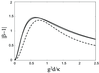
Figure 2: Dependence of $|\beta-1|$ on $g^{2}d/\kappa$, where $\kappa/g=10$ (solid line), $\kappa/g=5$ (dotted line), and $\kappa/g=2$ (broken line). The frequency of the photons are resonant to the cavity mode ($q=0$).

VI.2 Strong coupling regime

Next, we discuss the strong coupling regime. In Fig. 3, the nonlinearity $|\beta-1|$ is plotted for the fixed $\kappa/g$(=0.5) as a function of $\kappa d$ and $q/g$. Contrarily to the weak coupling case, the nonlinearity is weak for the resonant input ($q=0$). This is because the $q=0$ photons are no more resonant to the cavity mode due to the Rabi splitting. Instead, the nonlinearity appears strongly when the input photons are tuned to the Rabi-splitted resonant frequency, $q\sim\pm g$. The maximum value of $|\beta-1|$ is about 1.5, which is almost the same as the weak coupling case. The nonlinearity is optimized for $\kappa d\sim 4$, the reason of which will be discussed in Sec. VI.3.

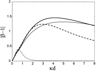
Figure 3: Dependence of $|\beta-1|$ on $\kappa d$, where $\kappa/g$ is fixed at 0.5 (strong coupling regime). $q/g=0.8$ (broken line), $q/g=0.9$ (solid line), $q/g=1$ (dotted line), and $q/g=0$ (thin broken line).

VI.3 Optimum pulse for inducing large nonlinearity

In the preceding subsections, we have clarified the optimum frequency $q$ and the length $d$ of the photon pulse for inducing large nonlinearity, in both weak and strong coupling regimes. Here we explain these optimum conditions from a unified viewpoint. To this end, we focus on the following wavefunction $\varphi(r)$, which is defined by

$$e^{i{\cal H}t}\sigma_{+}|0\rangle=\int dr\varphi(r)b_{r}^{\dagger}|0\rangle$$ (16)

for large $t(>0)$. The meaning of $\varphi(r)$ becomes clear by multiplying $e^{-i{\cal H}t}$ from the left; if a single photon pulse $\varphi(r)$ is prepared as an input at time $t_{0}$, the photon will completely be absorbed by the atom at time $t_{0}+t$. Therefore, it is expected that, when the input pulse $\psi_{\rm in}(r)$ resembles $\varphi(r)$ in shape, the two input photons try to occupy the atom simultaneously and the nonlinearity appears strongly.

$\varphi(r)$ has the following form;

$$\varphi(r)=\left\{\begin{array}[]{lr}\frac{ig\kappa^{1/2}}{\tilde{\omega}_{1}^{\ast}-\tilde{\omega}_{2}^{\ast}}(e^{i\tilde{\omega}_{1}^{\ast}(r+t)}-e^{i\tilde{\omega}_{2}^{\ast}(r+t)})&(-t<r<0)\\ 0&({\rm otherwise})\end{array}\right.,$$ (17)

where $\tilde{\omega}_{1}$ and $\tilde{\omega}_{2}$ are the complex eigenfrequencies of the atom-cavity system, defined in Eq. (4). In the weak coupling regime, $\tilde{\omega}_{1,2}$ are approximately given by $-i\kappa/2$ and $-2ig^{2}/\kappa$. Noticing that $g^{2}/\kappa\gg\kappa$ in this regime, the optimum frequency $q$ and pulse length $d$ are given by $q\sim 0$ and $d\sim\kappa/2g^{2}$, which explains the numerical results in Sec. VI.1. On the other hand, in the strong coupling regime, $\tilde{\omega}_{1,2}$ are approximately given by $-i\kappa/4\pm g$. Therefore, the optimum $q$ and $d$ are roughly estimated at $q\sim\pm g$ and $d\sim 4/\kappa$, which are in agreement with the numerical results in Sec. VI.2.

VII numerical results for lossy cases

In the preceding section, the results for the lossless cases ($\gamma=0$) are presented. Here, we discuss the lossy cases ($\gamma\neq 0$), fixing the parameters $\kappa/g=5$ (weak coupling regime) and $q=0$ for example.

The apparent result of the presence of the loss is attenuation of the photon pulses. In Fig. 4, we have plotted the norm of the two-photon output wavefunction $\psi_{\rm out}(r_{1},r_{2})$, i.e., the probability to find two photons in the output. The norm of the linear output wavefunction $\psi_{\rm out}^{\rm L}(r_{1},r_{2})$ is also plotted in the same figure. As expected, the photon pulse is attenuated more significantly when the loss parameter $\gamma$ is larger, for both $\psi_{\rm out}$ and $\psi_{\rm out}^{\rm L}$ (compare solid and broken lines). It is also observed that $\psi_{\rm out}^{\rm L}$ is more attenuated than $\psi_{\rm out}$. This is understood by the facts that, in the linear case, the photons are more likely to be absorbed by the atom due to the absence of the saturation effect, and that the loss of photons may take place only while the photons are occupying the atom, as schematically shown in Fig. 1.

Fig. 5 plots the nonlinear parameter $|\beta-1|$ defined in Eq. (13), when the system has finite loss $\gamma$. It is observed that $|\beta-1|$ is slightly decreased (increased) for $g^{2}d/\kappa\lesssim 0.5$ ($g^{2}d/\kappa\gtrsim 0.5$) region but, overall, that no qualitative changes are introduced by the presence of the loss. Thus, although the probability to find two photons in the output is largely decreased as shown in Fig. 4, the nonlinear characteristics of the output state are almost unchanged from the lossless case if the output pulse contains two photons.

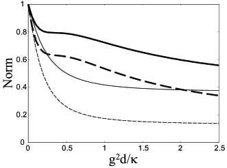
Figure 4: Norms of $\psi_{\rm out}(r_{1},r_{2})$ (bold lines) and $\psi_{\rm out}^{\rm L}(r_{1},r_{2})$ (thin lines), for lossy cases of $\gamma/g=0.1$ (solid lines) and $\gamma/g=0.1$ (broken lines). The atom-cavity system is in the weak coupling regime ($\kappa/g=5$) and the resonant photons ($q=0$) are used.

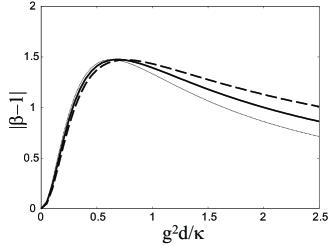
Figure 5: Effect of the loss on the nonlinearity $|\beta-1|$; $\gamma/g=0$ (thin dotted line), $\gamma/g=0.1$ (solid line), and $\gamma/g=0.2$ (broken line). Other parameters are $\kappa/g=5$ and $q=0$.

VIII summary

We have theoretically investigated a situation where two photons are simultaneously inputted into a nonlinear optical system, and examined the nonlinear effect in the output wavepacket. As a model nonlinear optical system, we employed a two-level system (atom) embedded in a cavity, which is illustrated in Fig. 1. The one- and two-photon propagators are obtained in analytic forms, which are presented in Appendix. The overlap integral of the linear and nonlinear two-photon output wavepackets, Eq. (13), is used to measure the nonlinear effect. This quantity is numerically evaluated both in the weak coupling regime (Fig. 2) and in the strong coupling regime (Fig. 3), and the conditions for inducing large nonlinearity is revealed. These conditions are explained by the optimum pulse shape, Eq. (17). This finding suggests that the pulse shape control is more essential in optimizing the two-photon nonlinearity rather than the Q-value control of the cavity system. We also considered the $\gamma\neq 0$ cases, where the atom-cavity system is lossy. As shown in Fig. 4, the probability to find two photons in the output is largely decreased by the effect of the loss, but the nonlinear characteristics of the output two-photon output state are almost unchanged from the lossless case.

Appendix A propagator

In this section, we present the analytic forms of the one- and two-photon propagators $G(r;r^{\prime})$ and $G(r_{1},r_{2};r^{\prime}_{1},r^{\prime}_{2})$. Using the completeness relation in the one-photon space, $\hat{1}=\int drb_{r}^{\dagger}|0\rangle\langle 0|b_{r}$, the one-photon propagator is given by

$$G(r;r^{\prime})=\langle 0|b_{r}e^{-{\rm i}{\cal H}t}b_{r^{\prime}}^{\dagger}|0\rangle,$$ (18)

where $r>0>r^{\prime}$, and $t$ is the time difference between the output and the input. This propagators are derivable by standard application of the Green function method Mahan . Throughout this section, we use the coordinate system moving at the light speed; transformation to the static coordinate system is done by replacing $r$ (coordinates without primes) by $r-t$, or $r^{\prime}$ (coordinates with primes) by $r^{\prime}+t$. In this coordinate system, the one-photon propagator is identified as

$$G(r,r^{\prime}) = G(r-r^{\prime})=G_{0}(r-r^{\prime})+G_{2}(r-r^{\prime}),$$ (19)

$$G_{0}(r-r^{\prime}) = \delta(r-r^{\prime})-\kappa\theta(r^{\prime}-r)e^{{\rm i}\tilde{\omega}_{c}(r-r^{\prime})},$$ (20)

$$G_{2}(r-r^{\prime}) = \kappa\theta(r^{\prime}-r)\left(e^{{\rm i}\tilde{\omega}_{c}(r-r^{\prime})}-\frac{\tilde{\omega}_{2}-\tilde{\omega}_{c}}{\tilde{\omega}_{2}-\tilde{\omega}_{1}}e^{{\rm i}\tilde{\omega}_{1}(r-r^{\prime})}-\frac{\tilde{\omega}_{1}-\tilde{\omega}_{c}}{\tilde{\omega}_{1}-\tilde{\omega}_{2}}e^{{\rm i}\tilde{\omega}_{2}(r-r^{\prime})}\right),$$ (21)

where $\tilde{\omega}_{a}$ (complex frequency of the atom), $\tilde{\omega}_{c}$ (complex frequency of the cavity), and $\tilde{\omega}_{1,2}$ (complex eigenfrequencies of the atom-cavity system) are defined in Eqs. (2), (3), and (4).

Next, we proceed to the two-photon case. Using the completeness relation in the two-photon space, $\hat{1}=2^{-1}\int dr_{1}dr_{2}b_{r_{1}}^{\dagger}b_{r_{2}}^{\dagger}|0\rangle\langle 0|b_{r_{1}}b_{r_{2}}$, the two-photon propagator is identified as $2^{-1}\langle 0|b_{r_{1}}b_{r_{2}}e^{-{\rm i}{\cal H}t}b_{r^{\prime}_{1}}^{\dagger}b_{r^{\prime}_{2}}^{\dagger}|0\rangle$. This quantity is composed of two kinds of terms; in the first (second) kind, the photons initially located at $r^{\prime}_{1}$ and $r^{\prime}_{2}$ are scattered to $r_{1}$ and $r_{2}$ ($r_{2}$ and $r_{1}$), respectively. With the help of $\psi_{\rm in}(r^{\prime}_{1},r^{\prime}_{2})=\psi_{\rm in}(r^{\prime}_{2},r^{\prime}_{1})$, it is shown that both of them yield the same output wavefunction $\psi_{\rm out}(r_{1},r_{2})$ after integration in Eq. (11). We can therefore safely regard only the first kind of terms as the two-photon propagator. It is given by

$$G(r_{1},r_{2},r^{\prime}_{1},r^{\prime}_{2})=G(r_{1}-r^{\prime}_{1})G(r_{2}-r^{\prime}_{2})-G_{2}(r_{1}-r^{\prime}_{1})G_{2}(r_{2}-r^{\prime}_{2})+\sum_{j=4,6,8}G_{j}(r_{1},r_{2},r^{\prime}_{1},r^{\prime}_{2}),$$ (22)

where $G_{j}$ ($j=4,6,8$) are defined by

$$G_{4}(r_{1},r_{2},r^{\prime}_{1},r^{\prime}_{2}) = \frac{-{\rm i}g^{4}\kappa^{2}}{8\pi^{3}}\left[I_{4}(r_{1}-r_{2},r^{\prime}_{1}-r^{\prime}_{2},r_{2}-r^{\prime}_{1})+I_{4}(r_{2}-r_{1},r^{\prime}_{2}-r^{\prime}_{1},r_{1}-r^{\prime}_{2})\right],$$ (23)

$$G_{6}(r_{1},r_{2},r^{\prime}_{1},r^{\prime}_{2}) = \frac{-{\rm i}g^{6}\kappa^{2}}{8\pi^{3}}\left[I_{6}(r_{2}-r_{1},r^{\prime}_{1}-r^{\prime}_{2},r_{1}-r^{\prime}_{1})+I_{6}(r_{1}-r_{2},r^{\prime}_{2}-r^{\prime}_{1},r_{2}-r^{\prime}_{2})\right],$$ (24)

$$G_{8}(r_{1},r_{2},r^{\prime}_{1},r^{\prime}_{2}) = \frac{-{\rm i}g^{8}\kappa^{2}}{8\pi^{3}}\left[I_{8}(r_{1}-r_{2},r^{\prime}_{1}-r^{\prime}_{2},r_{2}-r^{\prime}_{1})+I_{8}(r_{2}-r_{1},r^{\prime}_{2}-r^{\prime}_{1},r_{1}-r^{\prime}_{2})\right],$$ (25)

$$I_{4}(x,y,z) = \int dkdqd\omega\frac{e^{{\rm i}kx+{\rm i}qy+{\rm i}\omega z}J(\omega,q,k)}{(\omega-k-q+{\rm i}\delta)},$$ (26)

$$I_{6}(x,y,z) = \int dkdqd\omega\frac{e^{{\rm i}kx+{\rm i}qy+{\rm i}\omega z}J(\omega,q,k)(\omega-\tilde{\omega}_{c}-\tilde{\omega}_{1})(\omega-\tilde{\omega}_{c}-\tilde{\omega}_{2})}{(\omega-k-\tilde{\omega}_{c})(\omega-q-\tilde{\omega}_{c})(\omega-\tilde{\nu}_{0})(\omega-\tilde{\nu}_{1})(\omega-\tilde{\nu}_{2})},$$ (27)

$$I_{8}(x,y,z) = \int dkdqd\omega\frac{e^{{\rm i}kx+{\rm i}qy+{\rm i}\omega z}J(\omega,q,k)}{(\omega-k-\tilde{\omega}_{c})(\omega-q-\tilde{\omega}_{c})(\omega-\tilde{\nu}_{0})(\omega-\tilde{\nu}_{1})(\omega-\tilde{\nu}_{2})},$$ (28)

where

$$J(\omega,q,k)=\frac{1}{(k-\tilde{\omega}_{c})(\omega-k-\tilde{\omega}_{1})(\omega-k-\tilde{\omega}_{2})(q-\tilde{\omega}_{c})(\omega-q-\tilde{\omega}_{1})(\omega-q-\tilde{\omega}_{2})}$$ (29)

and $\tilde{\nu}_{0,1,2}$ are defined by $(\omega-\tilde{\nu}_{0})(\omega-\tilde{\nu}_{1})(\omega-\tilde{\nu}_{2})=(\omega-\tilde{\omega}_{a}-\tilde{\omega}_{c})[(\omega-2\tilde{\omega}_{c})(\omega-\tilde{\omega}_{a}-\tilde{\omega}_{c})-2g^{2}]$. The triple integrals in the definitions of $I_{4,6,8}$ are carried out analytically. It can be confirmed that the nonlinear part of the Green function, $G_{\rm NL}=-G_{2}(r_{1}-r^{\prime}_{1})G_{2}(r_{2}-r^{\prime}_{2})+\sum_{j=4,6,8}G_{j}(r_{1},r_{2},r^{\prime}_{1},r^{\prime}_{2})$, is nonzero only when ${\rm max}(r_{1},r_{2})<{\rm min}(r^{\prime}_{1},r^{\prime}_{2})$ is satisfied, i.e., the nonlinearity appears only after the two photons have arrived at the atom. The one- and two-photon propagators reduce to those for the one-dimensional atom in the limit of $\gamma\to 0$ and $(g,\kappa)\to\infty$ keeping $\Gamma=4g^{2}/\kappa$ constant KojHof .

References

- (1) D. F. Walls and G. J. Milburn, Quantum Optics (Springer, Berlin, 1995).
- (2) Q. A. Turchette, R. J. Thompson, and H. J. Kimble, Appl. Phys. B 60, S1 (1995).
- (3) Q. A. Turchette, C. J. Wood, W. Lange, H. Mabuchi, and H. J. Kimble, Phys. Rev. Lett. 75 4710 (1995).
- (4) M. A. Nielsen and I. L. Chuang, Quantum Computation and Quantum Information (Cambridge Univ. Press, Cambridge, 2000).
- (5) S. Takeuchi, Opt. Lett. 26 843 (2001).
- (6) K. Edamatsu, R. Shimizu, and T. Itoh, Phys. Rev. Lett. 89, 213601 (2002); R. Shimizu, K. Edamatsu, and T. Itoh, Phys. Rev. A 67, 041805 (2003).
- (7) The amplitude (expectation value of the field annihilation operator) is zero for photon number states.
- (8) K. Kojima, H. F. Hofmann, S. Takeuchi, and K. Sasaki, Phys. Rev. A 68, 013803 (2003); H. F. Hofmann, K. Kojima, S. Takeuchi, and K. Sasaki, ibid 68, 043813 (2003).
- (9) H. Ajiki, W. Yao, and L. J. Sham, Superlattices and Microstructures, to be published.
- (10) Cavity Quantum Electrodynamics, P. R. Berman, Ed., (Academic, San Diego, 1994).
- (11) H. F. Hofmann, and G. Mahler, Quantum Semiclassic. Opt. 7, 489 (1995).
- (12) G. D. Mahan, Many-Particle Physics, (Plenum, New York, 1990).