Bitwise Bell inequality violations for an entangled state involving $2N$ ions

Abstract

Following on from previous work [J.-Å. Larsson, Phys. Rev. A 67, 022108 (2003)], Bell inequalities based on correlations between binary digits are considered for a particular entangled state involving $2N$ trapped ions. These inequalities involve applying displacement operations to half of the ions and then measuring correlations between pairs of corresponding bits in the binary representations of the number of centre-of-mass phonons of $N$ particular ions. It is shown that the state violates the inequalities and thus displays nonclassical correlations. It is also demonstrated that it violates a Bell inequality when the displacements are replaced by squeezing operations.

I Introduction

Entangled quantum states typically, if not always, exhibit nonclassical correlations. These correlations are crucial elements in most quantum information processing tasks including quantum computation nielsen00 ; preskill98 , quantum teleportation bennett93 , superdense coding bennett92 and some forms of quantum cryptography nielsen00 (Section 12.6). Given this significance, it is important to consider how to best observe such correlations and thus better understand the quantum resources present in certain situations. One way of observing nonclassical correlations is via the violation of Bell inequalities bell64 ; clauser78 . For example, violations of the Clauser-Holt-Shimony-Horne (CHSH) inequality clauser69 can reveal the presence of such correlations in many two-qubit entangled states. Similarly, a violation of the GHZ inequality ghz89 ; mermin90 highlights the existence of nonclassical correlations in the state $|\psi_{\rm GHZ}\rangle=1/\sqrt{2}\left(|000\rangle+|111\rangle\right)$. Finally, the violation of a Bell inequality involving higher-dimensional spin mermin80 by the spin-$s$ singlet state, where $s=3/2,5/2,7/2\ldots$ highlights nonclassical correlations present in this state. Many other Bell violations are also known, however, they are too numerous to mention.

The examples in the previous paragraph involved Bell inequalities well-suited to observing nonclassical correlations in particular entangled states. However, not all Bell inequalities are useful for observing such correlations in every entangled state. For instance, applying the CHSH inequality to any two qubits in $|\psi_{\rm GHZ}\rangle$ produces no Bell violation and hence, when used in this manner, this inequality does not highlight $|\psi_{\rm GHZ}\rangle$’s nonclassical correlations. Similarly, the W state dur00 $|\psi_{\rm W}\rangle=1/\sqrt{3}\left(|001\rangle+|010\rangle+|01\rangle\right)$ satisifies the GHZ inequality and hence this inequality is ill-suited for observing its nonclassical correlations. Another noteworthy point about Bell violations and entangled states is that certain mixed entangled states, namely bound entangled states, may not violate any Bell inequality as has been conjectured by Peres peres99 . Consistent with this, it has been shown that multipartite bound entangled states for which all partial transposes are positive satisfy one particular Bell inequality werner00 .

Given that individual Bell inequalities can be either good or bad tools for observing nonclassical correlations in specific entangled states, it seems interesting to consider the following question: “Which particular Bell inequalities are best suited to observing the nonclassical correlations of a certain entangled state?” Whilst not addressing this general question in the current paper, we do show that certain Bell inequalities involving correlations between binary digits in the binary representations of particular observables can be used to detect interesting nonclassical correlations in a particular entangled state involving two sets of $N$ ions. In doing so, we follow on from larrson03 which showed that the steady-state intracavity state of the nondegenerate parametric amplifier (NOPA)

$$|{\rm NOPA}\rangle=\frac{1}{\cosh r}\sum_{n=0}^{\infty}\tanh^{n}r|n\rangle_{1}|n\rangle_{2},$$ (1)

where $|n\rangle$ is a photon number state, the subscripts 1 and 2 denote the signal and idler modes and $r$ is a real squeezing parameter, violated certain Bell inequalities. More specifically, using an abstract mathematical scheme larrson03 showed that if we consider the numbers of photons in the signal and idler modes in binary (eg. $|n=3\rangle_{1}\mapsto|n=\ldots 00011\rangle_{1}$) then each pair of corresponding bits in the two binary representations simultaneously violates a CHSH Bell inequality. That is, it showed that the least significant bits for the signal and idler modes, together, violated such an inequality as did the second least significant bits, the third least significant bits and so forth. The paper larrson03 also briefly suggested how we might observe these violations but, on this point, remarked that a better (that is, presumably, a more experimentally achievable) measurement scheme than that suggested was desirable larrson03 (p. 022108).

The results in larrson03 can be seen as extending those in banasek98 ; banasek99a ; banasek99b ; chen02 ; gour03 which all showed that $|{\rm NOPA}\rangle$ violated Bell inequalities based on measuring photon-number parity (oddness or even-ness). In terms of binary representations, these other papers violated Bell inequalities involving the values of the least significant bits (and not any other bits as did larrson03 ) in the binary representations of the numbers of photons in the signal and idler modes.

This paper extends and complements work in larrson03 by explicitly showing the existence of Bell violations closely related to those in larrson03 within a tangible and arguably experimentally feasible context that is different to the context suggested in larrson03 . In particular, motivated by larrson03 ’s comment (p. 022108) that the formulation of a practical measurement scheme for the Bell inequalities in larrson03 is desirable, we (arguably) propose such a scheme. This paper also extends work in larrson03 by illustrating different ways to violate the sorts of Bell inequalities in larrson03 to the ways shown in larrson03 . Instead of violating Bell inequalities by measuring a range of pseudo-spin observables for the state $|{\rm NOPA}\rangle$ as did larrson03 , we apply a range of displacements and squeezing operations to a state generated from $|{\rm NOPA}\rangle$ and then always measure the same pseudo-spin observables.

The current paper proceeds as follows: in Section II the state we consider is described, along with the physical system underlying it which centres around two sets of $N$ trapped ions. In Section III, the Bell inequalities we consider are presented by outlining the measurements and operations they involve. The measurements consist of measuring bits in the binary representations of ${\cal N}_{1}$ and ${\cal N}_{2}$, where ${\cal N}_{j}$ ($j=1,2$) is the number of centre-of-mass phonons for one of the sets of $N$ ions in the $x$ direction, whilst the operations (which are applied prior to the measurements) are displacements applied to the centre-of-mass vibrational states of one of the sets of ions. In Section IV, it is shown that the entangled state violates the Bell inequalities. Next, Section V presents a Bell inequality involving local squeezing operations which the entangled state also violates. Finally, the paper concludes with a discussion of its results in Section VI.

II The entangled state

The system associated with the entangled state considered in this paper comprises of a nondegenerate parametric amplifier (NOPA) ou92a ; ou92b ; kimble92 and two linear ion traps which each lie within an optical cavity and contain $N$ identical ions. A schematic diagram of this system is shown in Fig. 1. The NOPA operates below threshold and its two external output fields first pass through Faraday isolators. Each of them then feeds into a different linearly-damped optical cavity via a lossy mirror. The cavities are aligned such that their axes coincide with the $x$ axis and are closed at one end by perfectly reflecting mirrors. In addition, each cavity supports a cavity mode of frequency $\omega_{c}$ described by the annihilation operator $a_{j}$, where $j$ enumerates the cavities. Within both cavities lie $N$ identical two-level ions of mass $M$, charge $Z$ and internal transition frequency $\omega_{a}$. These ions are trapped in a linear configuration parallel to the $x$-axis by a harmonic potential (a linear ion trap ion_traps ) and hence are tightly confined in the $y$ and $z$ directions. Furthermore, the vibrational motion of the $m^{\rm th}$ ion in the $j^{\rm th}$ trap in the $x$ direction is described by the annihilation operator $b_{jx}^{(m)}$ for which $[b_{jx}^{(m)},b_{jx}^{(m)\;{\dagger}}]=1$. The traps are aligned such that the $j^{\rm th}$ trap is centred on a node of the cavity field described by $a_{j}$. Finally, external lasers of frequency $\omega_{L}$ whose beams are perpendicular to the $x$-axis are incident on the first ions of both traps.

Figure 1: Schematic diagram for the system associated with the $2N$-way entangled state. The system consists of, firstly, a subthreshold optical nondegenerate parametric amplifier (NOPA) whose output modes pass through Faraday isolators (represented by an F enclosed in a circle) and then feed into linearly damped optical cavities. These cavities are aligned along the $x$-axis and each has one ideal mirror and one lossy one (with damping constant $\kappa$). Inside each cavity is a harmonic ion trap that confines $N$ identical two-level ions (each represented by a black circle) in a linear chain parallel to the $x$-axis. External lasers of frequency $\omega_{L}$ are incident on the first ions in both traps from a direction perpendicular to the $x$-axis.

The Hamiltonian for the $j^{\rm th}$ optical cavity, the ions within it and its reservoir is

$$H_{\rm j\>total} = H_{j0}^{\rm ion}+H_{j0}+H_{jI}^{\rm ion-ion}+H_{jI}$$ (2)

$$+\kappa(a_{j}R^{{\dagger}}_{j}+a^{{\dagger}}_{j}R_{j})+H_{\rm j\>res},$$

where $H_{j0}^{\rm ion}$ is the free Hamiltonian for the vibrational states of the ions and $H_{j0}$ is the free Hamiltonian for the cavity field and the ions’ internal states. The term $H^{\rm ion-ion}_{jI}$ describes the electromagnetic coupling between ions whilst $H_{jI}$ describes a Raman process involving the cavity field, the external laser and the first ion in the $j^{\rm th}$ trap. Finally, $H_{\rm j\>res}$ is the Hamiltonian for the external reservoir coupled to the $j^{\rm th}$ cavity for which $R_{j}$ is a reservoir annihilation operator and $\kappa$ is a damping constant. More precisely, $H_{j0}^{\rm ion}=\hbar\nu_{x}\sum_{m=1}^{N}\left(b_{jx}^{(m)\>{\dagger}}b_{jx}^{(m)}+\frac{1}{2}\right)$, where $\nu_{x}$ ($\nu_{x}=\omega_{c}-\omega_{L}$) is the frequency of both harmonic traps along the $x$-axis. The Hamiltonian $H_{j0}$ is, in a frame rotating at frequency $\omega_{L}$,

$$H_{j0}=\hbar\delta a_{j}^{{\dagger}}a_{j}+\hbar\Delta\sum_{m=1}^{N}\sigma_{j+}^{(m)}\sigma_{j-}^{(m)},$$ (3)

where $\delta=\omega_{c}-\omega_{L}$, $\Delta=\omega_{a}-\omega_{L}$, and $\sigma_{j+}^{(m)}$ and $\sigma_{j-}^{(m)}$ are raising and lower operators for the internal states of the $m^{\rm th}$ ion in the $j^{\rm th}$ trap. The term $H_{jI}^{\rm ion-ion}$ is james

$$H_{jI}^{\rm ion-ion}=\Sigma_{m,n=1;\>m\neq n}^{N}\frac{Z^{2}}{8\pi\epsilon_{0}|x_{jn}(t)-x_{jm}(t)|},$$ (4)

where $\epsilon_{0}$ is the permittivity of free space and $x_{jl}$, for $l=1\ldots N$, is the position of the $l^{\rm th}$ ion in the $j^{\rm th}$ trap. The interaction term $H_{jI}$ is

$$H_{jI} = \hbar\big{[}{\cal E}_{L}(y,z,t)\sigma_{j+}^{(1)}+{\cal E}^{*}_{L}(y,z,t)\sigma_{j-}^{(1)}\bigr{]}$$ (5)

$$+\hbar g_{0}\sin(kx_{j1})\bigl{(}a^{{\dagger}}_{j}\sigma_{j-}^{(1)}+a_{j}\sigma_{j+}^{(1)}\bigr{)},$$

where ${\cal E}_{L}$ is the complex amplitude for both external lasers, $k=\omega_{c}/c$ and $g_{0}$ ( $g_{0}\in\Re$) is the coupling constant for the ion-field interaction.

The following feasible assumptions are made about the system parkins99 in order to simplify calculations and to focus on its most important aspects:

1. All ions are so cold that they only move from their mean position $x_{jl}^{0}$ by a small amount and so we can approximate $x_{jl}(t)$ by $x_{jl}^{0}+q_{jl}(t)$, where $q_{jl}(t)$ is a small displacement.

2. The cavity field and external laser frequencies are appreciably detuned from $\omega_{a}$ and all two-level ions are initially in their ground states. Thus, the excited internal states are sparsely populated and spontaneous emission effects are negligible and can be ignored.

3. The wavelength of the cavity mode is much greater than the distances that the first ions in both traps stray from the centres of their traps and thus $\sin(kx_{j1})\simeq kx_{j1}<<1$. This allows us to to arrange things so that the $y$ and $z$ dependences of the external laser fields are negligible and thus, assuming ${\cal E}_{L}$ is time independent, that ${\cal E}_{L}(y,z,t)\simeq{\cal E}e^{-i\phi_{L}}$, where ${\cal E}$ is a real time-independent amplitude.

4. The damping parameter $\kappa$ is such that $\nu_{x}\gg\kappa\gg g_{0}k{\cal E}\sqrt{\hbar}/\left(\sqrt{2M\nu_{x}N}\Delta\right)$.

5. For each trap, the frequencies of different normal or collective modes james in the $x$-direction are well-separated. Thus, the cavity modes only couple to the centre-of-mass modes in this direction.

Given assumptions 1, 3 and 5, calculations in james show that we can write $H_{\rm j\>total}$ in terms of normal-mode creation and annihilation operators as

$$H_{\rm j\>total} = \hbar\sum_{m=1}^{N}\nu_{m}\left(B_{jx}^{{\dagger}\>(m)}B_{jx}^{(m)}+\frac{1}{2}\right)+H_{j0}$$ (6)

$$+\hbar\big{[}{\cal E}_{L}(y,z,t)\sigma_{j+}^{(1)}+{\cal E}^{*}_{L}(y,z,t)\sigma_{j-}^{(1)}\bigr{]}$$

$$+\frac{\hbar g_{0}\eta_{x}}{\sqrt{N}}(B_{jx}^{(1)}+B_{jx}^{(1)\>{\dagger}})\bigl{(}a^{{\dagger}}_{j}\sigma_{j-}^{(1)}+a_{j}\sigma_{j+}^{(1)}\bigr{)}$$

$$+\kappa(a_{j}R^{{\dagger}}_{j}+a^{{\dagger}}_{j}R_{j})+H_{\rm j\>res},$$

where $B_{jx}^{(m)}$ is the annihilation operator for the $m^{\rm th}$ normal mode for the $j^{\rm th}$ trap in the $x$ direction. For example, $B_{jx}^{(1)}$ is a centre-of-mass mode annihilation operator which is $B_{jx}^{(1)}=1/\sqrt{N}\left(b_{jx}^{(1)}+b_{jx}^{(2)}+\ldots b_{jx}^{(N)}\right)$ whilst $B_{jx}^{(2)}$ is the annihilation operator for the breathing mode which is $B_{jx}^{(2)}=1/\sqrt{2}\left(-b_{jx}^{(1)}+b_{jx}^{(2)}\right)$ when $N=2$. Observe that in Eq. (6) the cavity mode only couples to the centre-of-mass vibrational mode in the $x$ direction.

Though it would be very challenging, at best, to experimentally realise the system outlined above, it is potentially feasible to do so. This is because, first, optical cavities and parametric oscillators have been widely realised in laboratories. Second, recent experiments mundt02 have trapped single ions in electromagnetic traps lying within optical cavities.

Upon adiabatically eliminating the cavity mode $a_{j}$ and also $\sigma_{j+}$ and $\sigma_{j-}$ in Eq. (6), it can be shown that the Langevin equation for $B_{jx}^{(1)}$ is

$${\dot{B}}_{jx}^{(1)}=-\left(\frac{\Gamma}{N}+i\nu_{x}\right)B_{xj}^{(1)}-\sqrt{\frac{2\Gamma}{N}}e^{-i\nu_{x}t}a_{\rm in},$$ (7)

where ${\dot{x}}$ denotes the partial derivative of $x$ with respect to time, $\Gamma=\hbar g_{0}^{2}k^{2}{\cal E}^{2}/\left(2M\nu_{x}\kappa\Delta^{2}\right)$ and $a_{\rm in}$ is a quantum noise operator gardiner85 . This equation shows that the only effect of having multiple ions, as opposed to a single ion, in the trap is to introduce a factor of $1/N$ in front of $\Gamma$. From parkins99 (especially Eqs (11) and (12)), it is known that when $N=1$ the evolution described by Eq. (7) implements a process known as quantum state exchange parkins99 which involves the transferral of the quantum state of an electromagnetic field mode to that of one or more trapped atoms. In particular, it is known that, for $N=1$, Eq. (7) implements this process via the transferral of information about the input field $a_{\rm in}$ to the ion’s centre-of-mass vibrational state. It thus follows that Eq. (7) also implements quantum state exchange when $N>1$, albeit more slowly due to an effective decrease in $\Gamma$ with $N$ in Eq. (7).

In parkins2 , it was shown that we can transfer the intracavity steady-state for the subthreshold nondegenerate parametric amplifier $|{\rm NOPA}\rangle$ into the vibrational states in the $x$ direction for two single trapped atoms in different harmonic traps. Using the connection between the quantum state exchange processes involving a single harmonically trapped ion and $N$ harmonically trapped ions demonstrated above, it follows that for the system illustrated in Fig. 1 we can transfer $|{\rm NOPA}\rangle$ into the centre-of-mass modes in the $x$ direction of the two sets of $N$ trapped atoms thus producing, in the steady state,

$$|\psi_{\rm CM}\rangle=\frac{1}{\cosh r}\Sigma_{{\cal N}=0}^{\infty}\tanh^{{\cal N}}r|{\cal N}\rangle_{1}|{\cal N}\rangle_{2},$$ (8)

where $|{\cal N}\rangle_{j}$ denotes the centre-of-mass vibrational number state for the $x$ direction with eigenvalue ${\cal N}$ for the ions in the $j^{\rm th}$ trap.

For the remainder of the paper, we consider $|\psi_{\rm CM}\rangle$ and, in Subsection III.2, present certain Bell inequalities involving correlations between bits in the binary representations of ${\cal N}_{1}$ and ${\cal N}_{2}$. Section IV then shows that $|\psi_{\rm CM}\rangle$ violates these inequalities and thus that they highlight nonclassical correlations in $|\psi_{\rm CM}\rangle$.

We have assumed the trapped ions suffer no vibrational decoherence. This assumption is justified in the following sense: In realistic systems, the timescale over which appreciable vibrational decoherence occurs is greater than that over which quantum exchange would take place parkins99 ; parkins01 . Because of this, we can, in principle, generate a state very similar to $|\psi_{\rm CM}\rangle$ before appreciable vibrational decoherence has occurred and then consider this state. Hence, even taking vibrational decoherence into account, we can produce a state very close to $|\psi_{\rm CM}\rangle$, thus allowing us to ignore this decoherence of the trapped ions in our analysis.

III Scheme for bitwise Bell inequalities

III.1 Motivation

To ease the reader into the Bell inequalities we consider, we now outline a line of thinking by which someone might come to consider the closely related bitwise Bell inequalities in larrson03 .

Each centre-of-mass vibrational number state constituting $|\psi_{\rm CM}\rangle$ can be expressed as an infinite-length binary string that denotes the number of centre-of-mass phonons in the state larrson03 . For example, $|{\cal N}_{1}=2\rangle_{1}$ can be written as $|{\cal N}_{1}=\ldots 0010\rangle_{1}$. Expressing all centre-of-mass vibrational number states in this manner, $|\psi_{\rm CM}\rangle$ becomes

$$|\psi_{\rm CM}\rangle = \frac{1}{\cosh r}\left(|\ldots 000\rangle_{1}|\ldots 000\rangle_{2}\right.$$

$$+ \left.\tanh r|\ldots 001\rangle_{1}|\ldots 001\rangle_{2}\right.$$

$$+ \left.\tanh^{2}r|\ldots 010\rangle_{1}|\ldots 010\rangle_{2}\right.$$

$$+ \left.\tanh^{3}r|\ldots 011\rangle_{1}|\ldots 011\rangle_{2}+\ldots\right),$$

where it is implicit that the bit strings represent ${\cal N}_{1}$ or ${\cal N}_{2}$ values.

Let us for the moment pretend that each bit in Eq. (III.1) represents a physical qubit, with corresponding bits in each statevector with a ‘1’(‘2’) subscript representing the same qubit. That is, with all of the least significant bits in each statevector denoted by a ‘1’ (‘2’) subscript representing one qubit, the second least significant bits in each statevector denoted by a ‘1’ (‘2’) subscript representing another and so forth. Upon adopting this fiction, we see that $|\psi_{\rm CM}\rangle$ factorises as follows:

$$|\psi_{\rm CM}\rangle = \frac{1}{\cosh r}\!\left[(|0\rangle_{1}^{(0)}|0\rangle_{2}^{(0)}+\tanh r|1\rangle_{1}^{(0)}|1\rangle_{2}^{(0)})\otimes\right.$$

$$\left.\bigl{(}|0\rangle_{1}^{(1)}|0\rangle_{2}^{(1)}+\tanh^{2}r|1\rangle_{1}^{(1)}|1\rangle_{2}^{(1)})\otimes\ldots\right],$$

where the superscripts label pairs of qubits. Performing single-qubit rotations on all qubits in Eq. (III.1) and then making measurements in the computational basis, we can concurrently violate the CHSH inequality for all qubit pairs denoted by the same superscript. That is, we can simultaneously violate this inequality for the qubit pair denoted by (0), the one denoted by (1) and so forth.

To observe $|\psi_{\rm CM}\rangle$’s nonclassical correlations we would like to implement the scheme involving CHSH violations described in the previous paragraph as it produces the largest possible violation for each qubit pair. However, our physical system of interest does not have the distinct qubits used in the scheme and so, in practice, we cannot address all binary digits individually. In spite of this we can still implement a similar scheme using other local unitaries and other measurements to produce multiple, though smaller, CHSH violations, as shown in the next subsection.

III.2 The scheme

In this subsection we present three CHSH inequalities involving correlations between three pairs of bits in the binary representations of ${\cal N}_{1}$ and ${\cal N}_{2}$. These inequalities involve displacement operations which we apply to both sets of ions before making certain measurements involving electronic states.

Applying displacements to both sets of ions in $|\psi_{\rm CM}\rangle$ yields

$$|\psi_{D}\rangle=D_{1}(\alpha)D_{2}(\beta)S_{12}(r)|0\rangle_{1}|0\rangle_{2},$$ (11)

where $D_{1}(\alpha)$ and $D_{2}(\beta)$ are, respectively, displacement operators acting on the first and second sets of ions in $|\psi_{\rm CM}\rangle$ (that is the sets in the first and second traps, respectively) with displacements $\alpha$ and $\beta$. These operators are given by $D_{1}(\alpha)=\exp(\alpha B^{(1)\;{\dagger}}_{1x}-\alpha^{*}B^{(1)}_{1x})$ and $D_{2}(\beta)=\exp(\beta B^{(1)\;{\dagger}}_{2x}-\beta^{*}B^{(1)}_{2x})$. The operator $S_{12}(r)$ is the two-mode squeezing operator which is, when $r$ is real, $S_{12}(r)=\exp\left(r(B^{(1)\;{\dagger}}_{1x}B^{(1)\;{\dagger}}_{2x}-B^{(1)}_{1x}B^{(1)}_{2x})\right)$, where $r$ is a squeezing parameter. Lastly $|0\rangle_{1}|0\rangle_{2}$ is the two-mode vacuum state for the centre-of-mass modes of the first and second sets of ions in the $x$ direction.

After applying $D_{1}(\alpha)$ and $D_{2}(\beta)$, the next step in our CHSH inequality violations is to measure the values of the $N$ least significant bits of ${\cal N}_{1}$ and ${\cal N}_{2}$. This is done using the measurement scheme in dhelon96 which we now describe. This scheme measures the $N$ least significant bits of the number of centre-of-mass phonons for a set of $N$ identical two-level ions (with internal transition frequency $\omega_{0}$) in a linear ion trap. It begins by first setting the state of each ion to be an equal superposition of its ground and excited internal states. Next, the measurement scheme involves applying a standing-wave laser pulse to each ion such that each ion’s mean position coincides with a node of its pulse. The laser frequency for all pulses $\omega_{L}$ is far detuned from all resonant vibrational frequencies for the trapped ions and $\Delta^{\prime}$, the detuning between $\omega_{L}$ and $\omega_{0}$, is such that $|\Delta^{\prime}|\gg\nu_{x}$, where $\nu_{x}$ is the trap frequency in the direction along which the ions are aligned. The $m^{\rm th}$ laser pulse is applied to the corresponding ion for a time $t_{\rm m}=2^{m}\pi N\Delta^{\prime}/(2^{N}\eta_{x}^{2}\Omega^{2})$, where $\eta_{x}$ is the Lamb-Dickie parameter common to all ions and $\Omega$ is the Rabi frequency for each ion. Finally, an inverse Fourier transformation is applied to the ions’ internal states. The measurement scheme has the effect of transferring the value of the $m^{\rm th}$ bit of the number of centre-of-mass phonons for the ions to the two-level internal system of the $m^{\rm th}$ ion. This bit is encoded using the following mapping : $|g\rangle_{m}\mapsto 0$ and $|e\rangle_{m}\mapsto 1$, where $|g\rangle_{m}$ and $|e\rangle_{m}$ are the ground and excited internal states for the $m^{\rm th}$ ion. Once encoded in internal states, the bit can be readily measured using the resonant fluorescent-shelving technique heinzen90b .

Applying the $D_{1}(\alpha)$ and $D_{2}(\beta)$ to $|\psi_{D}\rangle$ and then using the measurement scheme on both sets of ions in the resulting state produces

$$|\psi_{F}\rangle=$$ (12)

$$\sum_{i,j=0}^{\infty,\infty}c_{i,j}|i\rangle^{\rm vib}_{1}|j\rangle^{\rm vib}_{2}\otimes|{\rm binary}(i,1)\rangle^{\rm e}_{1,1}\ldots|{\rm binary}(i,N)\rangle^{\rm e}_{1,N}$$

$$\otimes|{\rm binary}(j,1)\rangle^{\rm e}_{2,1}\ldots|{\rm binary}(j,N)\rangle^{\rm e}_{2,N},$$

where ${\rm binary}(x,y)$ is the value of the $y^{\rm th}$ least significant binary digit of $x$ and $c_{i,j}=\langle i,j|D_{1}(\alpha)D_{2}({\beta})S_{12}(r)|0\rangle_{1}|0\rangle_{2}$. Superscript e’s and vib’s denote, respectively, an internal (or electronic) state and a centre-of-mass vibrational one for the $x$ direction. Finally, the subscript $k$ and $l$ in $|\rangle_{k,l}^{\rm e}$ denote that the state is for the $l^{\rm th}$ electron in the $k^{\rm th}$ set of ions.

We now assume, for the moment, that all observable quantities in $|\psi_{F}\rangle$ behave classically and thus can be simulated using a local hidden variable theory (LHVT). Given this, it follows that the correlations between the $y^{\rm th}$ least significant bits of ${\cal N}_{1}$ and ${\cal N}_{2}$, where $y=1,2,3\ldots N$, can be described by a LHVT theory. Hence, using reasoning in clauser69 , these correlations satisfy the CHSH inequality:

$$S_{y} = |{\rm E}\left[{\bar{a}}_{y}(\alpha)\left({\bar{b}}_{y}(\beta)+{\bar{b}}_{y}(\beta^{\prime})\right)\right.$$

$$\left.+{\bar{a}}_{y}(\alpha^{\prime})\left({\bar{b}}_{y}(\beta)-{\bar{b}}_{y}(\beta^{\prime})\right)\right]|\leq 2,$$

where ${\bar{a}}_{y}(z)$ and ${\bar{b}}_{y}(z^{\prime})$ are the values of the $y^{\rm th}$ least significant bits of, respectively, the first and second sets of ions given either $D_{1}(z_{1})$ or $D_{2}(z_{2})$, where $z_{1}=\alpha,\alpha^{\prime}$ and $z_{2}=\beta,\beta^{\prime}$. The notation ${\rm E}[\ldots]$ denotes an average or expectation value. As Inequality (III.2) involves thinking about ${\cal N}_{1}$ and ${\cal N}_{2}$ binary digit by binary digit, we call the inequality in this equation a bitwise Bell inequality. Inequality (III.2) arises from the fact that LHVTs are committed to the existence definite values for all ${\bar{a}}_{y}$ and ${\bar{b}}_{y}$ at all times that can only change in a local manner.

One important feature about the Bell-inequality scheme outlined above is that it is potentially realistic. This is because, first, the application of $D_{1}(z_{1})$ and $D_{2}(z_{2})$ to $|\psi_{\rm CM}\rangle$ is feasible as existing experiments have applied such operations to the vibrational state of a single trapped ion (see, for example, munroe96 ). Second, the scheme is potentially realistic as the interaction between internal and centre-of-mass vibrational states in the measurement scheme it requires seems to be experimentally feasible. This is the case as it only requires far-detuned standing wave laser pulses that interact with a particular ion for set times. Finally, it is conceivably feasible as the resonant fluorescent-shelving technique it uses to make measurements on internal states has been experimentally implemented with high efficiency (see, for example, heinzen90b ).

IV Results

In this section, we show that $|\psi_{\rm CM}\rangle$ violates the three bitwise Bell inequalities represented by Eq. (III.2) when $y=1,2$ or $3$. Thoughout, we assume that $N\geq 3$ and hence that the measurement scheme can measure up to, at least, the third least significant bits in the binary representations of ${\cal N}_{1}$ and ${\cal N}_{2}$.

IV.1 Least significant bits

Previous work banasek98 ; banasek99a ; banasek99b ; chen02 ; larrson03 ; gour03 has shown that the state $|{\rm NOPA}\rangle$ violates instances of the CHSH inequality with the maximum violation being $2\sqrt{2}$ chen02 ; larrson03 ; gour03 . The violations in banasek98 were arrived at by first applying displacement operations to modes 1 and 2 and then measuring whether each contained an odd or even number of photons. As all odd (even) numbers are represented by binary strings for which the least significant bit is one (zero), banasek98 ’s results tell us that $|\psi_{\rm CM}\rangle$, which is abstractly the same as $|{\rm NOPA}\rangle$, violates the CHSH inequality $S_{1}\leq 2$ for the least significant bits in the binary representations of ${\cal N}_{1}$ and ${\cal N}_{2}$ when we apply appropriate displacement operations and then measure these bits using the scheme in Subsection III.2. This fact is highlighted in Fig. 2 which is a plot of results formally equivalent to those in banasek98 for the state $|\psi_{\rm CM}\rangle$. In particular, for the displacements $\alpha=\beta=0$ and $\alpha^{\prime}=-\beta^{\prime}=J$, where $J\in\Re$, it is a graph of $S_{1}$ versus $J$ for squeezing parameter values of $r=0.5$, $r=1$ and $r=1.5$.

Figure 2: Plot of $S_{1}(J)$ versus $J$ for $r=0.5$, $r=1$ and $r=1.5$ with displacements. The horizontal dotted line represents $S_{2}(J)=2$. Both $S_{1}(J)$ and $J$ are dimensionless.

IV.2 Second least significant bits

In addition to violating the inequality $S_{1}\leq 2$, the state $|\psi_{\rm CM}\rangle$ also simultaneously violates the bitwise Bell inequality $S_{2}\leq 2$. This can be seen by calculating the average ${\rm E}\left[{\bar{a}}_{2}(z_{1}){\bar{b}}_{2}(z_{2})\right]$ for this state, which is

$${\rm E}\left[{\bar{a}}_{2}(z_{1}){\bar{b}}_{2}(z_{2})\right] = 1-2\left(Pr({\bar{a}}_{2}=+1,{\bar{b}}_{2}=-1|z_{1},z_{2})\right.$$

$$\left.+Pr({\bar{a}}_{2}=-1,{\bar{b}}_{2}=+1|z_{1},z_{2})\right),$$

where $Pr({\bar{a}}_{2}=f,{\bar{b}}_{2}=g|z_{1},z_{2})$ is the probability that ${\bar{a}}_{2}=f$ and ${\bar{b}}_{2}=g$ given the displacements $D_{1}(z_{1})$ and $D_{2}(z_{2})$. As the second least significant bit of a bit string is ‘0’ for the decimal numbers $0,1,4,5,8,9\ldots$ and ‘1’ otherwise,

$${\rm E}\left[{\bar{a}}_{2}(z_{1}){\bar{b}}_{2}(z_{2})\right] = 1-$$

$$2\left(\sum_{n_{1}=0,1,4,5,\ldots}\sum_{n_{2}=2,3,6,7\ldots}Pr({\cal N}_{1}=n_{1},{\cal N}_{2}=n_{2}|z_{1},z_{2})\right.$$

$$+\left.\sum_{n_{1}=2,3,6,7\ldots}\sum_{n_{2}=0,1,4,5\ldots}Pr({\cal N}_{1}=n_{1},{\cal N}_{2}=n_{2}|z_{1},z_{2})\right),$$

where $Pr({\cal N}_{1}=n_{1},{\cal N}_{2}=n_{2}|z_{1},z_{2})$ is the probability of observing $|{\cal N}_{1}=n_{1}\rangle_{1}|{\cal N}_{2}=n_{2}\rangle_{2}$ given the displacements $D_{1}(z_{1})$ and $D_{2}(z_{2})$. This is known to be carl

$$Pr({\cal N}_{1}=n_{1},{\cal N}_{2}=n_{2}|z_{1},z_{2})$$ (16)

$$=\left|\frac{\tanh^{p}r}{\cosh r}{\frac{p!}{q!}}^{1/2}\mu_{1}^{n_{1}-p}\mu_{2}^{n_{2}-q}L_{p}^{(q-p)}(\frac{-\mu_{1}\mu_{2}}{\tanh r})\right.$$

$$\left.\times\exp\bigl{(}-(z_{1}^{*}\mu_{1}+z_{2}^{*}\mu_{2})/2\bigr{)}\right|^{2},$$

where $p={\rm min}(n_{1},n_{2})$, $q={\rm max}(n_{1},n_{2})$, $\mu_{1}=z_{1}+z_{2}^{*}\tanh r$, $\mu_{2}=z_{2}+z_{1}^{*}\tanh r$ and $L_{p}^{(q-p)}$ is a generalised Laguerre polynomial.

Calculating $S_{2}$ using Eqs (LABEL:joint_correlation) and (16) we obtain, upon setting $\alpha=\beta=0$ and on $\alpha^{\prime}=-\beta^{\prime}=J$, where $J\in\Re$, CHSH violations for a range of $J$ values. These are illustrated in Fig. 3 as a function of $J$ for squeezing parameter values of $r=0.5$, $r=1$ and $r=1.5$. As is the case for the graphs in Subsection IV.3 and Section V, $S_{2}$ was calculated using Mathematica, with all numerical errors being negligible num_errors . Significantly, for a range of $J$ and $r$ values we simultaneously violate the bitwise Bell inequalities for the least and second least significant bits in the binary representations of ${\cal N}_{1}$ and ${\cal N}_{2}$, as can be determined by inspecting Fig. 3 and results in banasek98 .

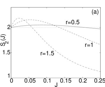
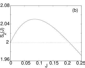
Figure 3:                                                                                                                      (a) Plot of $S_{2}(J)$ versus $J$ for $r=0.5$ (solid line), $r=1$ (dashed line) and $r=1.5$ (-.-.-.) with displacements. Both $S_{2}(J)$ and $J$ are dimensionless. The horizontal dotted line represents $S_{2}(J)=2$.                                                                                           (b) Close-up plot of $S_{2}(J)$ versus $J$ for $r=0.5$ with displacements. The horizontal dotted line represents $S_{2}(J)=2$.

IV.3 Third least significant bits

To show that $|\psi_{\rm CM}\rangle$ violates the bitwise Bell inequality $S_{3}\leq 2$, we now perform a similar calculation to the last subsection’s except that, as the third least significant bit of the numbers $0,1,2,3,8,9,10,11\ldots$ is ‘0’,

$${\rm E}\left[{\bar{a}}_{3}(z_{1}){\bar{b}}_{3}(z_{2})\right] =1-2\times$$

$$\left(\sum_{i={\rm even}}\sum_{j=0}^{3}\sum_{l={\rm odd}}\sum_{s=0}^{3}Pr({\cal N}_{1}=4i+j,{\cal N}_{2}=4l+s|z_{1},z_{2})\right.$$

$$\left.\sum_{i={\rm odd}}\sum_{j=0}^{3}\sum_{l={\rm even}}\sum_{s=0}^{3}Pr({\cal N}_{1}=4i+j,{\cal N}_{2}=4l+s|z_{1},z_{2})\right).$$

Using this result and Eq. (16) to calculate $S_{3}$ as a function of $J$, we obtain the results in Figs 4 (a) and (b) which show bitwise Bell inequality violations. Observe that for certain $J$ and $r$ values, we can simultaneously violate the bitwise Bell inequalities $S_{1}\leq 2$, $S_{2}\leq 2$ and $S_{3}\leq 2$. It is also interesting to note that the violations in Fig. 4 are significantly less than those for the second least significant bits shown in Fig. 3. It is possible that this is due to the fact that groups of four consecutive numbers (eg. 0, 1, 2 and 3) share the same value for their third least significant bits. (For the second least significant bits, only two consecutive numbers share the same value.) Because of this, it may be more difficult for the displacement operations we implement to cause states to ‘flip’ the values of their third least significant bits. In turn, this would mean that it would be more difficult for these operations to generate the sort of interference between previously orthogonal states in $|\psi_{\rm CM}\rangle$ necessary for obtaining Bell violations, thus leading to the smaller violations for the third least significant bits shown in Fig 4.

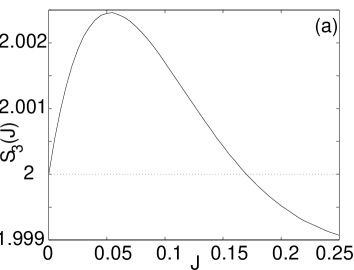
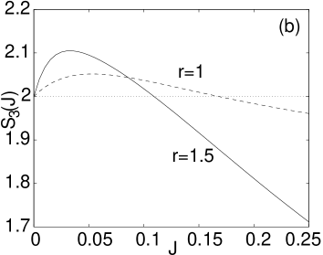
Figure 4:                                                                                                                           (a) Plot of $S_{3}(J)$ versus $J$ for $r=0.5$ with displacements. Both $S_{3}(J)$ and $J$ are dimensionless. The horizontal dotted line represents $S_{3}(J)=2$.                                                                         (b) Plot of $S_{3}(J)$ versus $J$ for $r=1.5$ (solid line) and $r=1$ (dashed line) with displacements. The horizontal dotted line represents $S_{3}(J)=2$.

V Bitwise Bell violation with local squeezing operations

In this subsection we show that unitaries other than displacement operations can yield a bitwise Bell inequality violation for $|\psi_{\rm CM}\rangle$. In particular, we show that squeezing operations applied to the centre-of-mass vibrational states of both sets of ions in the $x$ direction can produce such a violation involving the second least significant bits of ${\cal N}_{1}$ and ${\cal N}_{2}$. These squeezing operations are interesting to consider as they have been practically implemented in ion traps (see, for example, meekhof96 ). Observe, however, that squeezing operations applied to both sets of ions do not produce CHSH inequality violations for the least significant bits in the the binary representations of ${\cal N}_{1}$ and ${\cal N}_{2}$ as squeezing operations are associated with two-phonon creation and annihilation. Thus, they do not cause odd and even phonon number states to change parity and so do not induce the type of interference required for such violations. Throughout this section we assume that $N\geq 2$, so that the measurement scheme involves enough two-level electronic systems to to measure ${\bar{a}}_{2}$ and ${\bar{b}}_{2}$.

Applying the above mentioned squeezing operations to $|\psi_{\rm CM}\rangle$, we obtain

$$|\psi_{S}\rangle=S_{1}(r_{+})S_{2}(r_{-})S_{12}(r)|0,0\rangle,$$ (18)

where $S_{1}$ and $S_{2}$ are single-mode squeezing operators for the centre-of-mass modes of the first and second sets of ions in $|\psi_{\rm CM}\rangle$ in the $x$ direction with real squeezing parameters $r_{+}$ and $r_{-}$. The operator $S_{1}(r_{+})=\exp\left(r_{+}\left(B_{1x}^{(1)\;{\dagger}}\right)^{2}-r_{+}\left(B_{1x}^{(1)}\right)^{2}\right)$, whilst $S_{2}(r_{-})=\exp\left(r_{-}\left(B_{2x}^{(1)\;{\dagger}}\right)^{2}-r_{-}\left(B_{2x}^{(1)}\right)^{2}\right)$. We now determine $Pr_{\rm squeeze}({\cal N}_{1}=n_{1},{\cal N}_{2}=n_{2}|r_{+},r_{-})$, the probability of observing $n_{1}$ and $n_{2}$ centre-of-mass phonons in the $x$ direction for the first and second sets of ions respectively given $S_{1}(r_{+})$ and $S_{2}(r_{-})$ by re-ordering the operators in $S_{1}(r_{+})S_{2}(r_{-})S_{12}(r)|0\rangle_{1}0\rangle_{2}$. The idea for this derived from a calculation in carl that found $\langle{\cal N}_{1}=n_{1},{\cal N}_{2}=n_{2}|\psi_{D}\rangle$ by decomposing and normally ordering the operators in $D_{1}(\alpha)D_{2}(\beta)S_{12}(r)|0\rangle_{1}0\rangle_{2}$.

Decomposing $S_{12}$ in a normally-ordered manner and utilizing the known single-mode squeezing operator decomposition schumaker

$$S_{j}(R) = \exp\bigl{[}-{\rm ln}(\cosh R)(B_{jx}^{(1)\;{\dagger}}B_{jx}^{(1)}+1/2)\bigr{]}\times$$ (19)

$$\exp\bigl{[}\tanh R\cosh^{2}R\left(B_{jx}^{(1)\;{\dagger}}\right)^{2}/2\bigr{]}\times$$

$$\exp\bigl{[}\tanh R\left(B_{jx}^{(1)}\right)^{2}/2\bigr{]},$$

where $j=1,2$, yields

$$|\psi_{S}\rangle = \frac{1}{\sqrt{K}}\times$$ (20)

$$\exp\left(-\ln\cosh_{r+}B_{1x}^{(1)\;{\dagger}}B_{1x}^{(1)}-\ln\cosh_{r-}B_{2x}^{(1)\;{\dagger}}B_{2x}^{(1)}\right)\times$$

$$\exp\left(-\tanh r_{+}\cosh^{2}r_{+}\left(B_{1x}^{(1)\;{\dagger}}\right)^{2}/2\right.$$

$$\left.-\tanh r_{-}\cosh^{2}r_{-}\left(B_{2x}^{(1)\;{\dagger}}\right)^{2}/2\right)\times$$

$$\exp\left(\tanh r_{+}\left(B_{1x}^{(1)}\right)^{2}/2+\tanh r_{-}\left(B_{2x}^{(1)}\right)^{2}/2\right)\times$$

$$\exp(\tanh rB_{1x}^{(1)\;{\dagger}}B_{2x}^{(1)\;{\dagger}})|0,0\rangle,$$

where $K=\cosh^{2}r\cosh r_{+}\cosh r_{-}$.

To determine $Pr_{\rm squeeze}({\cal N}_{1}=n_{1},{\cal N}_{2}=n_{2}|r_{+},r_{-})$ from Eq. (20) we use three operator identities. These identities, which hold for any operators $A$ and $B$ such that $[A,A^{{\dagger}}]=[B,B^{{\dagger}}]=1$ and $[A,B^{{\dagger}}]=[A,B]=0$, are proven in Appendix A and are

$$\exp(c_{1}A^{2})\exp(c_{2}A^{{\dagger}}B^{{\dagger}}) = \exp(c_{2}A^{{\dagger}}B^{{\dagger}})\exp(c_{1}c_{2}^{2}B^{{\dagger}\>2})$$

$$\times \exp(2c_{1}c_{2}AB^{{\dagger}})\;\exp(c_{1}A^{2}),$$

$$\exp(c_{1}A^{2})\exp(c_{2}A^{{\dagger}\>2})=\exp(\frac{c_{2}}{1-4c_{1}c_{2}}A^{{\dagger}\>2})\times$$

$$\exp\bigl{[}\cosh^{-1}\bigl{(}1+\frac{2c_{1}c_{2}}{1-4c_{1}c_{2}}-2c_{1}c_{2}\bigr{)}\{A^{{\dagger}}A+1/2\}\bigr{]}\times$$

$$\exp(\frac{c_{1}}{1-4c_{1}c_{2}}A^{2})$$

$${\rm and}$$

$$\exp(c_{1}A^{{\dagger}}B)\exp(c_{2}B^{{\dagger}\>2})=\exp(c_{2}B^{{\dagger}\>2})\;\exp(2c_{1}c_{2}A^{{\dagger}}B^{{\dagger}})$$

$$\times\exp(c_{1}^{2}c_{2}A^{{\dagger}\>2})\;\exp(c_{1}A^{{\dagger}}B),$$

where $c_{1}$ and $c_{2}$ are complex numbers. Re-ordering terms on the right-hand side of Eq. (20) by applying these identities to $B_{1x}^{(1)}$ and $B_{2x}^{(1)}$ yields

$$|\psi_{S}\rangle = \sqrt{\frac{M}{K}}\times$$

$$\exp\left(-\ln\cosh r_{+}B_{1x}^{(1)\;{\dagger}}B_{1x}^{(1)}-\ln\cosh r_{-}B_{2x}^{(1)\;{\dagger}}B_{2x}^{(1)}\right)\times$$

$$\exp\left[(-1/2\tanh r_{+}\cosh^{2}r_{+}+1/2\tanh r_{-}\tanh^{2}r\right.$$

$$\left.+d_{1}^{2}d_{2})\left(B_{1x}^{(1)\;{\dagger}}\right)^{2}\right]\times$$

$$\exp\left[\left(-1/2\tanh r_{-}\cosh^{2}r_{-}+d_{2})\left(B_{2x}^{(1)\;{\dagger}}\right)^{2}\right)\right.\times$$

$$\left.\exp\left((\tanh r+2d_{1}d_{2})B_{1x}^{(1)\;{\dagger}}B_{2x}^{(1)\;{\dagger}}\right)\right]|0,0\rangle,$$

where $d_{1}=\tanh r\tanh r_{-}$, $d_{2}=d_{4}/1-4d_{3}d_{4}$, $d_{3}=1/2\tanh r_{-}$, $d_{4}=1/2\tanh r_{+}\tanh^{2}r$ and

$$M=\exp\bigl{[}\cosh^{-1}\bigl{(}1+\frac{2d_{3}d_{4}}{1-d_{3}d_{4}}-2d_{3}d_{4}\bigr{)}\bigr{]}.$$

Calculating $Pr_{\rm squeeze}({\cal N}_{1}=n_{1},{\cal N}_{2}=n_{2}|r_{+},r_{-})$ using the right-hand side of Eq. (V), we arrive at

$$Pr_{\rm squeeze}({\cal N}_{1}=n_{1},{\cal N}_{2}=n_{2}|r_{+},r_{-}) = f(n_{1},n_{2})\times$$

$$\left|\sqrt{\frac{M}{K}}\sqrt{n_{1}!n_{2}!}\cosh^{-n_{1}}r_{+}\cosh^{-n_{2}}r_{-}e_{+}^{n_{1}/2}e_{-}^{n_{2}/2}\right.$$

$$\left.\sum_{j=0+f,2+f,4+f\ldots}^{{\rm min}(n_{1},n_{2})}(\frac{e_{\rm two}}{\sqrt{e_{+}e_{-}}})^{j}\frac{1}{j!((n_{1}-j)/2)!((n_{2}-j)/2)!}\right|^{2},$$

where

$$f(n_{1},n_{2})=\left\{\begin{array}[]{cc}0&,n_{1}+n_{2}=\>{\rm even}\\ 1&,n_{1}+n_{2}=\>{\rm odd},\end{array}\right.$$ (26)

$e_{+}=-1/2\tanh r_{+}\cosh^{2}r_{+}+1/2\tanh r_{-}\tanh^{2}r+d_{1}^{2}d_{2}$, $e_{-}=-1/2\tanh r_{-}\cosh^{2}r_{-}+d_{2}$ and $e_{\rm two}=\tanh r+2d_{1}d_{2}$. Observe that it was crucial to re-order the operators on the right-hand side of Eq. (20) in arriving at Eq. (LABEL:final) as if we did not then we would have had to deal with infinitely many terms contributing to $P_{\rm squeeze}({\cal N}_{1}=n_{1},{\cal N}_{2}=n_{2}|r_{+},r_{-})$. The reason for this is that the right-hand side of Eq. (20) contains annihilation operators to the left of creation operators for the same mode. As a consequence, for example, upon considering power series expansions of the exponentials in this equation we have contributions to $|0,0\rangle$ from terms in which we first create $X$ centre-of-mass phonons, where $X=1,2,3\ldots$, by applying $\left(B_{1x}^{(1){\dagger}}\right)^{X}$, and then annihilate them by applying $\left(B_{1x}^{(1)}\right)^{X}$ to $\left(B_{1(x)}^{(1)\;{\dagger}}\right)^{X}|0,0\rangle$. Given that $X$ can be any natural number, it follows that, to determine $Pr_{\rm squeeze}({\cal N}_{1}=0,{\cal N}_{2}=0|r_{+},r_{-})$ using Eq. (20), we seem to need to consider infinitely many contributing terms. In contrast, the only annihilation operators that appear to the left of creation operators in the right-hand side of Eq. (V) are present in terms containing number operators. These do not increase or decrease the number of centre-of-mass phonons when applied to a state and so their presence does not cause infinitely many terms to contribute to $P_{\rm squeeze}({\cal N}_{1}=n_{1},{\cal N}_{2}=n_{2}|r_{+},r_{-})$, thus making the calculation of $P_{\rm squeeze}({\cal N}_{1}=n_{1},{\cal N}_{2}=n_{2}|r_{+},r_{-})$ tractable. Using $Pr_{\rm squeeze}({\cal N}_{1}=n_{1},{\cal N}_{2}=n_{2}|r_{+},r_{-})$ to calculate CHSH correlations in a similar manner to that used to determine $Pr({\cal N}_{1}=n_{1},{\cal N}_{2}=n_{2}|z_{1},z_{2})$ in Subsection IV.2, we find that the CHSH inequality is violated, as illustrated in Figs 5 (a) and (b) which show $S_{2}$ as a function of $J$ for $r=0.5$, $r=1$ and $r=1.25$.

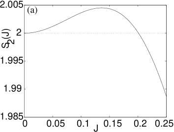
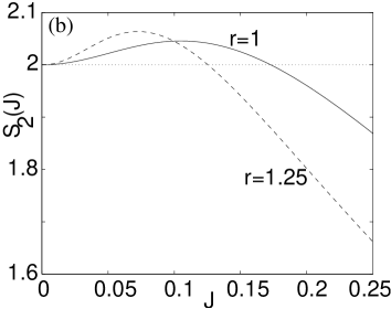
Figure 5:
(a) Plot of $S_{2}(J)$ versus $J$ for $r=0.5$ with local squeezing operations. Both $S_{2}(J)$ and $J$ are dimensionless. The horizontal dotted line represents the equation $S_{2}(J)=2$.
(b) Plot of $S_{2}(J)$ versus $J$ for $r=1$ (solid line) and $r=1.25$ (dashed line) with local squeezing operations. The horizontal dotted line represents the equation $S_{2}(J)=2$.

VI Discussion

Though this paper’s results are related to those in larrson03 , they differ from larrson03 ’s results in a number of ways. First, motivated by the comment in larrson03 that the formulation of a more practical measurement scheme to measure larrson03 ’s Bell inequalities was desirable, we arguably proposed such a scheme (at least for the least, second least and third least significant bits of ${\cal N}_{1}$ and ${\cal N}_{2}$) which centred on transferring the centre-of-mass vibrational state of group of trapped ions to the internal states of a group of electrons. Second, we violated inequalities similar to those in larrson03 using vastly different schemes to those in larrson03 . In larrson03 the measurements made in violating the inequalities were pseudo-spin measurements along varying axes in a two-dimensional plane. In contrast, we measured a pseudo-spin based observable in a single direction and obtain violations by applying a range of displacements and squeezing operations to sets of $N$ ions.

Aside from extending work in larrson03 , the Bell violations in Section IV are noteworthy as they are similar to those attainable in so-called hyper-entangled states kwiat97 . These are states in which more than four degrees of freedom are entangled, such as a two-photon state with polarisation, energy and momentum entanglement (each particle has a polarisation, an energy and a momentum degree of freedom participating in the entanglement). As a consequence, hyper-entangled states can violate multiple Bell inequalities involving, collectively, five or more degrees of freedom. The Bell violations in Section IV are similar to those achievable in hyper-entangled states as the violations in Section IV involve violating three Bell inequalities involving six degrees of freedom, namely the three least significant bits of both ${\cal N}_{1}$ and ${\cal N}_{2}$. One reason why this connection is interesting is that indirect evidence suggests kwiat97 (pp. 2179-81) that some hyper-entangled states may be able to perform certain interesting quantum information processing. This, in turn, suggests that $|\psi_{\rm CM}\rangle$ may also be able to perform such feats.

Though we only demonstrated bitwise Bell violations for the three least significant bits of ${\cal N}_{1}$ and ${\cal N}_{2}$ others, presumably, also exist for the fourth, fifth, sixth etc. least significant bits. However, the calculations required to demonstrate these violations were not performed as calculating $S_{y}$ becomes increasingly difficult as $y$ increases due to the presence of more and more complicated spreads of centre-of-mass number states sharing the same value for the $y^{\rm th}$ bit. An example of this increased complication can be seen by observing the fact that Eq. (LABEL:joint_correlation) ($y=2$) is simpler than Eq. (IV.3) ($y=3$).

An alternate approach we could have taken to investigating $|\psi_{\rm CM}\rangle$’s nonclassical correlations would have been to see what quantum information processing tasks this state’s correlations could be used to perform. However, one complication with this is that the $2N$ systems in the total physical system described by $|\psi_{\rm CM}\rangle$ are not qubits but instead are infinite-dimensional harmonic oscillators. Because of this, we cannot directly consider if this state is useful in helping to implement well-known quantum protocols for qubits. In spite of this difficulty, however, a recent result showing that certain Bell violations imply the existence of quantum communication complexity protocols superior to any classical ones brukner02 may be useful in manifesting $|\psi_{\rm CM}\rangle$’s nonclassical correlations. In particular, it may allow us to readily show that Section IV’s Bell violations imply that $|\psi_{\rm CM}\rangle$ could be employed to perform such quantum protocols.

Yet another approach that could be taken to illustrate the nonclassicality of $|\psi_{\rm CM}\rangle$ is to use entanglement witnesses terhal00 . An entanglement witness $W$ for the entangled state $\rho$ is an operator such that $Tr(\rho W)<0$ and $Tr(\sigma W)>0$ whenever $\sigma$ is a separable state. This approach would involve identifying suitable operators $W$ and then applying them to $|\psi_{\rm CM}\rangle$. We acknowledge that it may be a useful approach to try, however, we have not explored it.

How feasible are the system and measurement scheme we have discussed? To reiterate, first, the system involving the parametric oscillators feeding into two cavities within which lie ion traps containing $N$ ions does not seem to be infeasible. This is because, as stated earlier, optical cavities and nondegenerate optical parametric amplifiers have been widely realized in laboratories for some time. In addition, experiments in which a single harmonically trapped ion has been placed within an optical cavity have been conducted mundt02 . Another factor consistent with the potential feasibility of the system considered is that the entangled state $|\psi_{\rm CM}\rangle$ can be created, to a good approximation, on a timescale far shorter than that of the vibrational decoherence for the ions. Finally, displacement and squeezing operations on trapped ions have been realised in meekhof96 via shining laser beams on the ions.

To conclude, following on from larrson03 we have presented Bell inequalities that reveal certain nonclassical correlations in $|\psi_{\rm CM}\rangle$. In particular, these correlations are between bits in the binary representations of ${\cal N}_{1}$ and ${\cal N}_{2}$ that violate three bitwise inequalites. We have also presented a bitwise Bell violation for $|\psi_{\rm CM}\rangle$ involving local squeezing operations.

Appendix A: Operator identities using Lie algebras

In this appendix we prove the identities

$$\exp(c_{1}A^{2})\exp(c_{2}A^{{\dagger}}B^{{\dagger}}) = \exp(c_{2}A^{{\dagger}}B^{{\dagger}})\exp(c_{1}c_{2}^{2}B^{{\dagger}\>2})$$

$$\times \exp(2c_{1}c_{2}AB^{{\dagger}})\;\exp(c_{1}A^{2}),$$

$$\exp(c_{1}A^{2})\exp(c_{2}A^{{\dagger}\>2})=\exp(\frac{c_{2}}{1-4c_{1}c_{2}}A^{{\dagger}\>2})\times$$

$$\exp\bigl{[}\cosh^{-1}\bigl{(}1+\frac{2c_{1}c_{2}}{1-4c_{1}c_{2}}-2c_{1}c_{2}\bigr{)}\{A^{{\dagger}}A+1/2\}\bigr{]}\times$$

$$\exp(\frac{c_{1}}{1-4c_{1}c_{2}}A^{2})$$

$${\rm and}$$

$$\exp(c_{1}A^{{\dagger}}B)\exp(c_{2}B^{{\dagger}\>2})=\exp(c_{2}B^{{\dagger}\>2})\;\exp(2c_{1}c_{2}A^{{\dagger}}B^{{\dagger}})$$

$$\times\exp(c_{1}^{2}c_{2}A^{{\dagger}\>2})\;\exp(c_{1}A^{{\dagger}}B),$$

where the $c_{1}$ and $c_{2}$ are $c$-number co-efficients and $A$ and $B$ are bosonic centre-of-mass annihilation operators for two non-interacting systems for which $[A,A^{{\dagger}}]=[B,B^{{\dagger}}]=1$. We do this using the Baker-Campbell-Hausdorff (BCH) formula varadarajan84 , a technique that has been called the differential-equation approach schumaker ; truax88 and the fact that SU(1,1) has a two-dimensional matrix representation.

The BCH formula is varadarajan84 (p. 118)

$$\exp({\cal A})\exp({\cal B}) =$$

$$\exp\bigl{(}{\cal A}+{\cal B}+1/2[{\cal A},{\cal B}]+1/12\{[{\cal A},[{\cal A},{\cal B}]]+[[{\cal A},{\cal B}],{\cal B}]\}$$

$$+1/48\{[{\cal B},[{\cal A},[{\cal B},{\cal A}]]]+[[[{\cal A},{\cal B}],{\cal A}],{\cal B}]\}+\ldots\bigr{)},$$

where ${\cal A}$ and ${\cal B}$ are abitrary operators. We use it in proving Eqs (LABEL:identity1) and (LABEL:identity3) by employing it to convert their left-hand sides into a single exponential each. Next, we convert these single exponentials to the normally-ordered products of exponentials on the right-hand sides of Eqs (LABEL:identity1) and (LABEL:identity3) using the differential-equation approach, which we now explain. This approach disentangles or decomposes a single exponential with a sum in its exponent, into a product of a number of exponentials in the following manner: First, we multiply the exponent of the single exponential by a parameter $t$. Next, we equate the single exponential with this extra factor of $t$ in its exponent to a product of exponentials for which each exponent is some unknown function of $t$ multiplied by a generator of a certain Lie group. The group is the same for all exponents and is one for which all terms in the exponent of the original single exponential are some constant multiplied by a generator of the group. In addition, each generator appears precisely once in the product of exponentials. To give an example, consider the single exponential $\exp(c_{1}A^{{\dagger}\>2}+c_{2}A^{2})$. Noting that $A^{2}$ and $A^{{\dagger}\>2}$ are generators of SU(1,1), we multiply $c_{1}A^{{\dagger}\>2}+c_{2}A^{2}$ by $t$ and equate $\exp\left((c_{1}A^{{\dagger}\>2}+c_{2}A^{2})t\right)$ to the following product of exponentials:

$$\exp\left(f_{1}(t)A^{{\dagger}\>2}\right)\exp\left(f_{2}(t)(A^{{\dagger}}A+1/2)\right)\exp\left(f_{2}(t)A^{2}\right).$$ (31)

Observe that in expression (31) that each exponent is the product of an unknown function and a generator of $SU(1,1)$. Furthermore, each of $SU(1,1)$’s generators appears exactly once. Returning to the general case, finally, we calculate the unknown functions of $t$, and so complete the process of disentangling the single exponential, by differentiating both sides of the equation equating the single exponential with the extra factor of $t$ in its exponent to the product of exponentials with respect to $t$, multiplying both sides from the right by the inverse of the single exponential and, lastly, equating operator coefficients on both sides. The paper truax88 contains a detailed example in which the differential-equation approach is used.

Using the BCH formula on the left-hand side of Eq. (LABEL:identity1) yields

$$\exp(c_{1}A^{2})\exp(c_{2}A^{{\dagger}}B^{{\dagger}})$$ (32)

$$=\exp(c_{1}A^{2}+c_{2}A^{{\dagger}}B^{{\dagger}}+c_{1}c_{2}AB^{{\dagger}}+\frac{c_{1}c_{2}^{2}}{6}B^{{\dagger}\>2}).$$

Noting that $\{A^{{\dagger}}B^{{\dagger}},A^{2},AB^{{\dagger}},B^{{\dagger}\>2}\}$ form a Lie algebra, we use the differential-equation approach on the right-hand side of Eq. (32) to know that there exists a normally-ordered decomposition such that

$$\exp\bigl{[}(c_{1}A^{2}+c_{2}A^{{\dagger}}B^{{\dagger}}+c_{1}c_{2}AB^{{\dagger}}+\frac{c_{1}c_{2}^{2}}{6}B^{{\dagger}\>2})t\bigr{]}$$

$$=\exp(f_{1}(t)A^{{\dagger}}B^{{\dagger}})\exp(f_{2}(t)B^{{\dagger}\>2})\times$$

$$\exp(f_{3}(t)B^{{\dagger}}A)\exp(f_{4}(t)A^{2})$$

$$=U,$$

where $f_{1}$, $f_{2}$, $f_{3}$ and $f_{4}$ are functions we now determine. Differentiating both sides of Eq. (Appendix A: Operator identities using Lie algebras) with respect to t and then multiplying from the right by $U^{-1}$ yields

$$c_{1}A^{2}+c_{2}A^{{\dagger}}B^{{\dagger}}+c_{1}c_{2}AB^{{\dagger}}+\frac{c_{1}c_{2}^{2}}{6}B^{{\dagger}\>2}$$

$$\;\;=\;\;{\dot{f}}_{1}A^{{\dagger}}B^{{\dagger}}+{\dot{f}}_{2}\;e^{f_{1}A^{{\dagger}}B^{{\dagger}}}\;B^{{\dagger}\>2}\;e^{-f_{1}A^{{\dagger}}B^{{\dagger}}}\;$$

$$+\;{\dot{f}}_{3}\;e^{f_{1}A^{{\dagger}}B^{{\dagger}}}\;e^{f_{2}B^{{\dagger}\>2}}\;B^{{\dagger}}a\;e^{-f_{2}B^{{\dagger}\>2}}\;e^{-f_{1}A^{{\dagger}}B^{{\dagger}}}\;\;$$

$$+\;\;{\dot{f}}_{4}\;e^{f_{1}A^{{\dagger}}B^{{\dagger}}}\;e^{f_{2}B^{{\dagger}\>2}}\;e^{f_{3}B^{{\dagger}}A}\;B^{{\dagger}\>2}\;e^{-f_{3}B^{{\dagger}}A}$$

$$\times\;e^{-f_{2}B^{{\dagger}\>2}}\;e^{-f_{1}A^{{\dagger}}B^{{\dagger}}}$$

where ${\dot{f}_{i}}$ denotes $\partial f_{i}/\partial t$. Using the identity merzbacher61 (p. 162)

$$\exp({\cal A}){\cal B}\exp(-{\cal A})={\cal B}+[{\cal A},{\cal B}]+1/2![{\cal A},[{\cal A},{\cal B}]]+\ldots,$$ (35)

where ${\cal A}$ and ${\cal B}$ are arbitrary operators, on the right-hand side of Eq. (Appendix A: Operator identities using Lie algebras) produces

$$c_{1}A^{2}+c_{2}A^{{\dagger}}B^{{\dagger}}+c_{1}c_{2}AB^{{\dagger}}+\frac{c_{1}c_{2}^{2}}{6}B^{{\dagger}\>2}$$ (36)

$$={\dot{f}}_{1}A^{{\dagger}}B^{{\dagger}}+{\dot{f}}_{2}B^{{\dagger}\>2}+{\dot{f}}_{3}(B^{{\dagger}}A-f_{1}B^{{\dagger}\>2})$$

$$+{\dot{f}}_{4}(A^{2}-2f_{1}B^{{\dagger}}A+f_{1}^{2}B^{{\dagger}\>2}).$$

Upon equating operator coefficients we arrive at four coupled differential equations for the $f_{i}^{\prime}s$. Solving these and setting t=1 yields

$$\exp(c_{1}A^{2}+c_{2}A^{{\dagger}}B^{{\dagger}}+c_{1}c_{2}AB^{{\dagger}}+\frac{c_{1}c_{2}^{2}}{6}B^{{\dagger}\>2})$$ (37)

$$\exp(c_{2}A^{{\dagger}}B^{{\dagger}})\;\exp(c_{1}c_{2}^{2}B^{{\dagger}\>2})\;\exp(2c_{1}c_{2}B^{{\dagger}}A)\;\exp(c_{1}A^{2}).$$

Recalling that

$$\exp(c_{1}A^{2}+c_{2}A^{{\dagger}}B^{{\dagger}}+c_{1}c_{2}AB^{{\dagger}}+\frac{c_{1}c_{2}^{2}}{6}B^{{\dagger}\>2})=$$ (38)

$$\exp(c_{1}A^{2})\exp(c_{2}A^{{\dagger}}B^{{\dagger}})$$

we arrive at Eq. (LABEL:identity1). The identity in Eq. (LABEL:identity3) can be obtained via a very similar calculation to that which we have just performed.

To prove Eq. (Appendix A: Operator identities using Lie algebras), we first note that $A^{2}$ and $A^{{\dagger}\>2}$ are generators of the Lie group SU(1,1). Related to this group, it is known that schumaker

$$\exp(c_{1}A^{2})\exp(c_{3}(A^{{\dagger}}A+1/2))\exp(c_{2}A^{{\dagger}\>2})$$

$$=\exp(\beta_{1}(\{c_{i}\})A^{{\dagger}\>2})\exp(\beta_{2}(\{c_{i}\})(A^{{\dagger}}A+1/2))$$

$$\hskip 9.95863pt\exp(\beta_{3}(\{c_{i}\})A^{{\dagger}\>2}),$$ (39)

where $\beta_{1}$, $\beta_{2}$ and $\beta_{3}$ are, as yet, unknown functions. Noting that these functions are only determined by the commutation-relation structure of SU(1,1)’s generators, we follow schumaker and replace $A^{{\dagger}\>2}$, $(A^{{\dagger}}A+1/2)$ and $A^{2}$ by two-dimensional matrices with identical commutation relations. This leads us to making the following transformations: $A^{{\dagger}\>2}\rightarrow 2\sigma_{+}$, $A^{2}\rightarrow-2\sigma_{-}$ and $A^{{\dagger}}A+1/2\rightarrow\sigma_{z}$, where

$$\sigma_{+}=\left\{\begin{array}[]{ll}0&1\\ 0&0\\ \end{array}\right\},$$ (42)

$$\sigma_{-}=\left\{\begin{array}[]{ll}0&0\\ 1&0\\ \end{array}\right\}$$ (45)

and

$$\sigma_{z}=\left\{\begin{array}[]{ll}1&0\\ 0&-1\\ \end{array}\right\}.$$ (48)

Upon doing this, and setting $c_{3}=0$, the left-hand side of Eq. (Appendix A: Operator identities using Lie algebras) becomes

$$\exp(-2c_{1}\sigma_{-})\exp(2c_{2}\sigma_{+}) = \left\{\begin{array}[]{ll}1&2c_{2}\\ -2c_{1}&1-4c_{1}c_{2}\\ \end{array}\right\}$$ (51)

whilst the right-hand side transforms to

$$\exp(\beta_{1}2\sigma_{+})\exp(\beta_{2}\sigma_{z})\exp(-\beta_{3}2\sigma_{-})$$

$$=\left\{\begin{array}[]{ll}P-4\beta_{1}\beta_{3}M&2\beta_{1}M\\ -2\beta_{3}M&M\\ \end{array}\right\},$$ (54)

where $P=\cosh\beta_{2}+\sinh\beta_{2}$ and $M=\cosh\beta_{2}-\sinh\beta_{2}$. Equating matrix elements on the right-hand sides of Eqs (51) and (Appendix A: Operator identities using Lie algebras) leads to

$$\beta_{1} = c_{2}/(1-4c_{1}c_{2})$$

$$\beta_{2} = \cosh^{-1}\bigl{(}1+2c_{1}c_{2}/(1-4c_{1}c_{2})-2c_{1}c_{2}\bigr{)}$$

$${\rm and}$$

$$\beta_{3} = c_{1}/(1-4c_{1}c_{2})$$ (55)

and hence to Eq. (Appendix A: Operator identities using Lie algebras).

References

- (1) M. A Nielsen and I. L. Chuang, Quantum Computation and Quantum Information (Cambridge University Press, Cambridge, 2000);
- (2) J. Preskill, Physics 229: Advanced Mathematical Methods of Physics — Quantum Computation and Information. California Institute of Technology, 1998. URL: http://www.theory.caltech.edu/people/preskill/ph229/
- (3) C. H. Bennett, G. Brassard, C. Crépeau, R. Jozsa, A. Peres, and W. K. Wootters, Phys. Rev. Lett. 70 (1993) 1895.
- (4) C. H. Bennett and S. W. Wiesner Phys. Rev. Lett. 69, 2881 (1992).
- (5) J. S. Bell, Physics 1, 195 (1964).
- (6) J. F. Clauser and A. Shimony, “Bell’s theorem: experimental tests and implications” Rep. on Prog. in Physics 41, 1881 (1978).
- (7) J. F. Clauser. M. A. Horne, A. Shimony, and R. A. Holt, Phys. Rev. Lett. 49, 1804 (1969).
- (8) D. M. Greenberger, M. A. Horne, and A. Zeilinger, in Bell’s Theorem, Quantum Theory and Conceptions of the Universe, edited by M. Kafatos (Kluwer Academic, Dordrecht, 1989) p.69; D. M. Greenberger et al., Am. J. Phys. 58, 1131 (1990).
- (9) N. D. Mermin, Phys. Rev. Lett. 65, 1838 (1990).
- (10) N. D. Mermin, Phys. Rev. D 22, 356 (1980).
- (11) A. Peres, Found. Phys. 29, 589 (1999).
- (12) R. F. Werner, Phys. Rev. A 61, 062102 (2000).
- (13) J.-Ä. Larrson, Phys. Rev. A 67, 022108 (2003).
- (14) K. Banasek and K. Wodkiewicz, Phys. Rev. A 58, 4345 (1998).
- (15) K. Banasek and K. Wodkiewicz, Phys. Rev. Lett. 82, 2009 (1999).
- (16) K. Banasek and K. Wodkiewicz, Acta Phys. Slov. 49, 491 (1999).
- (17) Z. B. Chen, J. W. Pan, G. Hou and Y. D. Zhang, Phys. Rev. Lett. 88, 040406 (2002).
- (18) G. Gour, F. C. Khanna, A. Mann, M. Revzen, e-print quant-ph/0308063.
- (19) W. Dür, G. Vidal, and J. I. Cirac, Phys. Rev. A 62 062314 (2000).
- (20) C. Brukner et al. quant-ph/0210114.
- (21) Z. Y. Ou, S. F. Pereira, H. J. Kimble, and K. C. Peng, Phys. Rev. Lett. 68, 3663 (1992).
- (22) Z. Y. Ou, S. F. Pereira, and H. J. Kimble, Photophys. Laser Chem. 55, 265 (1992).
- (23) H. J. Kimble, in Fundamental Systems in Quantum Optics, Proceedings of the Les Houches Summer School of Theoretical Physics, Session LIII, Les Houches, 1990, edited by J. Dalibard et al. (Elsevier, New York, 1992).
- (24) See, for example, M. G. Raizen et al., Phys. Rev. A 45, 6493 (1992), H. Walther, Adv. At. Mod. Opt. Phys. 32, 379 (1994) and D. J. Wineland et al., J. Res. Natl Inst. Stan. 103, 259 (1998).
- (25) D. V. James, App. Phys. B 66, 181 (1998).
- (26) A. S. Parkins and H.J. Kimble, J. Opt. B: Quantum Semiclass. Opt. 1 496 (1999).
- (27) A. B. Mundt et al., e-print quant-ph/0202112.
- (28) A. S. Parkins and H. J. Kimble, Phys. Rev. A 61, 052104 (2000).
- (29) J. Ye, D. W. Vernooy and H. J. Kimble, Phys. Rev. Lett. 83, 4987 (1999).
- (30) C. W. Gardiner and M. J. Collett, Phys. Rev. A 31, 3761 (1985).
- (31) A. S. Parkins and E. Larsabal, Phys. Rev. A 63, 012304 (2001).
- (32) C. D’Helon and G. J. Milburn, Phys. Rev. A 54, 5141 (1996).
- (33) D. Heinzen, J. J. Bolinger, and D. J. Wineland, Phys. Rev. A 41, 2295 (1990).
- (34) C. Munroe et al. Science 272, 1131 (1996).
- (35) D. M. Meekhof, C. Monroe, B. E. King, W. M. Itano, and D. J. Wineland, Phys. Rev. Lett. 76, 1796 (1996).
- (36) C. M. Caves, C. Zhu, G. J. Milburn, and W. Schleich, Phys. Rev. A 43 3854 (1991).
- (37) Numerical errors were induced in our values for as, practically, we had to truncate the sums in over and in Eq. (16) at finite values. These errors were estimated by truncating the sums in at a number of increasing and values and then seeing to what extent varied upon doing so.
- (38) B. L. Schumaker and C. M. Caves, Phys. Rev. A 31, 3093 (1986).
- (39) P. Kwiat, J. Mod. Optics 44, 2173 (1997).
- (40) B. Terhal, Phys. Lett. A, 271 319 (2000).
- (41) V.S. Varadarajan, Lie Groups, Lie Algebras and their Representations (Springer-Verlag, New York, 1984).
- (42) R. D. Truax, Phys. Rev. D 31, 1988 (1985).
- (43) E. Merzbacher, Quantum Mechanics (John Wiley, 1961).