Scalable Superconducting Architecture for Adiabatic Quantum Computation

Abstract

A scalable superconducting architecture for adiabatic quantum computers is proposed. The architecture is based on time-independent, nearest-neighbor interqubit couplings: it can handle any problem in the class NP even in the presence of measurement errors, noise, and decoherence. The implementation of this architecture with superconducting persistent-current qubits and the natural robustness of such an implementation to manufacturing imprecision and decoherence are discussed.

Adiabatic quantum computation Farhi et al. (2001) is an approach to solving computational problems of the complexity class NP Garey and Johnson (1979) via energy minimization. In particular, by exploiting the ability of coherent quantum systems to follow adiabatically the ground state of a slowly changing Hamiltonian, it aims to bypass the many separated local minima that occur in difficult minimization problems. Adiabatic quantum computation is of theoretical interest because it provides a straightforward, non-oracular way to pose class NP problems on a quantum computer. To date, most research on it focuses on ascertaining its time complexity Farhi et al. (2001); Childs et al. (2002a); Hogg (2003); van Dam et al. (2001); Farhi et al. (2002). However, it is also of practical interest because encoding a quantum computation in a single eigenstate, the ground state, offers intrinsic protection against dephasing and dissipation Childs et al. (2002b); Roland and Cerf (2003).

In this Letter, we present a scalable superconducting architecture for adiabatic quantum computation that can handle any class NP problem. It requires neither efficient qubit measurements, nor interqubit couplings beyond nearest neighbors, nor couplings that vary during the course of the computation. We also discuss how to implement this architecture specifically with superconducting persistent-current (PC) qubits Mooij et al. (1999); Orlando et al. (1999), which constitute a promising approach to lithographable solid-state qubits. We show that the proposed architecture is robust against manufacturing imprecision, and we estimate the maximum size problem the architecture could support if it were implemented with existing PC qubits at dilution refrigerator temperatures of 10 mK. This maximum stems from the condition that the environment must not excite the computer from its ground state. A simple Boltzmann factor argument implies that a 10 mK temperature limits the PC qubit architecture to NP problem instances of $O(50)$ bits. However, advances in cryogenics or in fabricating PC qubits from higher-$T_{c}$ materials could raise this limit by 1 or 2 orders of magnitude.

Background: In adiabatic quantum computation, one encodes the answer(s) to a hard constrained minimization problem in the ground state(s) of a suitable Hamiltonian $H$ whose local couplings ensure its ground state(s) satisfy the problem’s constraints. One initiates the system in the ground state of another Hamiltonian $H_{0}$ chosen so its ground state is quickly reachable simply by cooling. One then adiabatically deforms $H_{0}$ into $H$ by applying a time-dependent Hamiltonian $H(t)$ such that $H(0)=H_{0}$ and $H(T)=H$. The adiabatic approximation holds as long $H(t)$ possesses at all times a spectral gap $\Delta(t)$ between its instantaneous ground $|\psi_{0}(t)\rangle$ and excited states $|\psi_{n}(t)\rangle$ such that $\frac{\langle\psi_{0}(t)|dH^{2}(t)/dt|\psi_{0}(t)\rangle}{\Delta^{2}(t)}\ll 1$. The question of whether adiabatic quantum computation has polynomial or exponential time complexity is thus determined by whether the minimum gap $\Delta_{\min}(n)$ shrinks polynomially or exponentially in the number of qubits $n$.

It is still unknown what speedup adiabatic quantum computation offers in general over classical energy minimization algorithms. Numerical investigations of hard instances of NP-complete problems Farhi et al. (2001); Childs et al. (2002a); Hogg (2003) suggest that $\Delta_{\min}(n)=O(n^{-1})$, at least typically, and thus adiabatic quantum computation may provide for all practical purposes an exponential speedup on NP-complete problems over all known classical algorithms. However, quantitatively bounding the minimum gaps for adiabatic algorithms for NP-complete problem instances is apparently as hard as solving the actual NP-complete instances themselves. Thus, these numerical investigations have been confined to problems with $\lesssim 30$ qubits. Ref. van Dam et al. (2001) constructs a problem that takes exponential time for a simple version of the adiabatic algorithm. However, Ref. Farhi et al. (2002) shows that alternative versions of the adiabatic algorithm solve the problem of van Dam et al. (2001) in polynomial time, and presents a problem for which simulated annealing provably takes exponential time yet adiabatic quantum computation takes only polynomial time. Definitively establishing the efficiency of the adiabatic algorithm for large problem instances may thus have to await the actual construction of adiabatic quantum computers of the sort described here.

Layout Requirements: By definition, a scalable programmable architecture for adiabatic quantum computing possesses some regular geometrical layout of switchable pairwise couplings on $m$ nodes that can efficiently encode problem Hamiltonians corresponding to any instance of some desired class of energy minimization problems up to $n\leq m$ bits in size. To have the maximum flexibility in the problems one can pose and to exploit the maximum potential power of adiabatic quantum computation, the binary constraint problem the architecture naturally poses should be NP-complete, and the architecture should readily pose instances of it that are truly difficult for all known classical heuristics. Additionally, present experimental constraints make it highly desirable to have couplings that neither extend beyond nearest neighbors nor vary in time beyond possibly switching between a full strength “on” state and a much reduced strength “off” state before computation begins so as to allow programming of the desired problem.

An architecture meeting these requirements naturally follows from the fact Barahona (1982) that calculating the ground state of an antiferromagnetically coupled Ising model in a uniform magnetic field is isomorphic to solving the NP-complete graph theory problem Max Independent Set (MIS), which is the problem of finding for a graph $G=(V,E)$ the largest subset $S$ of the vertices $V$ such that no two members of $S$ are joined by an edge from $E$. Interqubit couplings may be laid on a single plane and kept to a modest number since MIS remains NP-complete even in the ostensibly simple, topologically uniform case of degree-3 planar graphs, i.e., graphs that can be drawn in a plane without any edges crossing and in which every vertex is connected to exactly 3 others Garey et al. (1976).

The isomorphism takes a particularly simple form in this case: the MISs of a degree-3 planar graph $G=(V,E)$ are the ground states of an Ising model with spins on vertices $V$, equal strength antiferromagnetic couplings along some desired axis $\hat{n}$ on edges $E$, placed in a uniform applied magnetic field also along $\hat{n}$:

$$H\propto\sum_{i\in V}\sigma_{\hat{n}}^{(i)}+\sum_{i,j\in E}\sigma_{\hat{n}}^{(i)}\sigma_{\hat{n}}^{(j)}$$ (1)

In regard to the requirement of posing truly hard problem instances, note that the most efficient classical approximation algorithm known for MIS restricted to planar graphs has a cost that grows exponentially in the desired accuracy. Specifically, the cost to obtain an approximate MIS of a planar graph with $n$ vertices that has a cardinality which is at least $\frac{k}{k+1}$ of the true MIS’s cardinality is $O(8^{k}kn)$, and is thus impractical once one desires $\gtrsim 90\%$ accuracy ($k\gtrsim 9$) Baker (1994).

The requirements of nearest neighbor couplings, maximum uniformity, and time-independent control can be met via the layout depicted in Fig. 1: a triangular lattice with qubits at its vertices and nearest-neighbor ferro- or antiferromagnetic couplings on its edges. To allow programmability, that is, to embed an arbitrary degree-3 planar graph in this triangular lattice, each coupling is switchable and moreover the magnetic field on each qubit is individually controllable so as to allow one to create “dummy” qubits that possess no single qubit Hamiltonian and act simply to propagate a coupling. (Triangular lattices make it especially easy to embed degree-3 planar graphs, but lattices with a lower node degree, such as square or hexagonal lattices, would also suffice.)

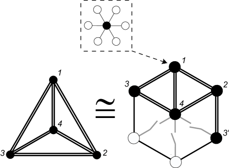
Figure 1: Schematic of the embedding of the simplest degree-3 planar graph (left) into the architecture (right). The architecture is built on a triangular lattice with qubits at its vertices (schematically denoted by filled circles if possessing a Zeeman term and thus denoting a graph vertex, open circles if not and thus denoting a dummy vertex that serves only to propagate a coupling) and switchable nearest-neighbor couplings on its edges (schematically denoted by black double lines if antiferromagnetic and switched on, black single lines if ferromagnetic and switched on, and gray broken lines if switched off). This allows an arbitrary degree-3 planar graph to be embedded efficiently within the lattice, as can be seen in how the Qubit $\#3$ of the graph is ferromagnetically coupled via dummies to a partner $\#3^{\prime}$ so that is a nearest neighbor of $\#2$. Inset: To compensate for measurement errors, the logical qubits in the architecture (denoted by the larger circles) are actually ferromagnetically coupled clusters of physical qubits (smaller circles). For example, as depicted above, one could ferromagnetically couple 6 dummies to each physical computational qubit and thus essentially compensate for measurement errors by a classical 7-bit repetition code. The ferromagnetic couplings in such redundant clusters need not be switchable.

Implementation with PC Qubits: Fig. 2A depicts the specific PC qubit circuit we shall consider here. Ref. Orlando et al. (1999) explains the rationale underlying its design and its canonical quantization. For our purposes, the pertinent result of Ref. Orlando et al. (1999) is that in the regime of sufficiently low temperatures ($T\lesssim 10^{-3}E_{J}\approx 30$ mK for our parameters) and frustrations that make all the minima of the junctions’ potential energies nearly equal ($0.485\Phi_{0}\lesssim f^{\mathrm{bot}}+\frac{1}{2}f^{\mathrm{top}}\lesssim 0.515\Phi_{0})$, the circuit is accurately described by a truncated 2-level qubit Hamiltonian that has a simple, readily tunable form. Specifically, numerical analysis shows for realistic parameters of $E_{J}/E_{C}=80,\beta=0.8,\gamma=0.02$ and frustrated at $f^{\mathrm{top(bot)}}=\left[0.330+\delta^{\mathrm{top(bot)}}\right]\Phi_{0}$ yields an effective qubit Hamiltonian $H_{Q}$:

$$\frac{H_{Q}\left(\delta^{\mathrm{top}},\delta^{\mathrm{bot}}\right)}{E_{J}}=K_{z}\left(\delta^{\mathrm{top}},\delta^{\mathrm{bot}}\right)\sigma_{z}+K_{x}\left(\delta^{\mathrm{top}},\delta^{\mathrm{bot}}\right)\sigma_{x}$$ (2)

where

$$K_{z}\left(\delta^{\mathrm{top}},\delta^{\mathrm{bot}}\right) = -0.025+3.8\delta^{\mathrm{bot}}+2.0\delta^{\mathrm{top}}$$ (3)

$$K_{x}\left(\delta^{\mathrm{top}},\delta^{\mathrm{bot}}\right) = 0.0049-1.2\delta^{\mathrm{bot}}-0.81\delta^{\mathrm{top}}$$ (4)

and the “z-basis” is the basis of classical counter-rotating current states, $\left\{\mid\circlearrowleft\rangle,\mid\circlearrowright\rangle\right\}$, while the “x-basis” is the basis of real symmetric and antisymmetric linear combinations of the classical states, $\left\{\mid\circlearrowleft\rangle+\mid\circlearrowright\rangle,\mid\circlearrowleft\rangle-\mid\circlearrowright\rangle\right\}$.

Figure 2: (A) Circuit schematic for PC qubit, after Ref. Orlando et al. (1999). (B) Schematic (not to scale) of two qubits coupled by inductive coils connected by a bus possessing a switch such as a SQUID (depicted) Mooij et al. (1999) or a JoFET Storcz and Wilhelm (2003). Qubits are separated so that free space inductive coupling is negligible, and coupling via the inductive coils dominates. If the coils trap zero net flux, if $M_{TQ}$ denotes the mutual inductance between the flux transformer and a loop of the qubit, and if $L_{T}$ denotes the self inductance of the flux transformer, then the effective mutual inductance between the qubits $M_{QQ}\approx M_{TQ}^{2}/L_{T}$ and the effective qubit self inductance $L_{Q}$ is largely suppressed.

Beyond this regime where Equ. (5) is valid (i.e., $|\delta^{\mathrm{top}}+\frac{1}{2}\delta^{\mathrm{bot}}|\gtrsim 0.015$), the circuit overwhelmingly favors a single circulation direction for its current, meaning in the reduced 2-level picture that the $\sigma_{z}$ component dominates over the $\sigma_{x}$ by well over a factor of 20. Such a $\sigma_{z}$ component can dominate over all couplings, naturally providing a useable starting Hamiltonian with a ground state that is reachable by simple cooling despite the presence of couplings that are always switched on.

Qubits are coupled inductively as in Fig. 2B. Switching of couplings between a full strength “on” and a much reduced strength “off” could be accomplished, for example, magnetically via DC SQUIDs Mooij et al. (1999) or electrostatically via JoFETs (Josephson Field-Effect Transistors) Storcz and Wilhelm (2003). Now consider an inductively coupled pair of identical PC qubits with identical applied frustration offsets $\delta^{\mathrm{top}}_{1(2)}\equiv\delta^{\mathrm{top}},\delta^{\mathrm{bot}}_{1(2)}\equiv\delta^{\mathrm{bot}}$. Moreover, for simplicity, let the mutual inductances from each qubit to either loop of the other be identical, $L^{\mathrm{top(bot)}}_{12(21)}\equiv M$. Inductive effects are calculated perturbatively to lowest order by equating the qubit circulating current to the mean current travelling through the DC SQUID in the circuit, which the previously cited single qubit numerical simulations show is roughly $\pm 1.4I_{c}\cos[\pi(0.330+\delta^{t})]$.

Within this approximation, the basic building block of our desired problem Hamiltonian of a Max-Independent-Set-encoding antiferromagnetic Ising model in a uniform field, Equ. (3), is achieved at an operating point $\left(\delta^{t}_{C}=-0.0124,\delta^{b}_{C}=0.0200\right)$ with $E_{J}/(MI_{c}^{2})=90$:

$$\frac{H_{C}}{E_{J}}=0.029\left(\sigma_{\hat{c}1}+\sigma_{\hat{c}2}+\sigma_{\hat{c}1}\sigma_{\hat{c}2}\right)$$ (5)

where $\hat{c}$ is the vector rotated $19^{\circ}$ clockwise from the $z$-axis in the $xz$-plane of the Bloch sphere.

Realistic parameters for a Nb PC qubit are $E_{J}=0.60$ THz and $I_{c}=1.2\mu$A. Therefore, the desired ratio $E_{J}/(MI_{c}^{2})=90$ requires a mutual inductance of $M=3.1$ pH, which is also realistic.

We now turn to the problem of constructing dummy qubits that only propagate ferromagnetic couplings and do not possess single qubit terms. Ideally, these ferromagnetic couplings would be proportional to $-\sigma_{\hat{c}1}\sigma_{\hat{c}2}$ and thus commute with $H_{C}$. However, if we constrain our inductive couplings to have only 2 settings: “on” where $M=3.1$ pH and “off” where $M\approx 0$ pH, then the operating point $\left(\delta^{t}_{D}=-0.0171,\delta^{b}_{D}=0.0152\right)$ that causes the single qubit terms to vanish will not yield a coupling $H_{D}\propto-\sigma_{\hat{c}1}\sigma_{\hat{c}2}$. However, this poses no practical problem as the actual coupling is very close to $-\sigma_{\hat{c}1}\sigma_{\hat{c}2}$:

$$\frac{H_{D}}{E_{J}}=-(3.6\times 10^{-3})~{}\sigma_{\hat{d}1}\sigma_{\hat{d}2}+(5.4\times 10^{-5})\sigma_{x1}\sigma_{x2}$$ (6)

where $\hat{d}$ is the vector rotated $16^{\circ}$ clockwise (i.e., $3^{\circ}$ less than $\hat{c}$) from the $z$-axis in the $xz$-plane of the Bloch sphere. (It probably unwise at present to expend any effort toward making $H_{D}$ closer to $-\sigma_{\hat{c}1}\sigma_{\hat{c}2}$ given the likely level of accuracy of our formulas for the Hamiltonian.)

Similarly, the Hamiltonian $H_{CD}$ for a computational qubit inductively coupled to a dummy qubit is not in the ideal form $-\sigma_{\hat{c}1}\sigma_{\hat{d}2}$, but again it is tolerably close:

$$\frac{H_{CD}}{E_{J}}=0.029\sigma_{\hat{c}1}-0.013\sigma_{\hat{c}1}\sigma_{\hat{e}2}$$ (7)

where $\hat{e}$ is the vector rotated $24^{\circ}$ clockwise (i.e., $8^{\circ}$ more than $\hat{d}$) from the $z$-axis in the Bloch sphere’s $xz$-plane.

The adiabatic computation is performed simply by slowly bringing $\left(\delta^{\mathrm{top}},\delta^{\mathrm{bot}}\right)$ on all the computational qubits from any convenient point with $\delta^{\mathrm{top}}+\frac{1}{2}\delta^{\mathrm{bot}}\gtrsim 0.015$ to the operating point $(\delta^{\mathrm{top}}_{C},\delta^{\mathrm{bot}}_{C})$ while keeping all dummy qubits fixed at their operating point $(\delta^{\mathrm{top}}_{D},\delta^{\mathrm{bot}}_{D})$.

The intrinsic robustness of adiabatic quantum computation versus environmental noise has been demonstrated both numerically Childs et al. (2002b) and theoretically Roland and Cerf (2003). However, measurement error is presently a critical concern with PC qubits because their most conveniently measured characteristic is the flux created by their persistent currents. This limits them to be measured in what we have called the $z$-basis despite the fact that it often will be necessary to work it a different basis for computation. Specifically in the case of this architecture, the computational basis is rotated $19^{\circ}$ away from the $z$-axis. Therefore, any measurement scheme for this architecture based on measuring a qubit’s magnetic flux will have an error probability of at least $\sin^{2}(19^{\circ})=0.11$. Moreover, a special concern arises in adiabatic computation based on frustrated Ising models since such systems generically have highly degenerate ground states. Simple repetition of the algorithm will thus generically yield a different ground state with each measurement. Measurement errors cannot be corrected by averaging such uncorrelated data together. It is therefore necessary to program correlated redundancy into the architecture by having dummy qubits ferromagnetically coupled to each computational qubit. Thus, when measurement collapses the computer’s state, one will obtain multiple copies of one valid solution, and then averaging the data from measuring all these added dummy qubits will compensate for measurement errors via a classical repetition code. The couplings between these redundant dummies and the computational qubits need not be switchable, and can be designed in such a way that the addition of redundancy does not decrease the minimum gap $\Delta_{\min}$.

The key constraint on the number of qubits in an adiabatic quantum computer is that the environment must not excite the computer out of its ground state. Conservatively, this imposes a limit $n_{\max}$ on the number of logical qubits such that $\Delta_{\min}(n_{\max})>kT$, the environment’s average thermal energy. As the form of $\Delta_{\min}(n)$ is still an open problem, no exact answer can be given presently. However, as cited previously, there are indications that $\Delta_{\min}(n)=O(n^{-1})$, at least typically Farhi et al. (2001); Childs et al. (2002a); Hogg (2003). If this is true asymptotically, then the maximum number of qubits given an operating temperature $T$ is $O[\Delta_{1}/(kT)]$ where $\Delta_{1}$ is the energy gap of the problem Hamiltonian for a single computational qubit. For the previously cited parameters for existing Nb PC qubits, $\Delta_{1}=18$ GHz. As dilution refrigerators can bring the electron temperature to 15-20 mK, the above assumptions imply $n_{\max}=O(50)$. Such a value essentially is the maximum possible at dilution refrigerator temperatures with Nb PC qubits of any possible design for it saturates the limit on $\Delta_{1}$ set by the Nb’s critical temperature $\Delta_{1}=O(0.1kT_{c})=O(0.9\hbox{ K})$. Advances such as building Josephson junctions out of higher-$T_{c}$ materials and/or achieving electronic temperatures in superconductors of $O(1\hbox{ mK})$ could increase this conservative estimate of $n_{\max}$ to hundreds or thousands.

Finally, the architecture is robust versus manufacturing imprecision for three reasons. First, any undesired term in the Hamiltonian that is a product of Pauli operators will couple a problem’s solution to only one other excited state. Perturbation theory therefore implies that for given energy scalar $\kappa$ [see Equ. (5)], tolerance for inaccuracies in the couplings decreases only linearly in $n$. Second, since all PC qubits have two controllable parameters, $\delta^{\mathrm{top}}$ and $\delta^{\mathrm{bot}}$, certain fabrication errors can be compensated by individually calibrating $\delta^{\mathrm{top}}$ and $\delta^{\mathrm{bot}}$ for each qubit. Third, if some qubits completely malfunction, the redundancy in the triangular grid layout allows one to steer coupling chains around them.