Modeling full adder in Ising spin quantum computer
with 1000 qubits using quantum maps

Abstract

The quantum adder is an essential attribute of a quantum computer, just as classical adder is needed for operation of a digital computer. We model the quantum full adder as a realistic complex algorithm on a large number of qubits in an Ising-spin quantum computer. Our results are an important step toward effective modeling of the quantum modular adder which is needed for Shor’s and other quantum algorithms. Our full adder has the following features: (i) The near-resonant transitions with small detunings are completely suppressed, which allows us to decrease errors by several orders of magnitude and to model a 1000-qubit full adder. (We add a 1000-bit number using 2001 spins.) (ii) We construct the full adder gates directly as sequences of radio-frequency pulses, rather than breaking them down into generalized logical gates, such as Control-Not and one qubit gates. This substantially reduces the number of pulses needed to implement the full adder. [The maximum number of pulses required to add one bit (F-gate) is 15]. (iii) Full adder is realized in a homogeneous spin chain. (iv) The phase error is minimized: the F-gates generate approximately the same phase for different states of the superposition. (v) Modeling of the full adder is performed using quantum maps instead of differential equations. This allows us to reduce the calculation time to a reasonable value.

I Introduction

A quantum computer (QC) could efficiently solve some important problems using the superposition principle of quantum mechanics if the number of qubits in the register of the QC is sufficiently large. However, with current technologies, it is very difficult to implement a quantum computer with many qubits. It is therefore of importance to simulate and test quantum algorithms on digital computers. One of the main obstacles for experimental implementation of the quantum information processing is decoherence caused by interaction of the quantum system with the environment. The second obstacle is inaccuracy in implementation of quantum protocol. In this paper we neglect these two causes of errors.

Since an Ising spin QC based on nuclear or electron spins is operated by radio-frequency (rf) pulses, the wavelength of each pulse is much larger than the distance between qubits and much larger than the size of the whole quantum register. That is why an Ising spin QC is characterized by the third cause of error — nonlocality of interaction of the electro-magnetic waves with the qubits of the register. Since each rf pulse affects all spins in the chain, the state of each qubit of the register has a small probability of being changed by this pulse. For typical Ising spin QC parameters the probabilities of the unwanted excitations of the qubits are very small. This problem is not very important in a conventional NMR spectroscopy or in a QC with a small number of qubits because the number of pulses is relatively small. The operation of a QC with large number of qubits requires large number of pulses. Consequently errors can accumulate and a theoretical approach and numerical simulations are required to estimate this type of error.

The Hilbert space of a many-qubit QC is exponentially large. This feature creates two major problems. (i) Even if the number of initial states is small, the number of the states created by the pulses of a protocol increases exponentially. (ii) Due to the nonlocality of interaction of the rf pulses with the qubits, the direct simulation of the dynamics requires either the solution of large system of coupled differential equations for a long period of time or the diagonalization of large matrices. In order to overcome these difficulties a perturbation theory was developed in our previous papers [1-9]. In this paper we apply our perturbation approach to simulate the dynamics of a full adder with 1000 qubits. (We suppose that there are $l=1000$ addend qubits. The total number of qubits including carry-over qubits is $L=2l+1=2001$.)

In order to solve problem (i), we formally divide all states of the quantum register in “useful” states and “unwanted” states. The useful states are the states which realize the quantum algorithm. The unwanted states are the states which are created from the useful states by the (unwanted) action of pulses of the protocol. For typical QC parameters the probabilities of generation of the unwanted states from the useful states are small (of the order of $\mu$, where $\mu\sim 10^{-8}$). The probabilities of generation of the unwanted states from other unwanted states are of the order of $\mu^{2}$, so that the latter states can be neglected. In spite of the fact that the total number of populated unwanted states increases exponentially, the number of unwanted states with sufficiently large probabilities (of the order of $\mu$) increases only linearly with the number of pulses.

For solution of problem (ii), we formulate the quantum dynamics in terms of quantum maps. We use the analytic formulas from 9 of the perturbation theory for the transition amplitudes of unwanted transitions. In this approach, one pulse of the protocol corresponds to one discrete step of the map.

The full adder in the Ising spin QC was simulated in Ref. 3 . Advanced features of the quantum full adder presented in this paper are enumerated in Abstract. In Sec. II we consider the dynamics of the Ising spin QC. The implementation of full adder in the Ising spin QC is considered in Sec. III. Quantum protocols for the full adder are described in Sec. IV. The quantum map approach is analyzed in Sec. V. Our numerical results are presented in Sec. VI. In Sec. VII we draw our conclusions.

II Ising spin quantum computer

The Hamiltonian for the Ising spin chain placed in an external permanent magnetic field and driven by rectangular rf pulses can be written in the form:

$$H_{n}=-\sum_{k=0}^{L-1}\omega_{k}I_{k}^{z}-2J\sum_{k=0}^{L-2}I_{k}^{z}I_{k+1}^{z}-{\Omega^{({\rm n})}\over 2}\sum_{k=0}^{L-1}\left\{I_{k}^{-}\exp\left[-i\left(\nu_{\rm n}t+\varphi_{\rm n}\right)\right]+h.c.\right\}=H_{0}+V_{\rm n}(t).$$ (1)

Here $\hbar=1$; $I_{k}^{\pm}=I_{k}^{x}\pm I_{k}^{y}$; $I_{k}^{x}$, $I_{k}^{y}$, and $I_{k}^{z}$ are the components of the operator of the $k$th spin $1/2$; $\omega_{k}$ is the Larmor frequency of the $k$th spin; $J$ is the Ising interaction constant; $\Omega^{(n)}$ is the Rabi frequency (frequency of precession around the resonant transversal field in the rotating frame); $\nu_{n}$ is the frequency of the pulse; and $\varphi_{n}$ is the phase of the $n$th pulse. The Hamiltonian (1) is written for the $n$th rectangular rf pulse. We assume that the Larmor frequency of $k$th spin is $\omega_{k}=w_{0}+k\delta\omega$, so that the Larmor frequency difference $\delta\omega=\omega_{k+1}-\omega_{k}$ between the neighboring spins is independent of the spin number, $k$. Below we omit the index n which indicates the pulse number. The long-range dipole-dipole interaction is suppressed by choosing the angle between the chain and the external permanent magnetic field to be equal to the magic angle Lopez . Note, that the Hamiltonian (1) allows the transitions associated with flip of only a single spin.

Because of the magnetic field gradient each spin has its unique Larmor frequency. The selective excitations of the spins in the chain are performed by choosing the frequency of the rf pulse to be equal (or approximately equal) to the Larmor frequency of the spin which we want to excite.

II.1 Suppression of the near-resonant transitions

The constant Ising interaction between the spins is characterized by the Ising constant $J$. Due to this interaction, the transition frequency of $k$th spin depends on the states of $(k-1)$th and $(k+1)$th spins, so that the same spin can have different transition frequencies for different quantum states of a superposition. The $k$th spin has different transition frequencies for the four possible kinds of states:

$$|\dots 0_{k-1}n_{k}1_{k+1}\dots\rangle,~{}~{}~{}~{}|\dots 1_{k-1}n_{k}0_{k+1}\dots\rangle,~{}~{}~{}~{}|\dots 0_{k-1}n_{k}0_{k+1}\dots\rangle,~{}~{}~{}~{}|\dots 1_{k-1}n_{k}1_{k+1}\dots\rangle,$$ (2)

where $n_{k}$ can be equal to 0 or 1. [The first and second states in Eq. (2) have the same transition frequencies.] The interaction between the spins is necessary for implementing the conditional quantum logic in the QC.

In order to ensure optimal selective excitations, a large magnetic field gradient (of the order of $10^{6}$ T/m [11-13]) is required, so that the inequality $J\ll\delta\omega$ is satisfied. The differences between the transition frequencies of $k$th spin in the states in Eq. (2) are of order of $J$. If one wants to flip the $k$th spin in one of the states in Eq. (2) and does not want to flip the same spin in the other two or three states, then one must to suppress these unwanted transitions (near-resonant transitions) with the detunings (from resonance condition) of the order of $J$. Since $J\ll\delta\omega$, the detunings for the near-resonant transitions are much smaller than the detunings for the nonresonant transitions characterized by $\delta\omega$. That is why the near-resonant transitions in the general case generate the largest errors.

The approach which allows one to completely suppress the near-resonant transitions was developed in Ref. 1 . In order to flip the $k$th qubit in the first two states in Eq. (2) and to suppress the transitions in the third and fourth states, the value of the Rabi frequency $\Omega$ should satisfy the $2\pi K$-condition Lopez

$$\Omega(K)={J\over\sqrt{K^{2}-1/4}},\qquad K=1,2,\dots.$$ (3)

The duration of this pulse is $\tau=\pi/\Omega(K)$ ($\pi$-pulse) and the frequency is equal to the Larmor frequency $\nu^{01}_{k}=w_{0}+k\delta\omega$ of the $k$th spin. Here the upper indices of $\nu^{01}_{k}$ indicate the states of the $(k-1)$th and $(k+1)$th spins and $\nu^{01}_{k}=\nu^{10}_{k}$. The probability of the spin flip is independent of the phase $\varphi$ of this pulse. We denote the pulse with these parameters as $Q^{01}_{k}(\varphi)$, where the two upper indices indicate the states of the neighbors of the $k$th spin, $Q^{01}_{k}(\varphi)=Q^{10}_{k}(\varphi)$, $k$ is the number of the spin to be flipped, and $\varphi$ is the phase of the pulse.

In order to flip the $k$th qubit in the third or fourth state in Eq. (2) and to suppress the transitions in the other three states, two pulses are required 1 . The first pulse flips the $k$th spin and the second pulse removes the unwanted states created by the near-resonant transitions (generated by the first pulse) from the register of the QC.

The parameters of the first pulse required to flip the $k$th spin in the state $|\dots 0_{k-1}n_{k}0_{k+1}\dots\rangle$ have the following values 1 : the Rabi frequency is

$$\Omega_{2}(K_{2})={2J\over\sqrt{K_{2}^{2}-1/4}},\qquad K_{2}=1,2,\dots;$$ (4)

the frequency is $\nu^{00}_{k}=w_{0}+k\delta\omega+2J$; the time-duration of the pulse is $\tau=\pi/\Omega_{2}(K_{2})$; and the phase $\varphi$ of the pulse is arbitrary.

The parameters of the second pulse required to remove the unwanted states created by the first pulse have the following values. The Rabi frequency is

$$\Omega_{c}(K_{c})={2J\over\sqrt{\left({\pi K_{c}\over\pi+\beta}\right)^{2}-1}},~{}~{}~{}K_{c}=1,2,\dots;$$ (5)

the frequency is equal to the Larmor frequency, $w_{0}+k\delta\omega$, of the $k$th spin. The time-duration, $\tau_{c}$, and the phase, $\varphi^{00}_{c}$, of the pulse are:

$$\tau_{c}={2(\pi+\beta)\over\Omega_{c}(K_{c})},\qquad\varphi^{00}_{c}=\theta+\varphi+2Jt_{0}+\Theta,$$ (6)

where $t_{0}$ and $\varphi$ are, respectively, the beginning time and the phase of the first pulse, the upper index of $\varphi^{00}_{c}$ indicates that the first pulse is used to flip the $k$th spin in the state $|\dots 0_{k-1}n_{k}0_{k+1}\dots\rangle$. The new parameters introduced in Eqs. (5) and (6) depend only on the value of $K_{2}$:

$$\tan\Theta=-\sqrt{{K_{2}^{2}-1/4\over K_{2}^{2}+3/4}}\tan\left({\pi\over 2}\sqrt{K_{2}^{2}+3/4}\right),~{}~{}~{}\theta=\pi\sqrt{K_{2}^{2}-1/4},~{}~{}~{}\tan\beta={1\over\sqrt{K_{2}^{2}-1/4}}\sin\Theta.$$ (7)

The parameters of the two pulses required to flip the $k$th spin in the state $|\dots 1_{k-1}n_{k}1_{k+1}\dots\rangle$ have the same values as those for the state $|\dots 0_{k-1}n_{k}0_{k+1}\dots\rangle$, discussed above, except that the frequency of the first pulse, $\nu^{11}_{k}$, and the initial phase, $\varphi^{11}_{c}$, of the second pulse are

$$\nu^{11}_{k}=w_{0}+k\delta\omega-2J,\qquad\varphi^{11}_{c}=-\theta+\varphi-2Jt_{0}-\Theta.$$ (8)

Below we treat the two pulses required to flip the $k$th spin in the state $|\dots 0_{k-1}n_{k}0_{k+1}\dots\rangle$ as one combined pulse and denote it as $Q_{k}^{00}(\varphi)$. The notation $Q_{k}^{11}(\varphi)$ is used for the two pulses required to flip the $k$th spin in the state $|\dots 1_{k-1}n_{k}1_{k+1}\dots\rangle$.

The pulses acting on the 0th qubit and $(L-1)$th qubit, $Q^{0}_{k}(\varphi)$ (here $k=0,L-1$ and the upper index indicates the state of the neighbor) have the following parameters:

$$\nu^{0}_{k}=w_{0}+k\delta\omega+J,\qquad\tau=\pi/\Omega(K),$$ (9)

where $\Omega(K)$ is defined by Eq. (3) and the phase $\varphi$ does not affect the probability errors generated by this pulse. The pulse $Q^{0}_{0}(\varphi)$ flips the $0$th qubit in the state $|\dots 0_{1}n_{0}\rangle$ ($n_{0}=0,1$) and does not flip the $0$th qubit in the state $|\dots 1_{1}n_{0}\rangle$. The pulse $Q^{0}_{L-1}(\varphi)$ flips the $(L-1)$th qubit in the state $|n_{L-1}0_{L-2}\rangle$ and does not flip the $(L-1)$th qubit in the state $|n_{L-1}1_{L-2}\rangle$. The pulse $Q^{1}_{k}(\varphi)$, $k=0,L-1$, has the frequency $\nu^{1}_{k}=w_{0}+k\delta\omega-J$ and the other parameters are the same as for the pulse $Q^{0}_{k}(\varphi)$.

III Quantum full adder

The quantum full adder FA, first suggested in adder , adds a number $A$ to a superposition of numbers $B_{i}$ which are coded by quantum states in the register of a QC,

$${\rm FA(A)}\sum_{i=1}^{M}C_{B_{i}}(0)|B_{i}\rangle=\sum_{i=1}^{M}C_{G_{i}}(T)|G_{i}\rangle e^{-iE_{G_{i}}T},$$ (10)

where the state $|G_{i}\rangle$ is obtained as the result of summation of the state $|B_{i}\rangle$ and the number A, the addition is performed in the interaction representation interaction , $E_{G_{i}}=\langle G_{i}|H_{0}|G_{i}\rangle$, $M$ is the number of the states in the superposition, $T$ is the total time-duration of the full adder protocol, $C_{B_{i}}(0)$ and $C_{G_{i}}(T)$ are the complex coefficients satisfying the normalization condition $\sum_{n=0}^{2^{L}-1}|C_{n}(t)|^{2}=1$. For the ideal full adder these coefficients before and after implementation of the full adder are equal to each other, $C^{\rm ideal}_{G_{i}}(T)=C_{B_{i}}(0)$. The values of the numbers $B_{i}$ and $G_{i}$ are defined by the states of the spins in the spin chain. In binary notation, the orientation of a spin along the direction of the permanent magnetic field corresponds to the bit 0 and the orientation of a spin in the opposite direction corresponds to the bit 1. Since the quantum logic is implemented in the quantum computer we use the term “qubit” (quantum bit) instead of the (classical) term “bit” for the numbers coded through the states of the spins. To implement the addition, one should also include the carry-over qubits. The addition (10) is realized by flipping definite spins in definite states [see Eqs. (11) - (13) below] in the sum in Eq. (10).

The quantum full adder adds numbers using the same rules as a classical full adder. A classical full adder operates with an input of two addend bits, $a$ and $b$, and a carry-over bit , $c$, as shown in Table I, where C and $s$ are, respectively, the output carry-over and sum. The latter can be expressed as $s=a\oplus b\oplus c$, where $\oplus$ is addition modulo 2. The output carry-over is expressed as ${\rm C}=ab\oplus ac\oplus bc$.

a b c $$s$$ C

  0   0   0   0   0

0 0 1 1 0

0 1 0 1 0

1 0 0 1 0

0 1 1 0 1

1 0 1 0 1

1 1 0 0 1

1 1 1 1 1

Table 1: Table for binary addition.

The quantum full adder (10) consists of a series of gates $F(a)$ (F-gates), where $a$ is the addend bit of the number $A$. There are two types of gates: $F(0)$ adds the bit 0 of the number $A$, and $F(1)$ adds the bit 1 of the number A. In other words, the value of the number A determines which protocol is applied to the superposition of the numbers $B_{i}$. The number of the F-gates is equal to the number of the addend qubits. Initially a number $B_{i}$ in the register is represented in the form

$$|B_{i}\rangle=|b^{l-1}_{L-1}0_{L-2}b^{l-2}_{L-3}0_{L-4}\dots b^{1}_{4}0_{3}b^{0}_{2}0_{1}0_{0}\rangle,$$ (11)

where we omit the index $i$ (which indicates the state number) in the right-hand side, the lower indices in the right-hand side indicate the spin number and the upper indices indicate the addend qubit number of the number $B_{i}$. The action of the first F-gate is defined as

$$F_{2,1,0}(a^{0})|\dots b^{1}_{4}0_{3}b^{0}_{2}0_{1}0_{0}\rangle=|\dots b^{1}_{4}0_{3}{\rm C}^{0}_{2}b_{1}^{0}s^{0}_{0}\rangle,$$ (12)

where the lower indices of $F_{2,1,0}(a^{0})$ show that this gate acts on the $0$th, $1$th, and $2$nd spins. The output carry-over qubit of the first gate, ${\rm C}^{0}_{2}$, is used as an input carry-over of the next (second) F-gate, $F_{4,3,2}(a^{1})$. Using the notation introduced in Table I, this can be written in the form $c^{1}_{2}={\rm C}^{0}_{2}$. The F-gate acts on intermediate qubits as

$$F_{k+1,k,k-1}(a^{j})|\dots b^{j}_{k+1}0_{k}c_{k-1}^{j}b_{k-2}^{j-1}\dots\rangle=|\dots{\rm C}^{j}_{k+1}b^{j}_{k}s^{j}_{k-1}b_{k-2}^{j-1}\dots\rangle,$$ (13)

where $k=2j+1$.

If the addend numbers consist of $l$ qubits, the FA(A) gate can be written in the form

$${\rm FA(A)}=F_{L-1,L-2,L-3}(a^{l-1})\dots F_{4,3,2}(a^{1})F_{2,1,0}(a^{0}),$$ (14)

where $|{\rm A}\rangle=|a^{l-1}a^{l-2}\dots a^{1}a^{0}\rangle$, $L=2l+1$ is the total number of spins and the gate sequence should be read from right to left.

state	acquired phase
	$Q_{k}^{01}(\varphi)$	$Q_{k}^{00}(\varphi)$	$Q_{k}^{11}(\varphi)$
$|\dots 0_{k+1}0_{k}0_{k-1}\dots\rangle$	$-\alpha$	$\pi/2-\varphi+\gamma^{*}$	$-\theta-\gamma$
$|\dots 0_{k+1}1_{k}0_{k-1}\dots\rangle$	$\alpha$	$\pi/2+\varphi-\gamma^{*}$	$\theta+\gamma$
$|\dots 1_{k+1}0_{k}0_{k-1}\dots\rangle$	$\pi/2-\varphi^{*}$	$\pi+\theta/2+\Theta$	$\pi-\theta/2-\Theta$
$|\dots 1_{k+1}1_{k}0_{k-1}\dots\rangle$	$\pi/2+\varphi^{*}$	$\pi-\theta/2-\Theta$	$\pi+\theta/2+\Theta$
$|\dots 0_{k+1}0_{k}1_{k-1}\dots\rangle$	$\pi/2-\varphi^{*}$	$\pi+\theta/2+\Theta$	$\pi-\theta/2-\Theta$
$|\dots 0_{k+1}1_{k}1_{k-1}\dots\rangle$	$\pi/2+\varphi^{*}$	$\pi-\theta/2-\Theta$	$\pi+\theta/2+\Theta$
$|\dots 1_{k+1}0_{k}1_{k-1}\dots\rangle$	$\alpha$	$\theta+\gamma$	$\pi/2-\varphi-\gamma^{*}$
$|\dots 1_{k+1}1_{k}1_{k-1}\dots\rangle$	$-\alpha$	$-\theta-\gamma$	$\pi/2+\varphi+\gamma^{*}$

Table 2: Phases generated by the Q-pulses acting on intermediate qubits. The asterisk indicates that the resonant transition from the state shown in the first column of the table to the other state, associated with the flip of the $k$th qubit, takes place. The phases $\theta$, $\alpha$, $\Theta$ and $\gamma$, are defined in Eqs. (7) and (15).

IV Quantum protocols for F-gates

The three-qubit F-gates can be implemented using the technique developed in Ref. 1 for one and two-qubit gates. The pulses $Q_{k}^{01}(\varphi)$, $Q_{k}^{00}(\varphi)$, and $Q_{k}^{11}(\varphi)$ (Q-pulses), considered in Sec. II.1, flip the $k$th qubit only in the states with the definite orientations of $(k-1)$th and $(k+1)$th qubits. [We also mention here that $Q_{k}^{01}(\varphi)=Q_{k}^{01}(\varphi)$.] We say that these pulses are probability-corrected. Using the Q-pulses for implementation of the F-gates make the probability-corrected F-gates. However, all these pulses in general generate different phases for different states of the superposition, and the differences between these phases for different states are not small. On the other hand the F-gates should generate the same phase for all states. In this case we say that such a protocol is phase-corrected. To make the protocols for F-gates phase-corrected one should choose the proper set of the phases $\varphi$ for the different Q-pulses of an F-gate.

state	acquired phase
	$Q_{0}^{0}(\varphi)$	$Q_{0}^{1}(\varphi)$
$|\dots 0_{1}0_{0}\rangle$	$\pi/2-\varphi*$	$-\alpha$
$|\dots 0_{1}1_{0}\rangle$	$\pi/2+\varphi*$	$\alpha$
$|\dots 1_{1}0_{0}\rangle$	$\alpha$	$\pi/2+\varphi*$
$|\dots 1_{1}1_{0}\rangle$	$-\alpha$	$\pi/2-\varphi*$

Table 3: Phases generated by the Q-pulses acting on the right edge ($0$th) qubit.

state	acquired phase
	$Q_{L-1}^{0}(\varphi)$	$Q_{L-1}^{1}(\varphi)$
$|0_{L-1}0_{L-2}\dots\rangle$	$\pi/2-\varphi*$	$-\alpha$
$|1_{L-1}0_{L-2}\dots\rangle$	$\pi/2+\varphi*$	$\alpha$
$|0_{L-1}1_{L-2}\dots\rangle$	$\alpha$	$\pi/2+\varphi*$
$|1_{L-1}1_{L-2}\dots\rangle$	$-\alpha$	$\pi/2-\varphi*$

Table 4: Phases generated by the Q-pulses acting on the left edge ($L-1$th) qubit.

The phases generated by the Q-pulses acting on different states were calculated in Ref. 1 for the case $K_{2}=K$ and $K_{c}=K$, when $\Omega_{2}=2\Omega$ and $\Omega_{c}\approx 2\Omega$. In order to decrease the errors we chose smaller values for the Rabi frequencies $\Omega_{2}\approx\Omega$ and $\Omega_{c}\approx\Omega$ and take $K_{2}=K_{c}=2K$. The phases generated by these Q-pulses for different states are shown in Table II, where the phases $\theta$ and $\Theta$ are defined in Eq. (7) and 1

$$\alpha=\pi\sqrt{K^{2}-1/4},\qquad\gamma=\sqrt{(\pi K_{c})^{2}-(\pi+\beta)^{2}}.$$ (15)

The phases generated by the Q-pulses acting on the edge qubits are shown in Tables III and IV.

pulse	$F_{k+1,k,k-1}(0)$		$F_{k+1,k,k-1}(1)$
number	pulse	phase $\varphi$	pulse	phase $\varphi$
1	$Q_{k}^{11}$	$-\gamma-2\Theta$	$Q_{k}^{11}$	$\pi-2\gamma-4\Theta-3\theta+\alpha$
2	$Q_{k+1}^{00}$	$7\gamma-8\Theta+\theta+14\alpha$	$Q_{k-1}^{00}$	$-\frac{\pi}{2}+3\gamma-\Theta+\frac{3}{2}\theta+\alpha$
3	$Q_{k}^{00}$	$\frac{\pi}{2}-4\gamma+4\Theta-3\theta$	$Q_{k-1}^{01}$	$-\frac{\pi}{2}-\gamma+3\Theta+\frac{1}{2}\theta$
4	$Q_{k+1}^{00}$	$-\theta+5\alpha$	$Q_{k-1}^{11}$	$-\frac{\pi}{2}-3\gamma+3\Theta-\frac{1}{2}\theta+\alpha$
5	$Q_{k-1}^{11}$	$\pi+5\gamma-7\Theta+\frac{5}{2}\theta+5\alpha$	$Q_{k}^{11}$	$-4\gamma-3\theta-\alpha$
6	$Q_{k-1}^{01}$	$\pi+2\gamma-2\Theta+\theta+2\alpha$	$Q_{k}^{00}$	$-\frac{\pi}{2}-\theta$
7	$Q_{k-1}^{01}$	$0$	$Q_{k+1}^{00}$	$0$
8	$Q_{k}^{00}$	$-8\gamma+10\Theta-2\theta-11\alpha$	$Q_{k}^{00}$	$0$
9	$Q_{k}^{01}$	$\pi-5\gamma+7\Theta-\frac{1}{2}\theta-7\alpha$	$Q_{k+1}^{00}$	$0$
10	$Q_{k}^{11}$	$\theta-\alpha$	$Q_{k-1}^{11}$	$\pi-3\gamma+3\Theta-\frac{1}{2}\theta-\alpha$
11	$Q_{k-1}^{00}$	$0$	$Q_{k}^{01}$	$0$
12	$Q_{k}^{00}$	$0$	$Q_{k}^{11}$	$0$
13	$Q_{k}^{01}$	$0$	$Q_{k-1}^{00}$	$0$
14			$Q_{k}^{01}$	$0$
15			$Q_{k}^{11}$	$0$

Table 5: Protocols for F-gates performing addition of an intermediate addend qubit.

pulse	$F_{k+1,k,k-1}(0)$		$F_{k+1,k,k-1}(1)$
number	pulse	phase $\varphi$	pulse	phase $\varphi$
1	$Q_{k}^{11}$	$-\gamma-\theta$	$Q_{k}^{11}$	$\pi-2\gamma-2\Theta-\frac{5}{2}\theta-\alpha$
2	$Q_{k+1}^{0}$	$7\gamma-8\Theta+\frac{3}{2}\theta+\alpha$	$Q_{k-1}^{00}$	$-\frac{\pi}{2}+3\gamma-\Theta+\theta+\alpha$
3	$Q_{k}^{00}$	$-\frac{\pi}{2}-3\gamma+3\Theta$	$Q_{k-1}^{01}$	$-\frac{\pi}{2}-\gamma+3\Theta$
4	$Q_{k+1}^{0}$	$-\alpha$	$Q_{k-1}^{11}$	$-\frac{\pi}{2}-3\gamma+3\Theta-\theta+\alpha$
5	$Q_{k-1}^{11}$	$\pi+5\gamma-7\Theta$	$Q_{k}^{11}$	$-4\gamma+2\Theta-\theta-2\alpha$
6	$Q_{k-1}^{01}$	$\pi+2\gamma-2\Theta+\theta+2\alpha$	$Q_{k}^{00}$	$\frac{\pi}{2}-\gamma-\Theta-2\theta+\alpha$
7	$Q_{k-1}^{01}$	$0$	$Q_{k+1}^{0}$	$\frac{1}{2}\theta$
8	$Q_{k}^{00}$	$-8\gamma+10\Theta$	$Q_{k}^{00}$	$0$
9	$Q_{k}^{01}$	$\pi-5\gamma+7\Theta$	$Q_{k+1}^{0}$	$0$
10	$Q_{k}^{11}$	$2\alpha$	$Q_{k-1}^{11}$	$\pi-3\gamma+3\Theta$
11	$Q_{k-1}^{00}$	$-\theta-\alpha$	$Q_{k}^{01}$	$0$
12	$Q_{k}^{00}$	$\frac{3}{2}\theta+4\alpha$	$Q_{k}^{11}$	$\frac{1}{2}\theta+\alpha$
13	$Q_{k}^{01}$	$0$	$Q_{k-1}^{00}$	$0$
14			$Q_{k}^{01}$	$0$
15			$Q_{k}^{11}$	$0$

Table 6: Protocols for F-gates performing addition of the left addend qubit, $k=L-2$.

The phase- and probability- corrected F-gates for intermediate qubits are defined in Table V. The F-gates for the left addend qubit are defined in Table VI. We must note that the sets of phases $\varphi$ in the Tables V and VI are not unique since the number of linear equations (which is equal to 8) for finding the phases is smaller than the number of variables, $N$, in these equations 1 . [$N=13$ for $F(0)$ and $N=15$ for $F(1)$.] The F-gates for the right addend qubit are

$$F_{2,1,0}(0)=Q^{1}_{0}(0)Q^{01}_{2}(0)Q^{01}_{1}\left(-{\pi\over 2}+3\alpha\right),$$ (16)

$$F_{2,1,0}(1)=Q^{0}_{0}\left({\pi\over 2}+2\alpha\right)Q^{01}_{1}\left({\pi\over 2}+4\alpha\right).$$ (17)

The gates (16) and (17) produce the overall phase $-3\alpha$.

We should note that our full adder protocols are formulated in terms of rf pulses but not in terms of generalized logical gates, such as Control-Not and one-qubit gates. Our approach requires much fewer pulses which allows us to decrease the errors significantly. For comparison, implementation of the F(0) gate requires one Control-Not gate and one Control-Control-Not gate. The gate F(1) also needs one more Control-Not gate and Not gate 3 ; adder . Implementation of only one Control-Not gate requires 15 or less pulses 1 . In this paper we use the same number of pulses for implementation of the complete F-gate protocols.

V Quantum maps

As discussed in Introduction, an exact numerical simulation of the dynamics of the 1000-qubit quantum computer is practically impossible. However, as shown in this Section, simulation of the dynamics using a perturbation approach is possible. The only source of errors in our model of quantum computer are the nonresonant transitions. We use analytical formulas for the amplitudes of the nonresonant transitions to formulate the dynamics in terms of quantum maps. One step of the map corresponds to a single Q-pulse of the protocol. Each map consists of the following four successive steps: (a) Each useful state of a superposition is mapped to another useful state according to the algorithm. If the transition is resonant the useful state is changed, if the transition is near-resonant, the useful state is not changed. The probability amplitudes of the useful states are not changed and are assumed to be real since the phases of the useful states are not important for the calculation of the probability errors: the unwanted states, generated from the useful states have random phases (see below). (b) Each existing unwanted state is mapped to another unwanted state according to the algorithm due to resonant transitions in the same manner as the useful states. (After generation, the unwanted states evolve as the useful states under the resonant action of the rf pulses.) The existing phase of each unwanted state is not changed. Actually, this phase is not important because the phases of the amplitudes of the nonresonant transitions, which contribute to this unwanted state are assumed to be random. (c) Each useful state is mapped to a finite number (which is equal or less than $2L$) of unwanted states (nonresonant transitions). The details of this step are described in the rest of this Section. (d) The total probability of unwanted states is calculated and the probability amplitudes of the useful states are multiplied by a factor, close to unity, to satisfy the normalization condition. The total probability error is calculated as a sum of the probabilities of all unwanted states.

V.1 Probability amplitudes for the nonresonant transitions

The probability amplitudes for the nonresonant transitions were calculated in Ref. 9 . If the state $|i\rangle$ is initially populated, $C_{i}(t_{0})=1$, then after application of one rectangular pulse with duration $\tau$ and frequency $\nu$, resonant or near-resonant with the transition frequency of the $k$th spin, the probability amplitudes for the nonresonant transitions associated with flip of $k^{\prime}$th spin ($k^{\prime}\neq k$) are

$$C_{m}(t_{0}+\tau)=-{\Omega\over 2D}\left\{\cos\left({\Lambda\tau\over 2}\right)-\left[\cos\left({\lambda\tau\over 2}\right)+i\eta\frac{\delta}{\lambda}\sin\left({\lambda\tau\over 2}\right)\right]e^{iD\tau}\right\}\times$$

$$\exp\left\{i\left[\left(D+{\eta\delta-\Delta\over 2}\right)t_{0}-{\Delta\over 2}\tau-\left(\sigma-\frac{1}{2}(1-\eta)\right)\varphi\right]\right\}$$

$$C_{n}(\tau)=-i{\Omega\over 2D}\left\{\frac{\Omega}{\Lambda}\sin\left({\Lambda\tau\over 2}\right)-\frac{\Omega}{\lambda}\sin\left({\lambda\tau\over 2}\right)e^{iD\tau}\right\}\times$$ (18)

$$\exp\left\{i\left[\left(D+{\eta\delta+\Delta\over 2}\right)t_{0}+{\Delta\over 2}\tau-\left(\sigma+\frac{1}{2}(1+\eta)\right)\varphi\right]\right\}.$$

Here the state $|m\rangle$ is related to the initial state $|i\rangle$ by flip of $k^{\prime}$th spin; the state $|n\rangle$ is related to the initial state by flips of $k$th and $k^{\prime}$th spin; $\sigma=1$ if the $k^{\prime}$th spin of the state $|i\rangle$ is in the state $n_{k^{\prime}}=0$ and $\sigma=-1$ if the $k^{\prime}$th spin of the state $|i\rangle$ is in the state $n_{k^{\prime}}=1$. The other parameters are:

$${\rm if}~{}n_{k}=0~{}{\rm then}~{}\left\{\begin{array}[]{l}\eta=1\\ \delta=E_{j}-E_{i}-\nu\\ \Delta=E_{n}-E_{m}-\nu\\ D=E_{m}-E_{i}-\sigma\nu\\ +(\Delta-\delta)/2\end{array}\right.,~{}~{}~{}~{}{\rm if}~{}n_{k}=1~{}{\rm then}~{}\left\{\begin{array}[]{l}\eta=-1\\ \delta=E_{i}-E_{j}-\nu\\ \Delta=E_{m}-E_{n}-\nu\\ D=E_{n}-E_{j}-\sigma\nu\\ +(\Delta-\delta)/2\end{array}\right.,$$ (19)

$$\lambda=\sqrt{\Omega^{2}+\delta^{2}},\qquad\Lambda=\sqrt{\Omega^{2}+\Delta^{2}}.$$

Here $\delta$ is the detuning for the resonance or near-resonance transition $|i\rangle\rightarrow|j\rangle$ associated with flip of the $k$th spin; $\Delta$ is the detuning for the resonance or near-resonance transition between the unwanted states $|m\rangle\rightarrow|n\rangle$; $n_{k}$ is the state of the $k$th spin of the initial state $|i\rangle$. The transition amplitudes for the non-resonant transitions in Eq. (18) are characterized by the large detuning $|D|\approx|k-k^{\prime}|\delta\omega$ 1 ; 2 ; 4 ; 9 , which is approximately equal to the distance between the $k$th and $k^{\prime}$th spins measured in the frequency units.

V.2 Random phases for the unwanted states

The analytical formula (18) and for the transition amplitudes of the nonresonant transitions are derived for one pulse only. We now discuss how to use these equations for simulations of quantum protocols which consist of many rectangular pulses with different parameters. First assume that initially only one state is populated in the register of our computer. The first pulse of the protocol creates approximately $2L$ unwanted states as a result of the nonresonant transitions. The amplitudes of all nonresonant transitions, $C_{m}$, can be calculated using Eq. (18) without integration of the Schrödinger equation. The probabilities of populations of these states are given by the square moduli $P_{m}=|C_{m}|^{2}$ and the phases are equal to the arguments of $C_{m}$, $\phi_{m}={\rm arg}C_{m}$. Since in Eq. (18) $t_{0}\geq\tau\sim\pi/\Omega$ and $D/\Omega\sim 10^{4}\gg 1$ the values of $\phi_{m}$ oscillate rapidly as functions of $t_{0}$ and can be assumed to be random. In our simulations we assume random values for $\phi_{m}$ in spite of the fact that the exact values are known. [$\phi_{m}$ are equal to the arguments of the exponents containing $Dt_{0}$ in Eq. (18).] We do this in order to make our method applicable to other possible quantum computer models where the probabilities of the nonresonant transitions can be estimated analytically, but the phases can not. On the other hand, as was shown above, the information about the exact values of these phases is not important.

V.3 Linear accumulation of probability errors

When the subsequent pulses of the protocol contribute to the same unwanted state, the corresponding probability amplitudes should be added to each other. The addition of complex numbers with the random phases can increase or decrease the modulus of the sum, depending on the difference between the phases of the addend numbers. Consequently, it is possible, in principle, for the rf pulse to decrease the total error. The result of the action of many pulses on one unwanted state can be presented as a multiple algebraic addition of complex numbers with random phases and the change of the probability amplitude of each unwanted state can be described by the random walk model in two-dimensional (complex) plane. Due to this model, the probability amplitudes of the unwanted states grow as $|C_{m}|\sim\sqrt{N}$, where $N$ is the number of pulses, and the total probability error is proportional to $N$.

VI Numerical results

First, we simulate the full adder protocol for a small number of qubits using an exact numerical solution 2 ; 4 in order to calculate the phase errors and to test the quantum map approach. For the relation between the numerical and physical parameters see Refs. 1 ; Lopez .

VI.1 Phase error

The phase error, $P_{\rm ph}$, is defined as

$$P_{\rm ph}={\rm max}_{i}|\delta\phi_{G_{i}}-\overline{\delta\phi}|,$$ (20)

where

$$\delta\phi_{G_{i}}=\phi_{G_{i}}(T)-\phi_{B_{i}}(0),~{}~{}~{}\phi_{B_{i}}(0)={\rm arctan}{{\rm Im}C_{B_{i}}(0)\over{\rm Re}C_{B_{i}}(0)},~{}~{}~{}\phi_{G_{i}}(T)={\rm arctan}{{\rm Im}C_{G_{i}}(T)\over{\rm Re}C_{G_{i}}(T)},$$ (21)

where Im and Re stands, respectively, for the imaginary and real parts. The common phase

$$\overline{\delta\phi}={1\over M}\sum_{i=1}^{M}[\phi_{G_{i}}(T)-\phi_{B_{i}}(0)|$$ (22)

is close to the value $-3\alpha$ given by the protocol. The coefficients $C_{B_{i}}(0)$, $C_{G_{i}}(T)$, and $M$ are introduced in Eq. (10). The phase error in the FA(A) gate caused by nonresonant transitions is shown in Fig. 1 for different values of the addend number A for $l=5$ addend qubits. (The total number of qubits is $L=11$.) Initially, the superposition contained $M=4$ numbers: 7, 12, 16, and 27 with randomly chosen complex coefficients $C_{B_{i}}(0)$ satisfying the normalization condition $\sum_{i=1}^{M}|C_{B_{i}}(0)|^{2}=1$. The phase error in Fig. 1 is of the order or less than 1% of $\pi$. This error can be decreased by increasing $\delta\omega$ or decreasing $\Omega$ 1 . The phase error increases as the number of qubits increases 1 .

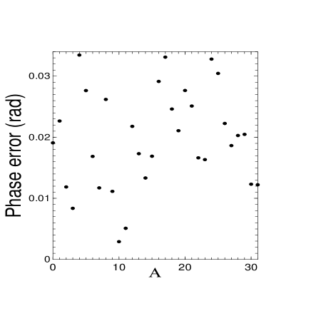
Figure 1: Phase error after implementation of the full adder for different values of the addend number A. $K=8$ [$\Omega\approx J/8$, see Eq. (3)], $\delta\omega/\Omega=10^{4}$ ($\delta\omega\approx 1252J$), $l=5$ ($L=11$).

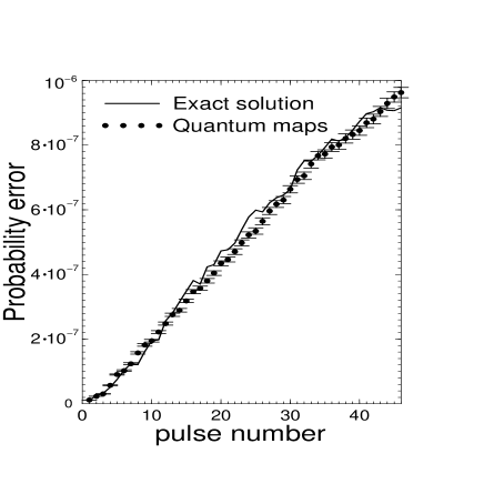
Figure 2: The probability error as a function of the number of Q-pulses during implementation of the full adder obtained using exact solution and using quantum maps. $K=100$ ($\Omega\approx 0.01$), $\delta\omega=100$, $l=4$ ($L=9$). The data obtained using the quantum maps are averaged over 100 realization with different sets of the random phases.

VI.2 Test of the quantum map approach

Since we used random phases for probability amplitudes generated by the unwanted transitions instead of their actual phases, we tested our approach by comparison with the exact numerical solution. In Fig. 2 we compare the probability errors calculated using quantum maps with the probability errors computed using the exact solution for $L=9$ qubits. The initial superposition contained the numbers 2, 5, 11, 12 with randomly chosen normalized coefficients $C_{B_{i}}(0)$ and A=6. The probability error for the exact case is defined as

$$P=\sum_{i=1}^{M}||C_{G_{i}}(T)|^{2}-|C_{B_{i}}(0)|^{2}|,$$ (23)

while the probability error using quantum maps is defined as the sum of the probabilities of all unwanted states. As follows from Fig. 2, there is good correspondence between the data obtained using the exact numerical solution and the results obtained using the quantum maps. We observed a similar correspondence for the other initial conditions and other addend numbers A.

Figure 3: The probability error as a function of the number of Q-pulses during implementation of the full adder obtained using quantum maps. $K=100$ ($\Omega\approx 0.01$), $\delta\omega=100$. Number of addend qubits is $l=1000$ and the total number of qubits is $L=2001$.

VI.3 Modeling the full adder with 1000 addend qubits

The growth of error with increasing the number of pulses is shown in Fig. 3. This figure is obtained using quantum maps with 20 randomly chosen initial numbers, $B_{i}$, with randomly chosen normalized coefficients, $C_{B_{i}}(0)$. The data are averaged over 20 different realizations with different sets of the random phases. The error bars are of the order of or less than the line width. We also modeled the full adder for superposition of 1 and 100 states and obtained the same curve as in Fig. 3, so that the probability error appears to be independent of the number of states in the superposition. During modeling only the unwanted states with probabilities $\xi\geq 0.001(\Omega/\delta\omega)^{2}/M$ were taken into consideration. All other unwanted states with the smaller probabilities were neglected. Decreasing the value of $\xi$ did not significantly affect the value of the probability error. As discussed above, the probability error in Fig. 3 grows linearly and is approximately equal to $N(\Omega/\delta\omega)^{2}$, where $N$ is the number of pulses. In Fig. 4 we plot the number of unwanted states generated by one useful state as a function of the number of Q-pulses. If the initial superposition contains $M$ useful states the number of unwanted states must be multiplied by $M$.

Figure 4: The growth of the number of unwanted states generated by one useful state as a function of the number of Q-pulses implementing the full adder protocol. The parameters are the same as in Fig. 3. The data are averaged over 100 quantum map realizations.

VII Conclusion

We have successfully demonstrated in this paper that a very efficient mapping procedure can closely approximate exact quantum dynamics of quantum computer. Our quantum map approach can also be generalized for use in other models, including models with time-dependent Hamiltonians. (Our Hamiltonian is time-independent in the rotating frame.) For a model with nearest neighbor constant interaction between the qubits, the result of the action of a pulse depends on the frequency difference between $k$th and $k^{\prime}$th spin and on orientations of the following spins: $k$th spin with resonant or near-resonant frequency; $(k-1)$th and $(k+1)$th spins; $k^{\prime}$th spin with nonresonant frequency, whose flip creates an error; $(k^{\prime}-1)$th and $(k^{\prime}+1)$th spins. The number of these possible configurations is relatively small even for a computer with large number of qubits. Even in the case when the analytic solution is unknown, the results of the action of a single pulse on the finite number of possible spin configurations enumerated above can be calculated numerically to define the moduli for the transition amplitudes of one step of the discrete map. As shown in this paper the phases of the generated unwanted states can be assumed to be random. After identifying the maps, one can use them to simulate a whole quantum protocol.

The quantum map method is similar to dynamical simulations of quantum systems with time-periodic Hamiltonians using the Floquet theorem Reichl ; Reichl1 ; chaos . In the latter approach one calculates the dynamics for one period of external field, ${\cal T}$. Then one builds the evolution operator for one period, and then the evolution operator for one period can be used to find the state of the system at time $m{\cal T}$, $m=2,3\dots$, without integration of the Schrödinger equation for this time. The Floquet theorem is especially useful for finding the asymptotic behavior of the system, for $m\rightarrow\infty$. Similarly, the quantum map approach is most useful when a quantum protocol contains a large number of pulses and when the number of qubits in the register of a quantum computer is large.

- (1) G. P. Berman, D. I. Kamenev, R. B. Kassman, C. Pineda, V. I. Tsifrinovich, Int. J. Quant. Inf., 1, 51 (2003).
- (2) G. P. Berman, D. I. Kamenev, V. I. Tsifrinovich, Journal of Applied Mathematics, 2003:1, 35 (2003).
- (3) G. P. Berman, G. D. Doolen, G. V. Lopez, V. I. Tsifrinovich, Comp. Phys. Commun., 146, 324 (2002).
- (4) G. P. Berman, G. D. Doolen, D. I. Kamenev, V. I. Tsifrinovich, Phys. Rev. A, 65, 012321 (2002).
- (5) G. P. Berman, G. D. Doolen, D. I. Kamenev, G. V. López, V. I. Tsifrinovich, Contemporary Mathematics, 305, 13 (2002).
- (6) G. P. Berman, G. V. López, V. I. Tsifrinovich, Phys. Rev. A, 66, 042312 (2002).
- (7) G. P. Berman, F. Borgonovi, G. Celardo, F. M. Izrailev, D. I. Kamenev, Phys. Rev. E 66, 056206 (2002).
- (8) G. P. Berman, G. D. Doolen, D. I. Kamenev, V. I. Tsifrinovich, in Proceedings of the 1st International Conference on Experimental Implementation of Quantum Computation, Sydney, Australia, 2001, Ed.: R.G. Clark, p. 160 (2001).
- (9) G. P. Berman, D. I. Kamenev, V. I. Tsifrinovich, quant-ph/0310049 (2003).
- (10) G. P. Berman, G. D. Doolen, G. V. Lòpez, V. I. Tsifrinovich, Phys. Rev. A 61, 062305 (2000).
- (11) M. Drndić, K. S. Johnson, J. H. Thywissen, M. Prentiss, R. M. Westervelt, Appl. Phys. Lett. 72, 2906 (1998).
- (12) D. Suter, K. Lim, Phys. Rev. A 65, 052309 (2002).
- (13) J. R. Goldman, T. D. Ladd, F. Yamaguchi, Y. Yamamoto, Appl. Phys. A 71, 11 (2000).
- (14) D. Beckman, A. N. Chari, S. Devabhaktuni, J. Preskill, Phys. Rev. A 54, 1034 (1996).
- (15) G. P. Berman, G. D. Doolen, V. I. Tsifrinovich, Phys. Rev. Lett. 84, 1615 (2000).
- (16) W. A. Lin, L. E. Reichl, Phys. Rev. A 40, 1055 (1989).
- (17) L. E. Reichl, The Transition to Chaos (Springer-Verlag, New York, 1992), p.385.
- (18) V. Ya. Demikhovskii, D. I. Kamenev, G. A. Luna-Acosta, Phys. Rev. E 59, 294 (1999).