Probability tables

Abstract

The idea of writing a table of probabilistic data for a quantum or classical system, and of decomposing this table in a compact way, leads to a shortcut for Hardy’s formalism, and gives new perspectives on foundational issues.

1 Introduction

Suppose that we have written, in a sort of table, the statistical data collected from a group of experiments — the nature of which can be classical, quantum, or something else. Suppose that we also want to store this table’s data in a compact way. How could we proceed?

In this paper it is shown that, given the situation described above, when we try to store or organise the table’s data in a more compact way we find that real vectors can be associated to preparations and results, in a way which, for quantum mechanical phenomena, is essentially the same as Hardy’s representation of ‘states’ and ‘measurement outcomes’ [1]. This curious fact may offer new points of view for looking at some of the current ‘foundational’ issues in quantum mechanics.

The ideas here presented are a summary of those developed in Ref. 2, to which the Reader is referred for further details. The emphasis in this paper is on the main idea of a ‘table decomposition’, and on the implications of the latter for various topics discussed in this Conference.

2 Probability tables

Imagine that we are in a laboratory, performing experiments of various kinds to study some interesting phenomena; the purpose of the experiments is to statistically study the correlations among different kinds of these phenomena. In general, we try to reproduce a given phenomenon — either by controllably preparing it at will, or simply by waiting for its occurrence —, to observe which concomitant phenomena, or results, occur.

Some experiments present common features: for example, part of the preparation can be the same for some of them. We separate ideally each experiment into a preparation and an intervention; the latter also delimits the kind of results which can be obtained, which implies that if we are told a result, we know which intervention was made. We then consider a set of preparations and a set of interventions, with the clause that sensible experiments may be made by combining each of the preparations with each of the interventions (preparations or interventions which do not satisfy this condition are set aside for the moment).

Thus, suppose that we have $M$ different preparations $\{\textsf{\emph{S}}_{1},\dotsc,\textsf{\emph{S}}_{M}\}$, and a given number of possible interventions $\{\textsf{\emph{M}}_{1},\textsf{\emph{M}}_{2},\dotsc,\textsf{\emph{M}}_{k},\dotsc\}$, each with a different number $I_{\textsf{\emph{M}}_{k}}$ of results $\{\textsf{\emph{R}}_{1},\textsf{\emph{R}}_{2},\dotsc,\textsf{\emph{R}}_{I_{\textsf{\emph{M}}_{k}}}\}$ (mutually exclusive and exhaustive), where the number $I_{\textsf{\emph{M}}_{k}}$ depends on the particular intervention $\textsf{\emph{M}}_{k}$. The total number of results, counted from all interventions, is $L$.

Through repetitions of the experiments, or through theoretical assumptions, or just by analogy with other experiments which we have already seen and which we judge similar to those that are now under study, we can write down a table $\bm{p}$ with the probabilities that we assign to every result, for every intervention and preparation. The table may look like the following:

		$\textsf{\emph{S}}_{1}$	$\textsf{\emph{S}}_{2}$	$\textsf{\emph{S}}_{3}$	$\textsf{\emph{S}}_{4}$	$\dotso$	$\textsf{\emph{S}}_{M}$
$\textsf{\emph{M}}_{1}$	$\textsf{\emph{R}}_{1}$ $\textsf{\emph{R}}_{2}$	$p_{11}$ $p_{21}$	$p_{12}$ $p_{22}$	$p_{13}$ $p_{23}$	$p_{14}$ $p_{24}$	$\dotso$ $\dotso$	$p_{1M}$ $p_{2M}$
$\textsf{\emph{M}}_{2}$	$\textsf{\emph{R}}_{3}$ $\textsf{\emph{R}}_{4}$ $\textsf{\emph{R}}_{5}$	$p_{31}$ $p_{41}$ $p_{51}$	$p_{32}$ $p_{42}$ $p_{52}$	$p_{33}$ $p_{43}$ $p_{53}$	$p_{34}$ $p_{44}$ $p_{54}$	$\dotso$ $\dotso$ $\dotso$	$p_{3M}$ $p_{4M}$ $p_{5M}$
$\textsf{\emph{M}}_{3}$	$\textsf{\emph{R}}_{6}$ $\dotso$ $\textsf{\emph{R}}_{L}$	$p_{61}$ $\dotso$ $p_{L1}$	$p_{62}$ $\dotso$ $p_{L2}$	$p_{63}$ $\dotso$ $p_{L3}$	$p_{64}$ $\dotso$ $p_{L4}$	$\dotso$ $\dotso$ $\dotso$	$p_{6M}$ $\dotso$ $p_{LM}$

The table, which may be called a ‘probability table’, has a column for each preparation and a group of rows for each intervention, and these rows are the possible results of the intervention. The table entry $p_{ij}$ is the probability of obtaining the result $\textsf{\emph{R}}_{i}$ for the intervention $\textsf{\emph{M}}_{k_{i}}$ and the preparation $\textsf{\emph{S}}_{j}$. For example, the entry $(4,3)$ is the probability $p_{4\,3}$ the we assign to obtaining the result $\textsf{\emph{R}}_{4}$, among the possible results $\{\textsf{\emph{R}}_{3},\textsf{\emph{R}}_{4},\textsf{\emph{R}}_{5}\}$, for the intervention $\textsf{\emph{M}}_{2}$ and the preparation $\textsf{\emph{S}}_{3}$. Preparations and results can be listed and rearranged in any desired way in the table. Such a table would very likely have a large number of rows and columns, i.e., the numbers $L$ and $M$ are likely to be very large.

Now, suppose that we seek a more compact way to write down and store the probability data collected in the table $\bm{p}$. We note that the table is really just an $L\times M$ rectangular matrix, and as such it has a rank $K$, viz., the minimum number of linearly independent rows or columns:

$$K\stackrel{{\scriptstyle\text{\tiny def}}}{{=}}\operatorname{rank}\bm{p}\leqslant\min\{L,M\}.$$ (1)

It follows from linear algebra that $\bm{p}$ can be written as the product of an $L\times K$ matrix $\bm{t}$ and a $K\times M$ matrix $\bm{u}$:

$$\bm{p}=\bm{t}\,\bm{u},$$ (2)

or

$$\left(\begin{smallmatrix}p_{11}&\dots&p_{1j}&\dots&p_{1M}\\ \dots&\dots&\dots&\dots&\dots\\ p_{i1}&\dots&p_{ij}&\dots&p_{iM}\\ \dots&\dots&\dots&\dots&\dots\\ p_{L1}&\dots&p_{Lj}&\dots&p_{LM}\end{smallmatrix}\right)=\left(\begin{smallmatrix}\bm{r}_{1}^{\mathsf{T}}\\ \dots\\ \bm{r}_{i}^{\mathsf{T}}\\ \dots\\ \bm{r}_{L}^{\mathsf{T}}\end{smallmatrix}\right)\left(\begin{smallmatrix}\bm{s}_{1}&\dots&\bm{s}_{j}&\dots&\bm{s}_{M}\\ \end{smallmatrix}\right)$$ (3)

In the last equation, the matrix $\bm{t}$ has been written as a block of row vectors $\bm{r}_{i}^{\mathsf{T}}$, and the matrix $\bm{u}$ as a block of column vectors $\bm{s}_{i}$. In this decomposition, the element $p_{ij}$ of $\bm{p}$ is then given by the matrix product of the row vector $\bm{r}_{i}^{\mathsf{T}}$ with the column vector $\bm{s}_{j}$:

$$p_{ij}=\bm{r}_{i}^{\mathsf{T}}\bm{s}_{j}=\bm{r}_{i}\cdot\bm{s}_{j},$$ (4)

where, in the last expression, $\bm{r}_{i}$ and $\bm{s}_{j}$ are considered as vectors in $\mathbb{R}^{K}$, so that the matrix product is equivalent to the scalar product. It will be shown in a moment that the decomposition is always effective in reducing the number of data of the table.

The result is that we can associate vectors $\{\bm{s}_{j}\}$ and $\{\bm{r}_{i}\}$ in $\mathbb{R}^{K}$, for some $K$, to the preparations and the intervention results for the table, and the relative probabilities are given by their scalar product:

$$p_{ij}\equiv\bm{r}_{i}\cdot\bm{s}_{j}.$$ (5)

These vectors can be called preparation vectors and (intervention-)result vectors, or, in general, (table) vectors.

It should be remarked immediately that we are not postulating any kind of physical property in Eq. (5); even less have we found one. We have only decided to represent and store a collection of numbers (which do have physical significance) in an alternative way. Note, in particular, that the numerical values of the vectors $\{\bm{s}_{j}\}$ and $\{\bm{r}_{i}\}$, as well as their dimension $K$, depend on the whole collection of probabilities $\{p_{ij}\}$: if one of these is changed, then $K$ and all the vectors will in general change.

The meaning of the representation (5) shall be discussed in a moment, but let us study the decomposition in more detail first, in order to have a clearer idea of how the table vectors originate.

The matrices $\bm{t}$ and $\bm{u}$ are not uniquely determined from the decomposition (2), so that there is some freedom in choosing their form. The fact that $\operatorname{rank}\bm{p}=K$, implies that there exists a square $K\times K$ submatrix $\bm{a}$, obtained from $\bm{p}$ by suppressing $(L-K)$ rows and $(M-K)$ columns, such that $\det\bm{a}\neq 0$. It is always possible to rearrange the rows and the columns of the table $\bm{p}$ so that this non-singular submatrix is the one formed by the first $K$ rows and $K$ columns. After this rearrangement, $\bm{p}$ can be written in the following block form:

$$\bm{p}=\begin{pmatrix}\bm{a}&\bm{b}\\ \bm{c}&\bm{d}\end{pmatrix}\quad\text{with $\det\bm{a}\neq 0$},$$ (6)

where $\bm{b}$, $\bm{c}$, and $\bm{d}$ are of order $K\times(M-K)$, $(L-K)\times K$, and $(L-K)\times(M-K)$ respectively.

By writing also the matrices $\bm{t}$ and $\bm{u}$ in block form

$$\bm{t}=\begin{pmatrix}\bm{v}\\ \bm{w}\end{pmatrix},\quad\bm{u}=\begin{pmatrix}\bm{x}&\bm{y}\end{pmatrix},$$ (7)

where the orders of $\bm{v}$, $\bm{w}$, $\bm{x}$, and $\bm{y}$ are $K\times K$, $(L-K)\times K$, $K\times K$, and $K\times(M-K)$ respectively, we can rewrite the decomposition equation (2) as

$$\begin{pmatrix}\bm{a}&\bm{b}\\ \bm{c}&\bm{d}\end{pmatrix}=\begin{pmatrix}\bm{v}\\ \bm{w}\end{pmatrix}\begin{pmatrix}\bm{x}&\bm{y}\end{pmatrix},$$ (8)

or

$$\begin{aligned} \bm{a}&=\bm{v}\bm{x},&\bm{b}&=\bm{v}\bm{y},&\bm{c}&=\bm{w}\bm{x},&\bm{d}&=\bm{w}\bm{y},\end{aligned}$$ (9)

which has the solution

$$\det\bm{x} \neq 0, \bm{y} =\bm{x}\bm{a}^{-1}\bm{b}, \bm{v} =\bm{a}\bm{x}^{-1}, \bm{w} =\bm{c}\bm{x}^{-1},$$ (10)

which in terms of the result and preparation vectors is

$$\begin{aligned} (\bm{s}_{1}\;\dots\;\bm{s}_{K})&=\bm{x},&(\bm{s}_{K+1}\;\dots\;\bm{s}_{M})&=\bm{x}\bm{a}^{-1}\bm{b},\end{aligned}$$ (11a)

$$\begin{aligned} \begin{pmatrix}\bm{r}_{1}\\ \dots\\ \bm{r}_{K}\end{pmatrix}&=\bm{a}\bm{x}^{-1},&\begin{pmatrix}\bm{r}_{K+1}\\ \dots\\ \bm{r}_{L}\end{pmatrix}&=\bm{c}\bm{x}^{-1}.\end{aligned}$$ (11b)

The square matrix $\bm{x}=(\bm{s}_{1}\;\dots\;\bm{s}_{K})$ is undetermined except for the condition of being non-singular; this corresponds to the freedom of choosing $K$ basis vectors in $\mathbb{R}^{K}$ as those associated to the first $K$ preparations $\textsf{\emph{S}}_{1},\dotsc,\textsf{\emph{S}}_{K}$, which can then be called basis preparation-vectors. Note that for a given probability table $\bm{p}$ the set of basis preparation-vectors is in general non-unique, because $\bm{p}$ possesses in general many submatrices like $\bm{a}$ with rank $K$.

We can now check whether the above decomposition effectively reduces the number of data to be stored. The table $\bm{p}$ has $L\times M$ entries. The matrices $\bm{x}$, $\bm{y}$, $\bm{v}$, $\bm{w}$ (or equivalently the collection of vectors $\{\bm{s}_{j}\}$ and $\{\bm{r}_{i}\}$) have in total $K\times(L+M)$ entries; however, we are free to choose a ‘canonical’ form for the non-singular $K\times K$ matrix $\bm{x}$ (e.g., the identity matrix) once and for all, for all probability tables (this corresponds to a standard choice of basis vectors in $\mathbb{R}^{K}$). This implies that we are indeed left with only $K\times(L+M)-K^{2}$ numbers. It is then simple to verify that, from $K\leqslant\min\{L,M\}$, we have

$$K\times(L+M)-K^{2}\leqslant L\times M.$$ (12)

Thus the decomposition of the probability table into two sets of vectors is indeed a more compact way to write down and store the probability data.

2.1 A numerical and graphical example

Imagine that, with the various apparatus in our laboratory, we can make seven different preparations $\{\textsf{\emph{S}}_{1},\dotsc,\textsf{\emph{S}}_{7}\}$ and perform three different interventions $\{\textsf{\emph{M}}_{1},\textsf{\emph{M}}_{2},\textsf{\emph{M}}_{3}\}$, each having two results. The probabilities that we assign to the various results are given in the following table:

		$\textsf{\emph{S}}_{1}$	$\textsf{\emph{S}}_{2}$	$\textsf{\emph{S}}_{3}$	$\textsf{\emph{S}}_{4}$	$\textsf{\emph{S}}_{5}$	$\textsf{\emph{S}}_{6}$	$\textsf{\emph{S}}_{7}$
$\textsf{\emph{M}}_{1}$	$\textsf{\emph{R}}_{1}$ $\textsf{\emph{R}}_{2}$	1 0	$\tfrac{1}{2}$ $\tfrac{1}{2}$	0 1	$\tfrac{1}{2}$ $\tfrac{1}{2}$	$\tfrac{3}{4}$ $\tfrac{1}{4}$	$\tfrac{1}{2}$ $\tfrac{1}{2}$	$\tfrac{3}{4}$ $\tfrac{1}{4}$
$\textsf{\emph{M}}_{2}$	$\textsf{\emph{R}}_{3}$ $\textsf{\emph{R}}_{4}$	$\tfrac{1}{2}$ $\tfrac{1}{2}$	1 0	$\tfrac{1}{2}$ $\tfrac{1}{2}$	0 1	$\tfrac{3}{4}$ $\tfrac{1}{4}$	$\tfrac{1}{2}$ $\tfrac{1}{2}$	$\tfrac{1}{2}$ $\tfrac{1}{2}$
$\textsf{\emph{M}}_{3}$	$\textsf{\emph{R}}_{5}$ $\textsf{\emph{R}}_{6}$	1 0	1 0	1 0	1 0	1 0	1 0	1 0

The matrix corresponding to this probability table has rank $K=3$, and the first $3\times 3$ submatrix $\bm{a}$ is indeed already non-singular, without the need of rearranging the rows or columns of the original table. Proceeding as in the decomposition equations (9) and (10) with the following choice for the matrix $\bm{x}$:

$$\bm{x}\equiv\begin{pmatrix}1&1&1\\ 1&0&-1\\ 0&1&0\end{pmatrix},$$ (13)

we finally obtain the following preparation and result vectors:

$$\begin{aligned} \bm{s}_{1}&=(1,1,0),\\ \bm{s}_{2}&=(1,0,1),\\ \bm{s}_{3}&=(1,-1,0),\\ \bm{s}_{4}&=(1,0,-1),\\ \bm{s}_{5}&=(1,\tfrac{1}{2},\tfrac{1}{2}),\\ \bm{s}_{6}&=(1,0,0),\\ \bm{s}_{7}&=(1,\tfrac{1}{2},0),\end{aligned} \begin{aligned} \bm{r}_{1}&=(\tfrac{1}{2},\tfrac{1}{2},0),\\ \bm{r}_{2}&=(\tfrac{1}{2},-\tfrac{1}{2},0),\\ \bm{r}_{3}&=(\tfrac{1}{2},0,\tfrac{1}{2}),\\ \bm{r}_{4}&=(\tfrac{1}{2},0,-\tfrac{1}{2}),\\ \bm{r}_{5}&=(1,0,0),\\ \bm{r}_{6}&=\bm{O}=(0,0,0),\\ \end{aligned}$$ (14)

represented as points of $\mathbb{R}^{3}$ in Fig. 1.

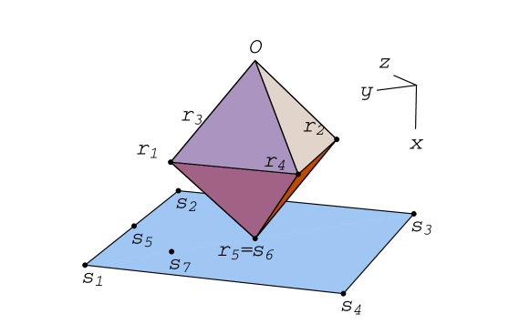
Figure 1: Preparation and result vectors (and their convex hulls) in $\mathbb{R}^{3}$, from the example. $O$ is the origin; $x$, $y$, $z$ are the directions of the Cartesian axes.

We notice that all preparation vectors lie on the same plane ($x=1$); this is a general property of any probability table, which derives from the fact that the results of an intervention are mutually exclusive and exhaustive; this also implies that an intervention’s result-vectors always sum up to the same vector [2]: in this case, $\bm{r}_{1}+\bm{r}_{2}=\bm{r}_{3}+\bm{r}_{4}=\bm{r}_{5}+\bm{r}_{6}=(1,0,0)$.

3 Relation to quantum mechanics

Probability tables like the one illustrated above can be made, in particular, for phenomena concerning classical or quantum systems. Indeed, the resulting association of vectors to preparations and results is analogous to that introduced by Hardy [1], through a different line of reasoning, for ‘states’ and ‘measurement outcomes’ of classical and quantum systems.

For example, imagine how a table for a two-level quantum system would appear; consider for concreteness the polarisation of a single photon. We can prepare the photon with different polarisation directions and with different degrees of polarisation; hence the table has in the limit a continuum of columns, one for each preparation. Analogously, we can perform some interventions on the photon by placing various polarisation filters on its way, controlling if it is absorbed or not; in the limit, the table has also a continuum of rows, one for each intervention result. Some entries of the table would look like the following (the meaning of the symbols should be self-evident):

		$\dots$	$\textsf{\emph{S}}_{0^{\mathord{\circ}}}$	$\dots$	$\textsf{\emph{S}}_{45^{\mathord{\circ}}}$	$\dots$
$\dots$	$\dots$	$\dots$	$\dots$	$\dots$	$\dots$	$\dots$
$\textsf{\emph{M}}_{45^{\mathord{\circ}}}$	$\textsf{\emph{R}}_{\text{out}}^{45^{\mathord{\circ}}}$ $\textsf{\emph{R}}_{\text{abs}}^{45^{\mathord{\circ}}}$	$\dotso$ $\dotso$	$\tfrac{1}{2}$ $\tfrac{1}{2}$	$\dotso$ $\dotso$	1 0	$\dotso$ $\dotso$
$\dots$	$\dots$	$\dots$	$\dots$	$\dots$	$\dots$	$\dots$
$\textsf{\emph{M}}_{60^{\mathord{\circ}}}$	$\textsf{\emph{R}}_{\text{out}}^{60^{\mathord{\circ}}}$ $\textsf{\emph{R}}_{\text{abs}}^{60^{\mathord{\circ}}}$	$\dotso$ $\dotso$	$\tfrac{1}{4}$ $\tfrac{3}{4}$	$\dotso$ $\dotso$	$0.933$ $0.067$	$\dotso$ $\dotso$
$\dots$	$\dots$	$\dots$	$\dots$	$\dots$	$\dots$	$\dots$

Such a table has, notwithstanding the limiting infinite size, rank $K=4$, and so we can associate to every preparation and to every result a $4$-dimensional vector. The preparation vectors, however, lie on a $3$-dimensional (affine) hyper-plane, as in the numerical example previously discussed. It can be shown indeed [1, 2] that the resulting set of preparation vectors is equivalent to the standard Bloch-sphere for two-level quantum systems.

This was just an example, but all quantum-mechanical concepts like density matrix, positive-operator-valued measure, and completely positive map can be expressed in an equivalent table-vector formalism [1, 2] (e.g., the relation with the trace rule is quickly shown in the appendix).

4 Discussion

The following discussion concentrates on the possible relations among the ideas hitherto presented and ideas presented by other authors in this Conference. The Reader is referred to Ref. 2 for a more general and detailed discussion.

4.1 On the probabilities in the table and ‘quantum logics’

In Sect. 2, we quickly introduced the preparations, interventions, and results $\{\textsf{\emph{S}}_{j}\}$, $\{\textsf{\emph{M}}_{k}\}$, $\{\textsf{\emph{R}}_{i}\}$, and the probabilities $\{p_{ij}\}$ which make up the table. Let us define them more clearly.

Symbols like $\textsf{\emph{S}}_{i}$ and $\textsf{\emph{M}}_{k}$ represent propositions which together describe an actual, well-defined procedure to set up an experiment, e.g. $\textsf{\emph{S}}_{i}=$‘The diode laser is put on the table is such and such position, with a beam splitter in front of it in such and such position…’ etc., and $\textsf{\emph{M}}_{k}=$‘Such and such vertical filter is placed in such and such place, and the detector is placed behind it…’ etc. The separation of the experiment’s description into the two propositions is not unique, and indeed more kinds of separations can be considered.

A symbol like $\textsf{\emph{R}}_{j}$ represents a proposition which describes the results of an experiment, e.g. $\textsf{\emph{R}}_{j}=$‘The detector does not click’; it is then clear that it depends on the particular experiment being performed.

The probability $p_{ij}$ is consequently defined as

$$p_{ij}\stackrel{{\scriptstyle\text{\tiny def}}}{{=}}P(\textsf{\emph{R}}_{i}\mathpunct{|}\textsf{\emph{M}}_{k_{i}}\land\textsf{\emph{S}}_{j}\land\textsf{\emph{Q}}),$$ (15)

where Q is a proposition representing the rest of the experimental details and our prior knowledge. We are thus considering probability theory as extended logic [13, 14, 15, 16], an approach which will prove to be, in the following, powerful, flexible, and intuitive at once.

Usually, many repetitions of the same experiment are made and the relative frequencies of the different results of the intervention are observed. In this case, given a judgement of total exchangeability of the experiment’s repetitions, the probability is practically equal to the observed frequency of the result, thanks to de Finetti’s representation theorem [17]. But the probability can also be assigned on grounds of similarity with other experiments, or just by theoretical assumptions.

Note that the table is silent with regard to the probabilities for the preparations or the interventions, $P(\textsf{\emph{S}}_{j}\mathpunct{|}\textsf{\emph{Q}})$ and $P(\textsf{\emph{M}}_{k}\mathpunct{|}\textsf{\emph{Q}})$. In a given ‘situation’ Q, if we decide which preparation and intervention to perform, say $\textsf{\emph{S}}_{5}$ and $\textsf{\emph{M}}_{7}$, then these probabilities are $P(\textsf{\emph{S}}_{i}\mathpunct{|}\textsf{\emph{Q}})={}_{i,5}$ and $P(\textsf{\emph{M}}_{k}\mathpunct{|}\textsf{\emph{Q}})={}_{k,7}$ of course (which amounts to saying that “we know what we’re doing”). If it is someone else who is deciding the particular preparation and intervention, then the probabilities must be assigned in some other way, e.g. by asking “which preparation are you making?”, or by using some other knowledge, and they will in general differ from $0$ and $1$. The difference between these probabilities and those of Eq. (15) is somehow analogous to the difference between initial conditions and equations of motion in classical mechanics: the theory concerns only the latter, while the former has to be specified on a case-by-case basis.

The probabilities of the results of a given intervention and a given preparation form a probability distribution, because the results were arranged so as to be mutually exclusive and exhaustive. This implies that, for two results $\textsf{\emph{R}}_{k}$ and $\textsf{\emph{R}}_{k}^{\prime}$ of a given intervention $\textsf{\emph{M}}_{k}$ and for a given preparation $\textsf{\emph{S}}_{j}$, we also have the trivial identity

$$\begin{split}P(\textsf{\emph{R}}_{k}\lor\textsf{\emph{R}}_{k}^{\prime}\mathpunct{|}\textsf{\emph{M}}_{k}\land\textsf{\emph{S}}_{j}\land\textsf{\emph{Q}})&=P(\textsf{\emph{R}}_{k}\mathpunct{|}\textsf{\emph{M}}_{k}\land\textsf{\emph{S}}_{j}\land\textsf{\emph{Q}})+P(\textsf{\emph{R}}_{k}^{\prime}\mathpunct{|}\textsf{\emph{M}}_{k}\land\textsf{\emph{S}}_{j}\land\textsf{\emph{Q}}),\\ &=(\bm{r}_{k}+\bm{r}_{k}^{\prime})\cdot\bm{s}_{j}.\end{split}$$ (16)

But with probability theory as logic we can also evaluate, for a given preparation $\textsf{\emph{S}}_{j}$, the disjoint probability for the results $\textsf{\emph{R}}^{\prime}$ and $\textsf{\emph{R}}^{\prime\prime}$ of two different interventions $\textsf{\emph{M}}^{\prime}$ and $\textsf{\emph{M}}^{\prime\prime}$, just using the product and sum rules:

$$\begin{split}P[\textsf{\emph{R}}^{\prime}\lor\textsf{\emph{R}}^{\prime\prime}\mathpunct{|}(\textsf{\emph{M}}^{\prime}\lor\textsf{\emph{M}}^{\prime\prime})\land\textsf{\emph{S}}_{j}\land\textsf{\emph{Q}}]&=P[(\textsf{\emph{R}}^{\prime}\land\textsf{\emph{M}}^{\prime})\lor(\textsf{\emph{R}}^{\prime\prime}\land\textsf{\emph{M}}^{\prime\prime})\mathpunct{|}\textsf{\emph{S}}_{j}\land\textsf{\emph{Q}}],\\ &=\begin{aligned} &P(\textsf{\emph{R}}^{\prime}\mathpunct{|}\textsf{\emph{M}}^{\prime}\land\textsf{\emph{S}}_{j}\land\textsf{\emph{Q}})\times P(\textsf{\emph{M}}^{\prime}\mathpunct{|}\textsf{\emph{S}}_{j}\land\textsf{\emph{Q}})+\mbox{}\\ &P(\textsf{\emph{R}}^{\prime\prime}\mathpunct{|}\textsf{\emph{M}}^{\prime\prime}\land\textsf{\emph{S}}_{j}\land\textsf{\emph{Q}})\times P(\textsf{\emph{M}}^{\prime\prime}\mathpunct{|}\textsf{\emph{S}}_{j}\land\textsf{\emph{Q}}),\end{aligned}\\ &=[\bm{r}^{\prime}P(\textsf{\emph{M}}^{\prime}\mathpunct{|}\textsf{\emph{S}}_{j}\land\textsf{\emph{Q}})+\bm{r}^{\prime\prime}P(\textsf{\emph{M}}^{\prime\prime}\mathpunct{|}\textsf{\emph{S}}_{j}\land\textsf{\emph{Q}})]\cdot\bm{s}_{j},\end{split}$$ (17)

where it is assumed that $P(\textsf{\emph{M}}^{\prime}\lor\textsf{\emph{M}}^{\prime\prime}\mathpunct{|}\textsf{\emph{S}}_{j}\land\textsf{\emph{Q}})=1$, i.e., we are sure that one or the other intervention was performed.

The content of the formula above is intuitive: the occurrence of the result $\textsf{\emph{R}}^{\prime}$ implies that the intervention $\textsf{\emph{M}}^{\prime}$ was performed, and so analogously for the result $\textsf{\emph{R}}^{\prime\prime}$ and the intervention $\textsf{\emph{M}}^{\prime\prime}$. Then the probability of getting the one or the other result depends in turn on the probability that the one or the other intervention was made, hence these probabilities appear in the last line of the above equation. However, as already said, the probabilities of these interventions are not contained in the table, but must be given on a case-by-case basis.

As a result, the two disjoint probabilities in Eqs. (16) and (17) ‘behave’ differently, and the reason for this is intuitively clear. However, we can partially trace in this fact the source of much research and discussion on partially ordered lattices and quantum logics for the set of intervention results [18, 19, 20]. Roughly speaking, the point is that, for a classical system, there is the theoretical possibility of joining all possible interventions (measurements) in a single “total intervention”: the table associated to a classical system can then be considered as having only one intervention; thus one needs never consider the case of Eq. (17). However, such “total intervention” is excluded in quantum mechanics, and one is thus forced to consider the case of Eq. (17).

From the point of view of probability theory as logic, instead, there is no need for non-Boolean structures thanks to the possibility of changing and adapting, by means of Bayes’ theorem, the context (also called ‘prior knowledge’ [16] or ‘data’ [13]) of a probability, i.e., the proposition to the right of the conditional symbol ‘$\mathpunct{|}$’.

4.2 Unknown preparations and their ‘tomography’

On the other hand, we may have the following scenario: we have repeated instances of a given preparation, but we do not know which. By performing interventions on these instances and observing the results, we can estimate which preparation is being made. Introducing the proposition $D$ representing the results thus obtained, we have

$$P(\textsf{\emph{S}}_{j}\mathpunct{|}D\land\textsf{\emph{Q}})=\frac{P(D\mathpunct{|}\textsf{\emph{S}}_{j}\land\textsf{\emph{Q}})\,P(\textsf{\emph{S}}_{j}\mathpunct{|}\textsf{\emph{Q}})}{\sum_{j}P(D\mathpunct{|}\textsf{\emph{S}}_{j}\land\textsf{\emph{Q}})\,P(\textsf{\emph{S}}_{j}\mathpunct{|}\textsf{\emph{Q}})}.$$ (18)

This is a standard “inverse-inference” result of Bayesian analysis [16, Ch. 4]. The probability $P(D\mathpunct{|}\textsf{\emph{S}}_{j}\land\textsf{\emph{Q}})$ can be written in terms of scalar products of result and preparation vectors, but the probability distribution $\{P(\textsf{\emph{S}}_{j}\mathpunct{|}\textsf{\emph{Q}})\}$ depends on the prior knowledge that one has in each specific case. If we now want to predict which result will occur in a new intervention $\textsf{\emph{M}}_{k}$, we have the following probability:

$$\begin{split}P(\textsf{\emph{R}}_{i}\mathpunct{|}\textsf{\emph{M}}_{k_{i}}\land D\land\textsf{\emph{Q}})&=\sum_{j}P(\textsf{\emph{R}}_{i}\mathpunct{|}\textsf{\emph{M}}_{k_{i}}\land\textsf{\emph{S}}_{j}\land\textsf{\emph{Q}})\times P(\textsf{\emph{S}}_{j}\mathpunct{|}D\land\textsf{\emph{Q}}),\\ &=\bm{r}_{i}\cdot\sum_{j}\bm{s}_{j}\>P(\textsf{\emph{S}}_{j}\mathpunct{|}D\land\textsf{\emph{Q}}),\end{split}$$ (19)

i.e., we can effectively associate the vector

$$\bm{s}_{\text{new}}\equiv\sum_{j}\bm{s}_{j}\,P(\textsf{\emph{S}}_{j}\mathpunct{|}D\land\textsf{\emph{Q}})$$ (20)

to the unknown preparation.

A further kind of scenario is this: we have a brand-new kind of preparation, i.e., a new phenomenon, still untested. It has no place in our probability table; yet we think that we could reserve a new column to it without making substantial changes to our table’s decomposition (by which we mean that the table’s rank $K$ would not change). Given this, in order to associate a vector to this new preparation we proceed as in the preceding scenario, performing interventions and observing results. The result is that Eqs. (18) and (20) also apply in this case.

Note that there is no conflict between our talking about “unknown preparations” and Fuchs’ criticism of the term ‘unknown quantum state’ [23, 24, 25]. A preparation, as we have seen, is a well-defined procedure (that can be shown or described to others, etc.) to set up a given physical situation; on the other hand, Fuchs’ meaning of ‘quantum state’ is ‘density matrix’ [23, 26], which corresponds (more or less) to the preparation vector instead. Thus, consider the two sentences “It is unknown to me which kind of laser and of beam splitter are used in this experiment” and “I do not know with which probability the detector behind the vertical filter will click”: the latter sentence is nonsensical from a Bayesian point of view, because there are no ‘unknown’ degrees of belief; but the former sentence is unquestionably meaningful. Thus, even if the preparation is unknown to us, we can always associate a preparation vector to it.

4.3 On the content of the table vectors and ‘quantum states of knowledge’

Some remarks have already been made in Sect. 2 after the derivation of the formula

$$P(\textsf{\emph{R}}_{i}\mathpunct{|}\textsf{\emph{M}}_{k_{i}}\land\textsf{\emph{S}}_{j}\land\textsf{\emph{Q}})\equiv\bm{r}_{i}\cdot\bm{s}_{j}, {}_{\text{bis}}$$ (5)

with regard to the fact that the vectors $\{\bm{s}_{j}\}$ and $\{\bm{r}_{i}\}$ do not have any physical meaning separately: a given preparation vector $\bm{s}_{j}$ tells us nothing if we do not have an intervention-result vector ${\bm{r}_{i}}$; even less if we know nothing about the set of intervention results. It follows that the preparation vectors also lack any probabilistic meaning per se: they are not probabilities nor collections of probabilities — they are just mathematical objects which yield probabilities when combined in a given way with objects of similar kind. This, in particular, is true for density matrices, as we have seen that they are just a particular case of preparation vectors. It is slightly incorrect, as well, to say that probabilities are ‘encoded’ or ‘contained’ in the (quantum) preparation vectors: rather, they are parts of an encoding.

From these considerations, the quantum state (the density matrix) appears to be part of a state of belief, and not the ‘whole’ state of belief [28, 23]. Perhaps the point is that Caves, Fuchs, and Schack’s notion of a ‘quantum’ state of belief implicitly assumes the existence and the particular structure of the whole set of quantum positive-operator-valued measures (i.e., the interventions). This is an important difference from a ‘usual’ degree of belief $P(\textsf{\emph{A}}\mathpunct{|}\textsf{\emph{X}})$ which does not need to be combined with other mathematical objects to reveal its content.

4.4 Possible applications of the table formalism

It has already been remarked that the kind of vector representation arising from the table decomposition is essentially the same as Hardy’s [1]. The derivation presented here can be seen as a sort of shortcut for his derivation, but it implies something more. Hardy supposes that it is possible to represent a preparation by means of a $K$-dimensional vector with $K\leqslant L$ because most physical theories have some structure which relates different measured quantities; but the reasoning behind the decomposition of Sect. 2 shows that this possibility exists even without a theory that describes the data (indeed, the question arises: has this possibility any physical meaning at all?)

In any case, the idea of a ‘probability table’ and its decomposition has probably very little usefulness in experimental applications, but provides a very simple approach to study the mathematical and geometrical structures of classical and quantum theories, and offers a different way to look at their “foundational” and “interpretative” issues.

This approach is even more general than other standard ones based, e.g., on $C^{*}$-algebras, or even Jordan-Banach-algebras [31], or on convex state-spaces. Thus, with the idea of a ‘probability table’ we can very easily implement ‘toy theories’ or models like those of Spekkens [32] and Kirkpatrick [33] (cf. also the issue raised by Terno [34]), which can then be compared to classical or quantum mechanics using a unique, common formalism.

Appendix A The trace rule

It is shown that the ‘scalar product formula’, Eq. (5), includes also the ‘trace rule’ of quantum mechanics (see also Ref. 1, Sect. 5).

A preparation is usually associated in quantum mechanics to a density matrix $\hat{\bm{\rho}}_{j}$, and a intervention result to a positive-operator-valued-measure element $\hat{\bm{\varPi}}_{i}$; both are Hermitian operators in a Hilbert space of dimension $N$. The probability of obtaining the result $\hat{\bm{\varPi}}_{i}$ for a given intervention on preparation $\hat{\bm{\rho}}_{j}$ is given by the trace formula

$$p_{ij}=\operatorname{tr}\hat{\bm{\varPi}}_{i}\hat{\bm{\rho}}_{j}.$$ (21)

The Hermitian operators form a linear space of real dimension $K=N^{2}$; one can choose $K$ linearly independent Hermitian operators $\{\hat{\bm{B}}_{k}\}$ as a basis for this linear space. These can also be chosen (basically by Gram-Schmidt orthonormalisation) to satisfy

$$\operatorname{tr}{\hat{\bm{B}}_{k}\hat{\bm{B}}_{l}}={}_{kl}.$$ (22)

Both $\hat{\bm{\rho}}_{j}$ and $\hat{\bm{\varPi}}_{i}$ can be written as a linear combination of the basis operators:

$$\hat{\bm{\rho}}_{j} =\sum_{l=1}^{K}{s_{j}}^{l}\hat{\bm{B}}_{l}, \hat{\bm{\varPi}}_{i} =\sum_{k=1}^{K}{r_{i}}^{k}\hat{\bm{B}}_{k},$$ (23)

where the coefficients ${s_{j}}^{l}$ and ${r_{i}}^{k}$ are real. Using Eqs. (23) and (22) the trace formula becomes

$$p_{ij}=\operatorname{tr}\hat{\bm{\varPi}}_{i}\hat{\bm{\rho}}_{j}=\sum_{k,l=1}^{K}{r_{i}}^{k}{s_{j}}^{l}\operatorname{tr}\hat{\bm{B}}_{k}\hat{\bm{B}}_{l}=\sum_{l=1}^{K}{r_{i}}^{l}{s_{j}}^{l}=\bm{r}_{i}\cdot\bm{s}_{j},$$ (24)

where $\bm{r}_{i}\stackrel{{\scriptstyle\text{\tiny def}}}{{=}}({r_{i}}^{1},\dotsc,{r_{i}}^{K})$ and $\bm{s}_{j}\stackrel{{\scriptstyle\text{\tiny def}}}{{=}}({s_{j}}^{1},\dotsc,{s_{j}}^{K})$ are vectors in $\mathbb{R}^{K}$, q.e.d.

References

- Hardy [2001] L. Hardy, Quantum theory from five reasonable axioms (2001), quant-ph/0101012.
- [2] P. G. L. Mana, in preparation.
- Mielnik [1969] B. Mielnik, Theory of filters, Commun. Math. Phys. 15, 1 (1969).
- Mielnik [1976] B. Mielnik, Quantum logic: Is it necessarily orthocomplemented?, in Quantum Mechanics, Determinism, Causality, and Particles, edited by M. Flato, Z. Maric, A. Milojevic, D. Sternheimer, and J. P. Vigier (D. Reidel Publishing Company, Dordrecht, 1976), p. 117.
- Mielnik [1981] B. Mielnik, Quantum theory without axioms, in Quantum Gravity 2, edited by C. J. Isham, R. Penrose, and D. W. Sciama (Oxford University Press, Oxford, 1981), pp. 638–656.
- Mielnik [1974] B. Mielnik, Generalized quantum mechanics, Commun. Math. Phys. 37, 221 (1974), reprinted in [35, pp. 115–152].
- Foulis and Randall [1972] D. J. Foulis and C. H. Randall, Operational statistics. I. Basic concepts, J. Math. Phys. 13, 1667 (1972).
- Randall and Foulis [1973] C. H. Randall and D. J. Foulis, Operational statistics. II. Manuals of operations and their logics, J. Math. Phys. 14, 1472 (1973).
- Foulis and Randall [1978] D. J. Foulis and C. H. Randall, Manuals, morphisms and quantum mechanics, in Mathematical Foundations of Quantum Theory, edited by A. R. Marlow (Academic Press, London, 1978), pp. 105–126.
- Randall and Foulis [1979] C. H. Randall and D. J. Foulis, The operational approach to quantum mechanics, in [35], pp. 167–201.
- Foulis and Gudder [2001] D. J. Foulis and S. P. Gudder, Observables, calibration, and effect algebras, Found. Phys. 31, 1515 (2001).
- Barnum [2003] H. Barnum, Quantum information processing, operational quantum logic, convexity, and the foundations of physics, Tech. Rep. LA-UR 03-1199, Los Alamos National Laboratory (2003), quant-ph/0304159.
- Jeffreys [1998] H. Jeffreys, Theory of Probability (Oxford University Press, London, 1998), 3rd ed., first publ. 1939.
- Cox [1946] R. T. Cox, Probability, frequency, and reasonable expectation, Am. J. Phys. 14, 1 (1946).
- Cox [1961] R. T. Cox, The Algebra of Probable Inference (The Johns Hopkins Press, Baltimore, 1961).
- Jaynes [2003] E. T. Jaynes, Probability Theory: The Logic of Science (Cambridge University Press, Cambridge, 2003), edited by G. Larry Bretthorst.
- de Finetti [1964] B. de Finetti, Foresight: Its logical laws, its subjective sources, in Studies in Subjective Probability, edited by H. E. Kyburg, Jr. and H. E. Smokler (John Wiley & Sons, New York, 1964), pp. 93–158.
- Jauch [1973] J. M. Jauch, Foundations of Quantum Mechanics (Addison-Wesley Publishing Company, Reading, USA, 1973), first publ. 1968.
- Piron [1976] C. Piron, Foundations of Quantum Physics (W. A. Benjamin, Reading, USA, 1976).
- [20] A. Wilce, Compactness and symmetry in quantum logic, in Quantum Theory: Reconsideration of Foundations. 2, to appear.
- Loubenets [2003a] E. R. Loubenets, General probabilistic framework of randomness (2003a), quant-ph/0305126.
- Loubenets [2003b] E. R. Loubenets, General framework for the probabilistic description of experiments (2003b), quant-ph/0312199.
- Fuchs [2002] C. A. Fuchs, Quantum mechanics as quantum information (and only a little more) (2002), quant-ph/0205039.
- van Enk and Fuchs [2002a] S. J. van Enk and C. A. Fuchs, Quantum state of an ideal propagating laser field, Phys. Rev. Lett. 88, 027902 (2002a), quant-ph/0104036.
- van Enk and Fuchs [2002b] S. J. van Enk and C. A. Fuchs, Quantum state of a propagating laser field, Quant. Info. Comp. 2, 151 (2002b), quant-ph/0111157.
- [26] C. A. Fuchs, Quantum states: What the Hell Are They?, http://netlib.bell-labs.com/who/cafuchs/PhaseTransition.%****␣ptables2bis.tex␣Line␣1625␣****pdf.
- Schack et al. [2001] R. Schack, T. A. Brun, and C. M. Caves, Quantum Bayes rule, Phys. Rev. A 64, 014305 (2001), quant-ph/0008113.
- Caves et al. [2002a] C. M. Caves, C. A. Fuchs, and R. Schack, Quantum probabilities as Bayesian probabilities, Phys. Rev. A 65, 022305 (2002a), quant-ph/0106133.
- Caves et al. [2002b] C. M. Caves, C. A. Fuchs, and R. Schack, Unknown quantum states: the quantum de Finetti representation, J. Math. Phys. 43, 4537 (2002b), quant-ph/0104088.
- [30] R. Schack, Unknown quantum operations, in Quantum Theory: Reconsideration of Foundations. 2, to appear.
- Halvorson [2003] H. Halvorson, A note on information theoretic characterizations of physical theories (2003), quant-ph/0310101.
- Spekkens [2004] R. W. Spekkens, In defense of the epistemic view of quantum states: a toy theory (2004), quant-ph/0401052.
- Kirkpatrick [2003] K. A. Kirkpatrick, “Quantal” behavior in classical probability, Found. Phys. Lett. 16, 199 (2003), quant-ph/0106072.
- Terno [2004] D. R. Terno, Inconsistency of quantum-classical dynamics, and what it implies (2004), quant-ph/0402092.
- Hooker [1979] C. A. Hooker, ed., Physical Theory as Logico-Operational Structure (D. Reidel Publishing Company, Dordrecht, 1979).