Contradictions of quantum scattering theory

Abstract

The standard scattering theory (SST) in non relativistic quantum mechanics is analyzed. Contradictions of SST are revealed. Justification of SST in textbooks with the help of fundamental scattering theory (FST) is shown to be unconvincing. A theory of wave packets scattering on a fixed center is presented, and its similarity to plane wave scattering is demonstrated. The neutron scattering in a monatomic gas is investigated, and ambiguity of the cross section is found. The ways to resolve contradictions and ambiguity is suggested, and experiments to explore properties of wave packets are discussed.

I Introduction

At present we have three scattering theories:

1. Theory of spherical harmonics (SHT) used for elastic scattering (see, for example [1]);

2. More general theory of Van Hove correlation functions, which we call standard scattering theory (SST) (see, for example [2, 3]);

3. The fundamental scattering theory (FST) (see, for example [4, 5]), which is used mainly for justification of SST.

The first one is inconsistent, the second one is not a theory but only a set of rules for calculation of cross sections, and the third one contains an error, so it does not justify SST. The error is hidden in definition of scattering probability. It relates initial wave packet of the incident neutron to outgoing plane wave of the scattered neutron. Such a definition completely violates unitarity. The unitarity is conserved when both initial and final particles are plane waves or wave packet, but in both cases FST gives not cross sections but only probabilities.

We applied the fundamental theory of plane waves scattering (FPWST) (without generally used artificial finite volume $L^{3}$) to neutron scattering in monatomic gas, and found that the result is ambiguous, which is very easily checked.

The probability amplitude $dF(\mbox{\boldmath$k$}_{i},\mbox{\boldmath$p$}_{i}\to\mbox{\boldmath$k$}_{f},\mbox{\boldmath$p$}_{f})$ of the neutron scattering on an atom is (see section 4)

$$dF(\mbox{\boldmath$k$}_{i},\mbox{\boldmath$p$}_{i}\to\mbox{\boldmath$k$}_{f},\mbox{\boldmath$p$}_{f})=d^{3}k_{f}d^{3}p_{f}\frac{ib}{\pi}\delta(\mbox{\boldmath$k$}_{i}+\mbox{\boldmath$p$}_{i}-\mbox{\boldmath$k$}_{f}-\mbox{\boldmath$p$}_{f})\delta(k_{f}^{2}+\mu p_{f}^{2}-k_{i}^{2}-\mu p_{i}^{2}),$$ (1)

where $\mbox{\boldmath$k$}_{i,f}$ are neutron’s and $\mbox{\boldmath$p$}_{i,f}$ are atom’s initial and final momenta, $\mu=m/M$ is ratio of the neutron’s $m$ to the atomic $M$ masses. The amplitude (1) is the product of scattering amplitude $b$ and two $\delta$-functions related to the momentum and energy conservation laws. It is simplified after integration over $d^{3}p_{f}$, which eliminates the first $\delta$-function, and is reduced to

$$dF(\mbox{\boldmath$k$}_{i}\to\mbox{\boldmath$k$}_{f},\mbox{\boldmath$p$}_{i})=d^{3}k_{f}\frac{ib}{\pi}\delta(k_{f}^{2}+\mu(\mbox{\boldmath$k$}_{i}+\mbox{\boldmath$p$}_{i}-\mbox{\boldmath$k$}_{f})^{2}-k_{i}^{2}-\mu p_{i}^{2})\equiv d^{3}k_{f}\frac{ib}{2\pi}\delta(E_{R}-\omega+\mu\mbox{\boldmath$p$}_{i}\mbox{\boldmath$\kappa$}),$$ (2)

where $\mbox{\boldmath$\kappa$}=\mbox{\boldmath$k$}_{i}-\mbox{\boldmath$k$}_{f}$, $\omega=k_{i}^{2}/2-k_{f}^{2}/2$, and $E_{R}=\mu\kappa^{2}/2$.

Expressions (1) and (2) are very natural, however the two ways of probability calculation: one directly in laboratory reference frame (LF), and another one via center of mass (CM) reference frame give two different results.

A Short explanation

a In LF

we directly integrate over $dk_{f}$ and get $dF(\mbox{\boldmath$k$}_{i},\Omega_{f},\mbox{\boldmath$p$}_{i})=F^{\prime}(\mbox{\boldmath$k$}_{i},\Omega_{f},\mbox{\boldmath$p$}_{i})d\Omega_{f}$, where $\Omega_{f}$ is neutron scattering angle, and $F^{\prime}(\mbox{\boldmath$k$}_{i},\Omega_{f},\mbox{\boldmath$p$}_{i})=dF(\mbox{\boldmath$k$}_{i},\Omega_{f},\mbox{\boldmath$p$}_{i})/d\Omega_{f}$. With $F^{\prime}(\mbox{\boldmath$k$}_{i},\Omega_{f},\mbox{\boldmath$p$}_{i})$ the probability $dw_{l}(\mbox{\boldmath$k$}_{i},\Omega_{f},\mbox{\boldmath$p$}_{i})$ of scattering in LF is $dw_{l}(\mbox{\boldmath$k$}_{i},\Omega_{f},\mbox{\boldmath$p$}_{i})=|F^{\prime}(\mbox{\boldmath$k$}_{i},\Omega_{f},\mbox{\boldmath$p$}_{i})|^{2}d\Omega_{f}$.

b In the standard approach

(look, for instance [3]) we transform (2) to CM, i.e. change variable: $\mbox{\boldmath$k$}_{f}=\mbox{\boldmath$k$}_{c}+\mu(\mbox{\boldmath$k$}_{i}+\mbox{\boldmath$p$}_{i})/(1+\mu)$, integrate over $dk_{c}$, find $dF(\mbox{\boldmath$k$}_{i},\Omega_{c},\mbox{\boldmath$p$}_{i})=F^{\prime}_{c}(\mbox{\boldmath$k$}_{i},\Omega_{c},\mbox{\boldmath$p$}_{i})d\Omega_{c}$ of neutron scattering into the CM scattering angle $\Omega_{c}$, and obtain probability $dw_{c}(\mbox{\boldmath$k$}_{i},\Omega_{c},\mbox{\boldmath$p$}_{i})=|F^{\prime}_{c}(\mbox{\boldmath$k$}_{i},\Omega_{c},\mbox{\boldmath$p$}_{i})|^{2}d\Omega_{c}$. Transformation of this probability back to LF gives $d\tilde{w}_{l}(\mbox{\boldmath$k$}_{i},\Omega_{f},\mbox{\boldmath$p$}_{i})$.

c The ambiguity is:

$d\tilde{w}_{l}(\mbox{\boldmath$k$}_{i},\Omega_{f},\mbox{\boldmath$p$}_{i})\neq dw_{l}(\mbox{\boldmath$k$}_{i},\Omega_{f},\mbox{\boldmath$p$}_{i})$.

B Details of calculations

Now we present these calculations in details, but first we want to stress, that the direct calculation, which is the main new point, does not include change of reference frames, while all the calculations with change of frames lead to the standard result. So it is not profitable to seek for errors in change of reference frames.

1 Direct calculation in LF

Since $d^{3}k_{f}=k^{2}_{f}dk_{f}d\Omega_{f}$, we directly integrate $\delta$-function in (2) over $dk_{f}$ and get

$$d^{3}k_{f}\delta(k_{f}^{2}+\mu(\mbox{\boldmath$k$}_{i}+\mbox{\boldmath$p$}_{i}-\mbox{\boldmath$k$}_{f})^{2}-k_{i}^{2}-\mu p_{i}^{2})=d\Omega_{f}\frac{k_{f}^{2}}{2|(1+\mu)k_{f}-\mu(\mbox{\boldmath$n$}\mbox{\boldmath$P$})|},$$ (3)

where $\mbox{\boldmath$P$}=\mbox{\boldmath$k$}_{i}+\mbox{\boldmath$p$}_{i}$ is the total momentum of the neutron and atom,

$$k_{f}=\frac{\mu\mbox{\boldmath$P$}\mbox{\boldmath$n$}\pm\sqrt{\mu^{2}(\mbox{\boldmath$P$}\mbox{\boldmath$n$})^{2}-\mu^{2}P^{2}+(\mbox{\boldmath$k$}_{i}-\mu\mbox{\boldmath$p$}_{i})^{2}}}{1+\mu}>0,$$ (4)

and $n$ is a unit vector in the scattering direction of $\mbox{\boldmath$\Omega$}_{f}$. Substitution of (3) into (2) gives

$$dF(\mbox{\boldmath$k$}_{i},\Omega_{f},\mbox{\boldmath$p$}_{i})=d\Omega_{f}\frac{ib}{2\pi}\frac{k_{f}^{2}}{\sqrt{\mu^{2}(\mbox{\boldmath$P$}\mbox{\boldmath$n$})^{2}-\mu^{2}P^{2}+(\mbox{\boldmath$k$}_{i}-\mu\mbox{\boldmath$p$}_{i})^{2}}},$$ (5)

and the probability of scattering into $d\Omega_{f}$ is

$$dw(\mbox{\boldmath$k$}_{i},\Omega_{f},\mbox{\boldmath$p$}_{i})=\left|\frac{dF(\mbox{\boldmath$k$}_{i},\mbox{\boldmath$p$}_{i},\Omega_{f})}{d\Omega_{f}}\right|^{2}d\Omega_{f}=\left|\frac{ib}{2\pi}\right|^{2}\frac{k_{f}^{4}d\Omega_{f}}{|\sqrt{\mu^{2}(\mbox{\boldmath$P$}\mbox{\boldmath$n$})^{2}-\mu^{2}P^{2}+(\mbox{\boldmath$k$}_{i}-\mu\mbox{\boldmath$p$}_{i})^{2}}|^{2}}.$$ (6)

After backward transformation (3) one restores $\delta$-function of energy conservation and obtains

$$dw(\mbox{\boldmath$k$}_{i}\to\mbox{\boldmath$k$}_{f},\mbox{\boldmath$p$}_{i})=$$

$$\left|\frac{ib}{2\pi}\right|^{2}\frac{2k_{f}^{2}d^{3}k_{f}\delta(k_{f}^{2}+\mu p_{f}^{2}-k_{i}^{2}-\mu p_{i}^{2})}{\sqrt{\mu^{2}(\mbox{\boldmath$P$}\mbox{\boldmath$n$})^{2}-\mu^{2}P^{2}+(\mbox{\boldmath$k$}_{i}-\mu\mbox{\boldmath$p$}_{i})^{2}}}=d^{3}k_{f}k_{f}^{3}\left|\frac{b}{2\pi}\right|^{2}\frac{\delta(E_{R}-\omega+\mu\mbox{\boldmath$\kappa$}\mbox{\boldmath$p$}_{i})}{|s-\mu\omega-\mu\mbox{\boldmath$k$}_{i}\mbox{\boldmath$p$}_{i}|},$$ (7)

where $s=k_{i}^{2}/2+k_{f}^{2}/2$, $\mbox{\boldmath$n$}k_{f}$ was replaced with $\mbox{\boldmath$k$}_{f}$, and we used relation

$$2\delta(k_{f}^{2}+\mu(\mbox{\boldmath$k$}_{i}+\mbox{\boldmath$p$}_{i}-\mbox{\boldmath$k$}_{f})^{2}-k_{i}^{2}-\mu p_{i}^{2})=\delta(E_{R}-\omega+\mu\mbox{\boldmath$p$}_{i}\mbox{\boldmath$\kappa$}).$$ (8)

We see, that the scattering probability (it is obtained directly in the LF, without change to other reference frames) depends on 3 variables $\kappa$, $\omega$ and $s$ contrary to the wide spread belief that it depends only on two variables $\kappa$ and $\omega$.

2 Calculation via CM reference frame

The argument of the $\delta$-function can be represented as

$$k_{f}^{2}+\mu(\mbox{\boldmath$k$}_{i}+\mbox{\boldmath$p$}_{i}-\mbox{\boldmath$k$}_{f})^{2}-k_{i}^{2}-\mu p_{i}^{2}=(1+\mu)\left(\mbox{\boldmath$k$}_{f}-\frac{\mu}{1+\mu}\mbox{\boldmath$P$}\right)^{2}-\frac{(\mbox{\boldmath$k$}_{i}-\mu\mbox{\boldmath$p$}_{i})^{2}}{1+\mu},$$ (9)

where $\mbox{\boldmath$P$}=\mbox{\boldmath$k$}_{i}+\mbox{\boldmath$p$}_{i}$ is the total momentum of the CM, and $\mbox{\boldmath$k$}_{i}-\mu\mbox{\boldmath$p$}_{i}$, later denoted by $q$, is the relative speed of the neutron and atom. After change of variables

$$\mbox{\boldmath$k$}_{c}=\mbox{\boldmath$k$}_{f}-\mu\mbox{\boldmath$P$}/(1+\mu),$$ (10)

we obtain

$$\delta(k_{f}^{2}+\mu(\mbox{\boldmath$k$}_{i}+\mbox{\boldmath$p$}_{i}-\mbox{\boldmath$k$}_{f})^{2}-k_{i}^{2}-\mu p_{i}^{2})d^{3}k_{f}=\delta\left((1+\mu)k_{c}^{2}-q^{2}/(1+\mu)\right)d^{3}k_{c},$$ (11)

Integration of the $\delta$-function over $dk_{c}$ gives

$$\delta(k_{f}^{2}+\mu(\mbox{\boldmath$k$}_{i}+\mbox{\boldmath$p$}_{i}-\mbox{\boldmath$k$}_{f})^{2}-k_{i}^{2}-\mu p_{i}^{2})d^{3}k_{f}=\delta\left[(1+\mu)k_{c}^{2}-\frac{\mbox{\boldmath$q$}^{2}}{1+\mu}\right]d^{3}k_{c}=\frac{qd\Omega_{c}}{2(1+\mu)^{2}},$$ (12)

and (2) is reduced to

$$dF_{c}(\mbox{\boldmath$k$}_{i},\Omega_{c},\mbox{\boldmath$p$}_{i})=\frac{ibq}{2\pi(1+\mu)^{2}}d\Omega_{c}.$$ (13)

The scattering probability from an atom with momentum $\mbox{\boldmath$p$}_{i}$ is

$$dw_{c}(\mbox{\boldmath$k$}_{i},\Omega_{c},\mbox{\boldmath$p$}_{i})=\left|\frac{ibq}{2\pi(1+\mu)^{2}}\right|^{2}d\Omega_{c}.$$ (14)

The backward transformation (12) restores $\delta$-function

$$d\tilde{w}_{l}(\mbox{\boldmath$k$}_{i}\to\mbox{\boldmath$k$}_{f},\mbox{\boldmath$p$}_{i})=\left|\frac{ib}{2\pi(1+\mu)}\right|^{2}2d^{3}k_{f}|\mbox{\boldmath$k$}_{i}-\mu\mbox{\boldmath$p$}_{i}|\delta(k_{f}^{2}+\mu(\mbox{\boldmath$k$}_{i}+\mbox{\boldmath$p$}_{i}-\mbox{\boldmath$k$}_{f})^{2}-k_{i}^{2}-\mu p_{i}^{2}),$$ (15)

and with account of (8) we get

$$d\tilde{w}_{l}(\mbox{\boldmath$k$}_{i}\to\mbox{\boldmath$k$}_{f},\mbox{\boldmath$p$}_{i})=\left|\frac{ib}{2\pi(1+\mu)}\right|^{2}d^{3}k_{f}|\mbox{\boldmath$k$}_{i}-\mu\mbox{\boldmath$p$}_{i}|\delta(E_{R}-\omega+\mu\mbox{\boldmath$p$}_{i}\mbox{\boldmath$\kappa$}).$$ (16)

We want to point out, that the last expression after omission of the factor $|\mbox{\boldmath$k$}_{i}-\mu\mbox{\boldmath$p$}_{i}|^{2}/(2\pi)^{2}$, leads to the standard cross section

$$d\sigma_{l}(\mbox{\boldmath$k$}_{i}\to\mbox{\boldmath$k$}_{f},\mbox{\boldmath$p$}_{i})=\frac{|b|^{2}}{(1+\mu)^{2}}\frac{d^{3}k_{f}}{|\mbox{\boldmath$k$}_{i}-\mu\mbox{\boldmath$p$}_{i}|}\delta(E_{R}-\omega+\mu\mbox{\boldmath$p$}_{i}\mbox{\boldmath$\kappa$}),$$ (17)

which proves that all changes of reference frames were performed properly.

After integration of (15) over $dk_{f}$ we obtain

$$d\tilde{w}_{l}(\mbox{\boldmath$k$}_{i},\Omega_{f},\mbox{\boldmath$p$}_{i})=\left|\frac{ib}{2\pi(1+\mu)}\right|^{2}\frac{k_{f}^{2}|\mbox{\boldmath$k$}_{i}-\mu\mbox{\boldmath$p$}_{i}|d\Omega_{f}}{\sqrt{\mu^{2}(\mbox{\boldmath$P$}\mbox{\boldmath$n$})^{2}-\mu^{2}P^{2}+(\mbox{\boldmath$k$}_{i}-\mu\mbox{\boldmath$p$}_{i})^{2}}}.$$ (18)

Both (16), (7) and (18), (6) are different.

C The content of the paper

The FPWST, if we accept it notwithstanding of the ambiguity (it will be later eliminated), gives probabilities and not cross sections. To see how to match them to experiment, we in the next section discuss what do experimentalists really measure, and how to get a cross section from probability. This discussion inevitably leads to a wave packet description of free neutron.

In the third section we show what are the drawbacks of all the three theories pointed above, in fourth section we derive scattering amplitude (1) and demonstrate how to get the standard cross section for neutron scattering in monatomic gas.

In 5-th section some wave packets and their properties are discussed. In particular, we consider scattering of a wave packet from a fixed center and show that in linear theory probability of scattering does not depend on impact parameter, so to get a cross section from probability we need a nonlinear interaction.

In 6-th section some ways to resolve contradictions and ambiguities are proposed, in section 7 some experiments to investigate wave packet properties are discussed, and in conclusion the results of the paper are summarized.

II What is the scattering cross section

Almost all experiments (exceptions are reflectometry and diffractometry) are interpreted in terms of scattering cross sections. Here we analyze what is really measured, how cross section is extracted and how it is theoretically defined. This analysis leads to conclusion that to get a cross section from probability we have to introduce a parameter $A$ with dimension of area, characterizing the size of the neutron wave function.

A Definition of the scattering cross section in an experiment

For definition of the scattering cross section we can look at an experiment schematically shown in fig. 1. If the detector registers $N_{s}$ scattered neutrons per unit time, then the total probability $W(\mbox{\boldmath$k$}_{i}\to\mbox{\boldmath$k$}_{f})$ for a single neutron to be scattered in the sample into a given direction is

$$W(\mbox{\boldmath$k$}_{i}\to\mbox{\boldmath$k$}_{f})=\frac{N_{s}}{N_{i}}=\frac{N_{s}}{JS},$$ (19)

where $J$ is the neutron flux density, $S$ is the area of the sample immersed into the neutron flux, and $N_{i}=JS$ is the total number of neutrons incident on the sample per unit time.

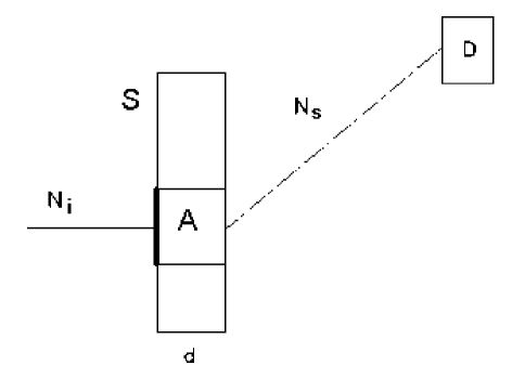
FIG. 1.: Definition of the cross section for scattering on a single atom

Experimentalists divide this value by dimensional parameter $N_{0}d$, where $N_{0}$ is atomic number density in the sample, and $d$ is the sample width. As a result one obtains the cross section

$$\sigma(\mbox{\boldmath$k$}_{i}\to\mbox{\boldmath$k$}_{f})=\frac{N_{s}}{N_{i}N_{0}d}=\frac{N_{s}}{JSN_{0}d}=\frac{N_{s}}{JV},$$ (20)

where $V=Sd$ is the volume of the sample illuminated by the incident neutron flux. The expression (20) is commonly accepted, but gives no insight into interaction of a single neutron with a single atom.

It looks more reasonable from total probability $W(\mbox{\boldmath$k$}_{i}\to\mbox{\boldmath$k$}_{f})$ (19) of scattering of a single neutron in the whole sample to find the scattering probability $w_{1}$ of a single neutron on a single atom:

$$w_{1}(\mbox{\boldmath$k$}_{i}\to\mbox{\boldmath$k$}_{f})=\frac{W(\mbox{\boldmath$k$}_{i}\to\mbox{\boldmath$k$}_{f})}{N_{a}},$$ (21)

where $N_{a}$ is the number of atoms met by a single neutron on its way during the flight through the sample. To find the number of atoms on the neutron’s way we have to introduce a front area $A$ of the incident particle wave function, and suppose that scattering takes place only, if the scattering center crosses this area. So, let the neutron wave function to have area $A$, then $N_{a}=N_{0}Ad$. From (21) we immediately find the scattering cross section of a single neutron per single atom:

$$\sigma(\mbox{\boldmath$k$}_{i}\to\mbox{\boldmath$k$}_{f})=Aw_{1}(\mbox{\boldmath$k$}_{i}\to\mbox{\boldmath$k$}_{f})=\frac{W(\mbox{\boldmath$k$}_{i}\to\mbox{\boldmath$k$}_{f})}{N_{0}d}=\frac{N_{s}}{N_{i}N_{0}d}=\frac{N_{s}}{JSN_{0}d}=\frac{N_{s}}{JN_{0}V},$$ (22)

which coincides with (20). The left hand side is the cross section we must calculate, the right hand side is the experimentally defined cross section. To compare theory with experiment we must be able to calculate $w_{1}(\mbox{\boldmath$k$}_{i}\to\mbox{\boldmath$k$}_{f})$ and $A$.

B Phenomenological definition of the scattering cross section

According to all the textbooks the scattering cross section is defined as a ratio of the count rate $N_{s}$ of scattered particles to the flux density, $J$, of the incident particles:

$$\sigma=\frac{N_{s}}{J}.$$ (23)

If, for instance, we have a small sample, the above ratio gives the cross section of the whole sample, and if we divide this ratio by the total number of atoms in the sample, $N_{a}=N_{0}V$, illuminated by the incident flux, we obtain the result (20), which defines the cross section per one atom. We call it a phenomenological definition, because it says nothing about interaction of a single neutron with a single atom.

C Theoretical definition of the scattering cross section

Theoretically, if you want to find a number of scattered particles for a single target atom and a given incident flux $J$, you must first find, how a single particle is scattered, and how this scattering depends on impact parameter. After that we should integrate over all particles in the incident flux, and average over all possible positions of the scatterer. This procedure gives the number $N_{s}$ of scattered particles for the given $J$. The ratio $N_{s}/J$ is an average cross section $Aw_{1}$, and it can be compared with the phenomenological one.

The parameter $A$ includes also dimension of a single nucleus. We can even suppose that it is related only to nucleus, and neutrons are point particles, propagating like rays of a wave. In that case $A$ is equal to the size $\sigma_{N}$ of the nucleus, and the total cross section can never be larger than $\sigma_{N}$, because the total probability $w_{1}$ can never be larger than unity. This contradicts to the well known facts, that some capture cross sections can be many orders of magnitude larger than $\sigma_{N}$. To avoid this contradiction, we have to assume that $A$ is related to neutron and is considerably larger than $\sigma_{N}$, so we can neglect contribution of $\sigma_{N}$ into $A$.

D On wave packets

Introduction of the finite front area means that the particle wave function is not a plane wave, but a wave packet. This wave packet cannot be spreading, because, if it were, the transmission of a sample would decrease, when the sample is shifted from source to detector, and no one, so far, had ever observed such a phenomenon.

One of the possible candidates for the nonspreading wave packet is the singular de Broglie wave packet (dBWP) [6, 7, 8]

$$\psi_{dB}(\mbox{\boldmath$r$},\mbox{\boldmath$v$},t,s)=\sqrt{\frac{s}{2\pi}}\exp(i\mbox{\boldmath$k$}\mbox{\boldmath$r$}-i\omega(k,s)t)\frac{\exp(-s|\mbox{\boldmath$r$}-\mbox{\boldmath$v$}t|)}{|\mbox{\boldmath$r$}-\mbox{\boldmath$v$}t|},$$ (24)

where $\omega(k,s)=[k^{2}-s^{2}]/2$, $s$ determines the packet width, and $v$ is the wave packet velocity, which in our units $m=\hbar=1$ coincides with wave vector $k$. The front area of (24) can be estimated as $A_{dB}=\pi/s^{2}$. Some reasonings related to solution of ultra cold neutrons anomaly [7], leads to

$$s\approx 3\cdot 10^{-5}k,$$ (25)

which means that for thermal energies $A_{dB}\gg\sigma_{N}$. Because of that the short range interaction becomes a long range one, which is manifested in such effects as total reflection and diffraction in crystals. For description of these processes one does not use cross sections, so the parameter $A$ can be even omitted, and neutrons can be represented by plane waves.

III Three scattering theories

At present we have three theories and every one has its own drawbacks.

  SHT.

It is used only for elastic scattering and two particles scattering in CM reference frame. It is logically inconsistent and contradicts to canonical quantum mechanics (CQM), because it does not describe free particles after scattering. The spherical waves are not solutions of the free Schrödinger equation. To make SHT self consistent one have to find asymptotical form of spherical waves, which is a superposition of free states or free plane waves. However after this step no cross section appears in theory, but only dimensionless probabilities.

  SST.

This theory, which uses Van Hove correlation functions, is not a theory, but only a set of rules how to calculate a cross section. This “theory” uses free states after scattering, however it never calculates scattering amplitudes, operates with probability per unit time, which does not depend on time, introduces superfluous space cell of arbitrary large size $L$, a flux density for a single particle and has other drawbacks discussed below.

  FST.

Its main goal is to justify SST. It uses asymptotical wave function after scattering, which is a superposition of free states. More over it calculates scattering probabilities. However these probabilities violate unitarity, and transition from probabilities to cross sections contains some connivance, which is not valid.

Now we shall consider them in details

A Theory of spherical harmonics (SHT)

In this theory the wave function of a scattered neutron is represented (see, for example, [1]) as

$$\Psi=\exp(i\mbox{\boldmath$k$}\mbox{\boldmath$r$})-\frac{f(\vartheta)}{r}\exp(ikr),$$ (26)

where plane $\exp(i\mbox{\boldmath$k$}\mbox{\boldmath$r$})$ and spherical $\exp(ikr)/r$ waves describe incident and scattered particles, respectively. The scattering amplitude is

$$f(\vartheta)=\frac{1}{2ik}\sum\limits_{l=0}^{\infty}(2l+1)(S_{l}-1)P_{l}(\cos\vartheta)$$ (27)

where $S_{l}$ are scattering matrix elements of spherical harmonics and $P_{l}(\cos\vartheta)$ are Legeandre polynomials.

The simplest process is elastic s-wave scattering from a fixed center with wave function,

$$\Psi=\exp(i\mbox{\boldmath$k$}\mbox{\boldmath$r$})-\frac{b}{r}\exp(ikr),$$ (28)

in which $f(\vartheta)=b=$const.

The approach with spherical waves is borrowed from classical theories of sound and classical light scattering, but it is not a quantum scattering theory, because the spherical wave does not describe a free particle. It satisfies the equation

$$[\Delta+k^{2}]\frac{\exp(ikr)}{r}=-4\pi\delta(\mbox{\boldmath$r$}),$$ (29)

with the right hand side containing the Dirac $\delta$-function. It is not identical zero in the whole space. Therefore (29) is not a free equation. Usually one says that we need wave function outside the point $r=0$, and there the spherical wave satisfies the free Schrödinger equation. However even the wave function of the bound state does satisfy free Schrödinger equation outside the potential. Nevertheless we do not consider the tails of the bound wave functions as free particles. Of course, in the case of bound states the wave function tails decay exponentially at infinity, and this fact justifies why these tails are not considered as free particles. We shall show below, that the asymptotic $1/r$ of spherical waves also contains exponentially decaying waves. Therefore to get real asymptotic of spherical waves at infinity we need to exclude exponentially decaying part from it too (compare (32) and (33) below).

To make SHT really quantum theory we have to find asymptotical form of spherical waves, when particles are sufficiently separated after scattering. This asymptotical wave function should be a superposition

$$\Psi\Rightarrow\exp(i\mbox{\boldmath$k$}\mbox{\boldmath$r$})-\int d\Omega F^{\prime}(k,\Omega)\exp(i\mbox{\boldmath$k$}_{\Omega}\mbox{\boldmath$r$}),$$ (30)

where $\mbox{\boldmath$k$}_{\Omega}$ is wave vector of the length $|\mbox{\boldmath$k$}_{\Omega}|=|\mbox{\boldmath$k$}|$ pointing into the direction $\Omega$ in the element $d\Omega$ of the solid angle $\Omega$. Then the probability of scattering into $d\Omega$ is

$$dw(k,\Omega)=|F^{\prime}(k,\Omega)|^{2}d\Omega.$$ (31)

The asymptotic wave function (30) can be found in two ways: stationary and nonstationary ones.

1 The stationary way

The spherical function has 2-dimensional Fourier expansion

$$\frac{\exp(ikr)}{r}=\frac{i}{2\pi}\int\exp(i\mbox{\boldmath$p$}_{\|}\mbox{\boldmath$r$}_{\|}+ip_{z}|z|)\frac{d^{2}p_{\|}}{p_{z}},$$ (32)

where we fix the direction from the scatterer to the observation point as $z$-axis, and integrate over all components $\mbox{\boldmath$p$}_{\|}$ parallel to $x,y$ plane with $z$-component of the momentum being equal to $p_{z}=\sqrt{k^{2}-p_{\|}^{2}}$.

The range of integration over $\mbox{\boldmath$p$}_{\|}$ (32) is infinite, and, in particular, it includes those $\mbox{\boldmath$p$}_{\|}$, for which $p_{\|}^{2}>k^{2}$. At these $\mbox{\boldmath$p$}_{\|}$ the component $p_{z}$ is imaginary, and $\exp(ip_{z}|z|)$ is an exponentially decaying function. If the distance to the observation point is large enough (later we discuss what does it mean “enough”), we can neglect exponentially decaying terms, and restrict integration to $p_{\|}^{2}\leq k^{2}$:

$$\frac{\exp(ikr)}{r}\approx\frac{i}{2\pi}\int\limits_{p_{\|}^{2}<k^{2}}\exp(i\mbox{\boldmath$p$}_{\|}\mbox{\boldmath$r$}+ip_{z}|z|)\frac{d^{2}p_{\|}}{p_{z}}.$$ (33)

In this integral we can substitute

$$\frac{d^{2}p_{\|}}{p_{z}}=d^{3}p\delta(p^{2}/2-k^{2}/2)\Theta(p_{z}z>0),$$ (34)

where $p^{2}=p_{\|}^{2}+p_{z}^{2}$, $p_{z}$ is a variable, and we introduced the step function $\Theta(x)$, which is unity or zero, when inequality in its argument is satisfied or not, respectively. Substitution of (34) into (33) gives

$$\frac{\exp(ikr)}{r}\approx\frac{i}{2\pi}\int\limits\exp(i\mbox{\boldmath$p$}\mbox{\boldmath$r$})\Theta(p_{z}z>0)\,d^{3}p\delta(p^{2}/2-k^{2}/2)=\frac{ik}{2\pi}\int\limits_{4\pi}\exp(i\mbox{\boldmath$k$}_{\Omega}\mbox{\boldmath$r$})d\Omega,$$ (35)

The terms which we neglected are of the order $1/r$ because at the observation point $z$ ($\mbox{\boldmath$r$}_{\|}=0$) we have

$$\frac{1}{2\pi}\left|\int\limits_{p_{\|}^{2}>k^{2}}\exp\left(-\sqrt{p_{\|}^{2}-k^{2}}z\right)\frac{d^{2}p_{\|}}{\sqrt{p_{\|}^{2}-k^{2}}}\right|=\frac{1}{r},$$ (36)

where we replaced $z$ by the distance $r$ between scatterer and observation point.

Thus the asymptotical form of the wave function (28) after scattering is just (30) with scattering probability amplitude

$$F^{\prime}(k,\Omega)=\frac{ibk}{2\pi}=i\frac{b}{\lambda},$$ (37)

and scattering probability

$$dw(k,\Omega)=|F^{\prime}(k,\Omega)|^{2}d\Omega=\left|\frac{b}{\lambda}\right|^{2}d\Omega,\quad w(k)=\int\limits_{4\pi}dw(k,\Omega)=4\pi\left|\frac{b}{\lambda}\right|^{2},$$ (38)

where $\lambda=2\pi/k$ is the neutron wave length. We see that (28) is reduced to (30), when we neglect the terms of the order $b/r$. Since the decision to neglect or not to neglect this term is at will of the physicist, then the distance $r$ from the center is not an asymptotical one, being even of light years size, if he uses the spherical wave. On the other side the distances of the order 1 Å are asymptotical ones, if $b/r$ is neglected.

2 The nonstationary derivation of asymptotical wave function at large times $t\to\infty$

To find nonstationary asymptotic of the wave function (28) we include in it the time dependent factor $\exp(-i\omega_{k}t)$, where $\omega_{k}=k^{2}/2$, and use 3-dimensional Fourier expansion for the spherical wave

$$\delta\psi(r,t)=\frac{b}{r}\exp(ikr-i\omega_{k}t)=\frac{b}{(2\pi)^{2}}\int\limits\frac{d^{3}p}{\omega_{p}-\omega_{k}-i\epsilon}\exp(i\mbox{\boldmath$p$}\mbox{\boldmath$r$}-i\omega_{k}t),\qquad\quad\omega_{p}=p^{2}/2.$$ (39)

One adds and subtracts $i\omega_{p}t$ in the exponent, and represents the field (39) as a superposition of plane waves

$$\delta\psi=\int\limits\widetilde{F}^{\prime}(\mbox{\boldmath$p$},t)\exp(i\mbox{\boldmath$p$}\mbox{\boldmath$r$}-i\omega_{p}t)d^{3}p,$$ (40)

with amplitudes

$$\widetilde{F}^{\prime}(\mbox{\boldmath$p$},t)=\frac{b}{(2\pi)^{2}}\frac{\exp(i[\omega_{p}-\omega_{k}]t)}{\omega_{p}-\omega_{k}-i\epsilon},$$ (41)

which depend on time $t$.

There is a relation [4]

$$\frac{\exp(i[\omega_{p}-\omega_{k}]t)}{\omega_{p}-\omega_{k}-i\epsilon}=i\int\limits_{-\infty}^{t}\exp(i[\omega_{p}-\omega_{k}]t^{\prime})dt^{\prime},$$ (42)

which in the limit $t\to\infty$ gives the law of energy conservation:

$$i\lim\limits_{t\to\infty}\int\limits_{-\infty}^{t}\exp(i[\omega_{p}-\omega_{k}]t^{\prime})dt^{\prime}=2\pi i\delta(\omega_{p}-\omega_{k})=4\pi i\delta(p^{2}-k^{2}).$$ (43)

In this limit (40) is

$$\delta\psi=\int\limits\frac{ib}{\pi}\exp(i\mbox{\boldmath$p$}\mbox{\boldmath$r$}-i\omega_{p}t)d^{3}p\delta(p^{2}-k^{2})=\frac{ibk}{2\pi}\int\limits_{4\pi}d\Omega\exp(i\mbox{\boldmath$k$}_{\Omega}\mbox{\boldmath$r$}-i\omega_{k}t),$$ (44)

and we get dimensionless scattering probability amplitude (37) and the total scattering probability $w(k)=4\pi|b/\lambda|^{2}$, which coincide with (38).

The main result of all these considerations is: the correct asymptotical wave function gives not a cross section, but only dimensionless probability.

3 Phenomenological definition of cross section

With asymptotical wave function (44) it is possible to define phenomenological semi integral cross section $\sigma(\mbox{\boldmath$n$})$ as a ratio of normal flux $J(\mbox{\boldmath$n$})$ through an infinite plane $S(\mbox{\boldmath$n$})$ with normal $n$ to the incident flux density $k$

$$\sigma(\mbox{\boldmath$n$})=\frac{1}{2ik}\int d^{2}r_{\parallel}\left[\delta\psi^{*}(\mbox{\boldmath$r$})\overrightarrow{\frac{d}{dz}}\delta\psi(\mbox{\boldmath$r$})-\delta\psi^{*}(\mbox{\boldmath$r$})\overleftarrow{\frac{d}{dz}}\delta\psi(\mbox{\boldmath$r$})\right].$$ (45)

The wave function (44) in general case, when scattering is nonisotropic ($b=b(\mbox{\boldmath$k$}_{\Omega})$), can be represented as

$$\delta\psi(\mbox{\boldmath$r$})=\frac{ik}{2\pi}\int\limits_{4\pi}d\Omega b(\mbox{\boldmath$k$}_{\Omega})\exp(i\mbox{\boldmath$k$}_{\Omega}\mbox{\boldmath$r$}-i\omega_{k}t)=\frac{i}{2\pi}\int\limits_{p_{\parallel}<k}\frac{d^{2}p_{\parallel}}{p_{\perp}}b(\mbox{\boldmath$p$})\exp(i\mbox{\boldmath$p$}\mbox{\boldmath$r$}-i\omega_{k}t),$$ (46)

where $p_{\perp}=\sqrt{k^{2}-p^{2}_{\parallel}}$. Substitution of this function into (45) gives

$$\sigma(\mbox{\boldmath$n$})=\int\limits_{p_{\parallel}<k}\frac{d^{2}p_{\parallel}}{kp_{\perp}}|b(\mbox{\boldmath$p$})|^{2}=\int\limits_{2\pi(\mbox{\boldmath$n$})}|b(\mbox{\boldmath$k$}_{\Omega})|^{2}d\Omega,$$ (47)

where $2\pi(\mbox{\boldmath$n$})$ denotes solid angle $2\pi$ around normal vector $n$. We can define differential cross section as

$$\frac{d\sigma}{d\Omega}=\frac{d\sigma(\mbox{\boldmath$n$})}{d\mbox{\boldmath$n$}}=|b(\mbox{\boldmath$k$}_{\Omega})|^{2}.$$ (48)

This definition is not unique, because some arbitrary function $F(\Omega)$ can be added to it, for which

$$\int\limits_{2\pi}F(\Omega)d\Omega=0,$$

and we do not want to accept it, because it is a phenomenological one.

B The Standard Scattering Theory (SST)

SST (see, for example [2, 3]) is more general than SHT, because it is applied to both elastic and inelastic processes. It lists the rules, to be justified by FST, one must use to derive scattering cross section. These rules are:

1. Define the cross section as a ratio

   $$d\sigma=\frac{1}{J_{i}}dW_{F},$$ (49)

   where $J_{i}$ is the flux density of incident neutrons, and $dW_{F}$ is probability of scattering per unit time:

2. Define the probability of scattering per unit time according to the Fermi Golden Rule

   $$dW_{F}(\mbox{\boldmath$k$}_{i},\lambda_{i}\to\mbox{\boldmath$k$}_{f},\lambda_{f},t)=\frac{2\pi}{\hbar}\left|\langle\lambda_{f},\mbox{\boldmath$k$}_{f}|V|\lambda_{i},\mbox{\boldmath$k$}_{i}\rangle\right|^{2}\rho(E_{fk}),$$ (50)

   where $\langle\lambda_{f},\mbox{\boldmath$k$}_{f}|V|\lambda_{i},\mbox{\boldmath$k$}_{i}\rangle$ is a matrix element of the neutron-scatterer interaction potential $V$ between initial $|\mbox{\boldmath$k$}_{i}>$, $|\lambda_{i}>$, and final $|\mbox{\boldmath$k$}_{f}>$, $|\lambda_{f}>$, neutron and scatterer states, respectively, and $\rho(E_{fk})$ is the density of the neutron final states:

   $$\rho(E_{fk})=\delta(E_{ik}+E_{i\lambda}-E_{fk}+E_{f\lambda})\frac{L^{3}d^{3}k_{f}}{(2\pi)^{3}}.$$ (51)

   The delta-function factor corresponds to the energy conservation law. It contains initial and final neutron $E_{i,fk}$ and scatterer $E_{i,f\lambda}$ energies. The last factor is the phase space density of the neutron final states, which includes momentum element $d^{3}k_{f}$ and some volume $L^{3}$ with an arbitrary large size $L$.

3. Define neutron states before and after scattering as (they are really free states)

   $$|\mbox{\boldmath$k$}_{i}>=L^{-3/2}\exp(i\mbox{\boldmath$k$}_{i,f}\mbox{\boldmath$r$}),$$ (52)

   and with them the flux density of the incident neutron

   $$J_{i}=\hbar\frac{k_{i}}{L^{3}}.$$ (53)

4. The ratio (49) gives the cross section

   $$d\sigma(\mbox{\boldmath$k$}_{i},\lambda_{i}\to\mbox{\boldmath$k$}_{f},\lambda_{f})=\frac{2\pi m}{\hbar^{2}k_{i}}\left|\langle\lambda_{f},\mbox{\boldmath$k$}_{f}|V|\lambda_{i},\mbox{\boldmath$k$}_{i}\rangle\right|^{2}\delta(E_{ik}+E_{i\lambda}-E_{fk}+E_{f\lambda})\frac{L^{6}d^{3}k_{f}}{(2\pi)^{3}}.$$ (54)

   Taking into account that $E_{fk}=\hbar^{2}k_{f}^{2}/2m$, $d^{3}k_{f}=mk_{f}dE_{f}d\Omega_{f}/\hbar^{2}$, one obtains double differential scattering cross section

   $$\frac{d^{2}\sigma}{dE_{f}d\Omega_{f}}(\mbox{\boldmath$k$}_{i},\lambda_{i}\to\mbox{\boldmath$k$}_{f},\lambda_{f})=\frac{m^{2}k_{f}}{\hbar^{4}k_{i}}\left|\langle\lambda_{f},\mbox{\boldmath$k$}_{f}|V|\lambda_{i},\mbox{\boldmath$k$}_{i}\rangle\right|^{2}\delta(E_{ik}+E_{i\lambda}-E_{fk}+E_{f\lambda})\frac{L^{6}}{(2\pi)^{2}}.$$ (55)

   To compare with experimentally measured value one averages (55) over initial states and sums over final states of the scatterer, getting

   $$\frac{d^{2}\sigma}{dE_{f}d\Omega_{f}}(\mbox{\boldmath$k$}_{i}\to\mbox{\boldmath$k$}_{f},{\cal P})=$$

   $$\sum\limits_{\lambda_{i},\lambda_{f}}{\cal P}(\lambda_{i})\frac{m^{2}k_{f}}{\hbar^{4}k_{i}}\left|\langle\lambda_{f},\mbox{\boldmath$k$}_{f}|V|\lambda_{i},\mbox{\boldmath$k$}_{i}\rangle\right|^{2}\delta(E_{ik}+E_{i\lambda}-E_{fk}+E_{f\lambda})\frac{L^{6}}{(2\pi)^{2}},$$ (56)

   where ${\cal P}(\lambda_{i})$ is the probability of scatterer to be initially in the state $|\lambda_{i}\rangle$.

In the case, when

$$V=\frac{\hbar^{2}}{2m}4\pi b\delta(\mbox{\boldmath$r$}_{n}-\mbox{\boldmath$r$}_{s}),$$

where $\delta$-function depends on neutron and scatterer positions $\mbox{\boldmath$r$}_{n}$, $\mbox{\boldmath$r$}_{s}$ respectively, the cross section (56) becomes

$$\frac{d^{2}\sigma}{dE_{f}d\Omega_{f}}(\mbox{\boldmath$k$}_{i}\to\mbox{\boldmath$k$}_{f},{\cal P})=\sum\limits_{\lambda_{i},\lambda_{f}}{\cal P}(\lambda_{i})\frac{k_{f}}{k_{i}}\left|\langle\lambda_{f}|\exp(i\mbox{\boldmath$\kappa$}\mbox{\boldmath$r$}_{s})|\lambda_{i}\rangle\right|^{2}\delta(E_{ik}+E_{i\lambda}-E_{fk}+E_{f\lambda}),$$ (57)

where $\mbox{\boldmath$\kappa$}=\mbox{\boldmath$k$}_{i}-\mbox{\boldmath$k$}_{f}$ is momentum transferred to the scatterer.

One of contradictions here is that the probability of scattering per unit time (50) does not depend on time, so integral of $dW_{F}$ over time is senseless, whereas according definition it should be less than unity.

Two other dubious points are: introduction of the superfluous volume $L^{3}$ and of flux density for a single particle.

The SST has also another drawback — one never calculates scattering amplitude in it. However this amplitude can be important. With it one would be able to find coherent amplitude, which is averaged over initial states $|\lambda_{i}\rangle$ of the scatterer. This amplitude gives coherent scattering cross section, which some times could carry an additional information about scattering process.

C The Fundamental Scattering Theory (FST)

In FST (see, for example [4, 5]), which was developed mainly to justify SST, the scattering process is divided into three stages: infinite past, where incident particle is free; present, where the neutron interacts with a scatterer; and infinite future, where scattered neutron is again a free particle. To work within the Hilbert space of normalized states, the incident free neutron is represented by a wave packet $|\phi\rangle$ with Fourier expansion:

$$|\phi\rangle\equiv|\phi(\mbox{\boldmath$k$},s)\rangle=\int\limits d^{3}pa(\mbox{\boldmath$k$}-\mbox{\boldmath$p$},s)|\mbox{\boldmath$p$}\rangle,$$ (58)

where parameter $s$ characterizes dimension of the wave packet, $k$ is momentum of the packet, $|\mbox{\boldmath$p$}\rangle$ is a state corresponding to plane wave, $\langle\mbox{\boldmath$r$}|\mbox{\boldmath$p$}\rangle=\exp(i\mbox{\boldmath$p$}\mbox{\boldmath$r$})$, in coordinate space, and $a(\mbox{\boldmath$p$})$ are numerical Fourier coefficients. The dynamics of the packet $|\phi\rangle$ is determined by free hamiltonian $H_{0}$:

$$|\phi(t)\rangle=\exp(-iH_{0}t)|\phi\rangle.$$ (59)

After scattering the wave function becomes

$$|\chi\rangle=\int\limits d^{3}p^{\prime}|\mbox{\boldmath$p$}^{\prime}\rangle\int\limits d^{3}p\langle\mbox{\boldmath$p$}^{\prime}|\hat{S}|\mbox{\boldmath$p$}\rangle a(\mbox{\boldmath$k$}-\mbox{\boldmath$p$},s),$$ (60)

where $\hat{S}$ is scattering matrix. And dimensionless probability of scattering is defined as

$$dw(\mbox{\boldmath$k$}\to\mbox{\boldmath$p$}^{\prime})=d^{3}p^{\prime}|\langle\mbox{\boldmath$p$}^{\prime}||\chi\rangle|^{2}=d^{3}p^{\prime}\left|\int\limits d^{3}p\langle\mbox{\boldmath$p$}^{\prime}|\hat{S}|\mbox{\boldmath$p$}\rangle a(\mbox{\boldmath$k$}-\mbox{\boldmath$p$},s)\right|^{2}.$$ (61)

This last formula is absolutely wrong. It means that scattering transforms the wave packet into a plane wave. Such a process is impossible because it completely violates unitarity. The state $|\phi\rangle$ is normalized and $|\mbox{\boldmath$p$}\rangle$ is not normalizable.

From unitarity of the $S$-matrix it follows that norm of the wave function is preserved. So the final wave function $|\chi\rangle$ after scattering is ether a wave packet or a superposition of wave packets

$$|\chi\rangle=\int\limits d^{3}k^{\prime}b(\mbox{\boldmath$k$}\to\mbox{\boldmath$k$}^{\prime})|\phi(\mbox{\boldmath$k$}^{\prime},s^{\prime})\rangle$$ (62)

with some new $s^{\prime}$ if the parameter $s$ depends on $k$. Then $b(\mbox{\boldmath$k$}\to\mbox{\boldmath$k$}^{\prime})=\langle\phi(\mbox{\boldmath$k$}^{\prime},s^{\prime})|\hat{S}|\phi(\mbox{\boldmath$k$},s)\rangle$ defines the amplitude of transition probability of the wave packet state $|\phi(\mbox{\boldmath$k$},s)\rangle$ with momentum $k$ into the wave packet state $|\phi(\mbox{\boldmath$k$}^{\prime},s^{\prime})\rangle$ with momentum $\mbox{\boldmath$k$}^{\prime}$.

In fact, in the books [4, 5] and others only scattering of plane waves is considered, and the initial wave packet defines only spectrum of plane waves in the incident beam. However plane waves scattering gives only probability, and averaging over initial spectrum of plane waves does not change the situation.

In FST one also introduces the finite volume $L^{3}$ with an arbitrary large $L$ for justification of SST. Below we show that it is possible to avoid this artificial step. We use fundamental scattering theory with plane waves (FPWST) and calculate scattering probability of neutron in monatomic gas. This probability, as is shown in introduction, is ambiguous, however, on one side, there is a way to find the standard expression for cross section, and on the other side, knowledge of the ambiguity helps to find the way to fight it.

The authors of [4, 5] and other books, make one special step to get cross section from probability, however this step contains a connivance that there is no scattering, if the scatterer does not cross the neutron wave packet. In linear scattering theory it is false, as we shall see in section 5. Nevertheless we shall accept this point, because otherwise it is absolutely impossible to get a cross section from probability. We shall accept such a connivance as an implicit introduction of nonlinearity into neutron-atom interaction.

IV Direct calculation of neutron scattering from a monatomic gas

Here we apply the principles of FST to plane wave neutron-atom scattering and show that the result is ambiguous. We also show how one can obtain the known result of SST.

A The scattering amplitude (1)

When we consider neutron scattering from a monatomic gas, we must treat the neutron and atom of the gas in the same way, it means that we need the same Schrödinger equation for both particles

$$\left[i\frac{\partial}{\partial t}+\frac{\Delta_{n}}{2}+\frac{\mu\Delta_{a}}{2}-\frac{1}{2}u(\mbox{\boldmath$r$}_{n}-\mbox{\boldmath$r$}_{a},t)\right]\psi(\mbox{\boldmath$r$}_{n},\mbox{\boldmath$r$}_{a},t)=0,$$ (63)

where potential $u$ is

$$u(\mbox{\boldmath$r$},t)=4\pi b\delta(\mbox{\boldmath$r$}_{n}-\mbox{\boldmath$r$}_{a}),$$ (64)

$\mbox{\boldmath$r$}_{n}$, $\mbox{\boldmath$r$}_{a}$, $m$, $M$ are coordinates and masses of the neutron and atom respectively, $\mu=m/M$, and the time $t$ contains factor $\hbar/m$.

The Green function of equation (63) with excluded interaction is

$$G(\mbox{\boldmath$r$}_{n}-\mbox{\boldmath$r$}^{\prime}_{n},\mbox{\boldmath$r$}_{a}-\mbox{\boldmath$r$}^{\prime}_{a},t-t^{\prime})=\int\limits\frac{\exp(i\mbox{\boldmath$k$}_{f}(\mbox{\boldmath$r$}_{n}-\mbox{\boldmath$r$}^{\prime}_{n})+\mbox{\boldmath$p$}_{f}(\mbox{\boldmath$r$}_{a}-\mbox{\boldmath$r$}^{\prime}_{a})-i\omega(t-t^{\prime}))}{E_{fk}+E_{fp}-\omega-i\epsilon}\frac{d^{3}k_{f}d^{3}p_{f}d\omega}{(2\pi)^{7}},$$ (65)

where $E_{fk}=k_{f}^{2}/2$, $E_{fp}=\mu p_{f}^{2}/2$. It can be easily checked by substitution that $G$ satisfies the equation

$$\left[i\frac{\partial}{\partial t}+\frac{\Delta_{n}}{2}+\frac{\mu\Delta_{a}}{2}\right]G(\mbox{\boldmath$r$}_{n}-\mbox{\boldmath$r$}^{\prime}_{n},\mbox{\boldmath$r$}_{a}-\mbox{\boldmath$r$}^{\prime}_{a},t-t^{\prime})=-\delta(\mbox{\boldmath$r$}_{n}-\mbox{\boldmath$r$}_{n}^{\prime})\delta(\mbox{\boldmath$r$}_{a}-\mbox{\boldmath$r$}_{a}^{\prime})\delta(t-t^{\prime}).$$ (66)

The scattered part of the wave function is

$$\delta\psi=\frac{2\pi b}{(2\pi)^{7}}\int\limits\frac{d^{3}k_{f}d^{3}p_{f}d\omega d^{3}r^{\prime}_{n}d^{3}r^{\prime}_{a}dt^{\prime}}{E_{fk}+E_{fp}-\omega-i\epsilon}\exp(i\mbox{\boldmath$k$}_{f}(\mbox{\boldmath$r$}_{n}-\mbox{\boldmath$r$}^{\prime}_{n})+i\mbox{\boldmath$p$}_{f}(\mbox{\boldmath$r$}_{a}-\mbox{\boldmath$r$}^{\prime}_{a})-i\omega(t-t^{\prime}))\times$$

$$\delta(\mbox{\boldmath$r$}^{\prime}_{n}-\mbox{\boldmath$r$}^{\prime}_{a})\exp(i\mbox{\boldmath$k$}_{i}\mbox{\boldmath$r$}^{\prime}_{n}+i\mbox{\boldmath$p$}_{i}\mbox{\boldmath$r$}^{\prime}_{a}-i(E_{ik}+E_{ip})t^{\prime})=$$

$$=\frac{b}{(2\pi)^{2}}\int\limits\frac{d^{3}k_{f}d^{3}p_{f}\delta(\mbox{\boldmath$k$}_{f}+\mbox{\boldmath$p$}_{f}-\mbox{\boldmath$k$}_{i}-\mbox{\boldmath$p$}_{i})}{E_{fk}+E_{fp}-E_{ik}-E_{ip}-i\epsilon}\exp(i\mbox{\boldmath$k$}_{f}\mbox{\boldmath$r$}_{n}+i\mbox{\boldmath$p$}_{f}\mbox{\boldmath$r$}_{a}-i(E_{ik}+E_{ip})t),$$ (67)

where $\exp(i\mbox{\boldmath$k$}_{i}\mbox{\boldmath$r$}_{n}-iE_{ik}t)$, $\exp(i\mbox{\boldmath$p$}_{i}\mbox{\boldmath$r$}_{a}-iE_{ip}t)$ describe incident plane waves of the neutron and atom respectively with their energies $E_{ik}=k_{i}^{2}/2$, and $E_{ip}=\mu p_{i}^{2}/2$.

The wave function (67) after integration over $\mbox{\boldmath$p$}_{f}$ and $\mbox{\boldmath$k$}_{f}$ can be found in the final form

$$\delta\psi=\frac{b}{1+\mu}\frac{1}{|\mbox{\boldmath$r$}_{n}-\mbox{\boldmath$r$}_{a}|}\exp\left(\frac{i}{1+\mu}[q|\mbox{\boldmath$r$}_{n}-\mbox{\boldmath$r$}_{a}|+i\mbox{\boldmath$P$}(\mu\mbox{\boldmath$r$}_{n}-\mbox{\boldmath$r$}_{a})]-iEt\right),$$ (68)

where $q=|\mbox{\boldmath$k$}_{i}-\mu\mbox{\boldmath$p$}_{i}|$ is relative speed of particles, $\mbox{\boldmath$P$}=\mbox{\boldmath$p$}_{i}+\mbox{\boldmath$k$}_{i}$ is their total momentum, and $E=E_{ik}+E_{ip}$ is their total energy. This wave function has a very clear physical interpretation, however it is not an asymptotical one.

To get the asymptotical wave function we represented (67) as a superposition of plane waves related to final states of the neutron, $\exp(i\mbox{\boldmath$k$}_{f}\mbox{\boldmath$r$}_{n}-iE_{fk}t)$, and atom, $\exp(i\mbox{\boldmath$p$}_{f}\mbox{\boldmath$r$}_{a}-iE_{fp}t)$:

$$\delta\psi=\int\limits\widetilde{F}^{\prime}(\mbox{\boldmath$k$}_{i},\mbox{\boldmath$p$}_{i}\to\mbox{\boldmath$k$}_{f},\mbox{\boldmath$p$}_{f},t)d^{3}k_{f}d^{3}p_{f}\exp(i\mbox{\boldmath$k$}_{f}\mbox{\boldmath$r$}_{n}+i\mbox{\boldmath$p$}_{f}\mbox{\boldmath$r$}_{a}-iE_{fk}t-iE_{fp}t),$$ (69)

where

$$\widetilde{F}^{\prime}(\mbox{\boldmath$k$}_{i},\mbox{\boldmath$p$}_{i}\to\mbox{\boldmath$k$}_{f},\mbox{\boldmath$p$}_{f},t)=\frac{b}{(2\pi)^{2}}\frac{\delta(\mbox{\boldmath$k$}_{i}+\mbox{\boldmath$p$}_{f}-\mbox{\boldmath$k$}_{i}-\mbox{\boldmath$p$}_{i})}{E_{fk}+E_{fp}-E_{ik}-E_{ip}-i\epsilon}\exp(i(E_{fk}+E_{fp}-E_{ik}-E_{ip})t).$$ (70)

With the relation (42) we find in the limit $t\to\infty$ that the probability amplitude for the particle to leave in the state $\mbox{\boldmath$k$}_{f}$, and for the atom to leave in the state $\mbox{\boldmath$p$}_{f}$ is:

$$\lim_{t\to\infty}\widetilde{F}^{\prime}(\mbox{\boldmath$k$}_{i},\mbox{\boldmath$p$}_{i}\to\mbox{\boldmath$k$}_{f},\mbox{\boldmath$p$}_{f},t)d^{3}k_{f}d^{3}p_{f}=d^{3}k_{f}d^{3}p_{f}\frac{ib}{2\pi}\delta(\mbox{\boldmath$k$}_{f}+\mbox{\boldmath$p$}_{f}-\mbox{\boldmath$k$}_{i}-\mbox{\boldmath$p$}_{i})\delta(E_{fk}+E_{fp}-E_{ik}-E_{ip}),$$ (71)

which coincides with (1).

B How to get the standard cross section

Now we can show that with this amplitude it is possible to get the standard cross section. For that we transform to CM reference frame and obtain the probability scattering amplitude (13):

$$dF(\mbox{\boldmath$k$}_{i},\Omega_{c},\mbox{\boldmath$p$}_{i})=\frac{ibq}{2\pi(1+\mu)^{2}}d\Omega_{c},$$ (72)

from which with the help of front area $A$ and (14) we obtain the cross section in the CM frame

$$d\sigma(\mbox{\boldmath$k$}_{i},\Omega_{c},\mbox{\boldmath$p$}_{i})=A\left|\frac{ibq}{2\pi(1+\mu)^{2}}\right|^{2}d\Omega_{c}$$ (73)

for neutron scattering on an atom with the initial momentum $\mbox{\boldmath$p$}_{i}$.

Transformation to the laboratory frame according to (12) gives

$$d\tilde{\sigma}_{l}(\mbox{\boldmath$k$}_{i}\to\mbox{\boldmath$k$}_{f},\mbox{\boldmath$p$}_{i})=Aq\left|\frac{ib}{2\pi(1+\mu)}\right|^{2}d^{3}k_{f}\delta(E_{R}-\omega+\mu\mbox{\boldmath$p$}_{i}\mbox{\boldmath$\kappa$}).$$ (74)

The number of collisions per unit time in a gas sample is

$$\nu(\mbox{\boldmath$k$}_{i}\to\mbox{\boldmath$k$}_{f},\mbox{\boldmath$p$}_{i})=qN_{0}d\tilde{\sigma}_{l}(\mbox{\boldmath$k$}_{i}\to\mbox{\boldmath$k$}_{f},\mbox{\boldmath$p$}_{i}),$$

where $q$ is relative velocity. Since the interaction time with the whole sample of width $d$ is $t=d/k_{i}$, then the total probability of a single neutron scattering in the sample is

$$W(\mbox{\boldmath$k$}_{i}\to\mbox{\boldmath$k$}_{f},T)=N_{0}\frac{d}{k_{i}}\int\limits d^{3}p_{i}q\sigma(\mbox{\boldmath$k$}_{i}\to\mbox{\boldmath$k$}_{f},\mbox{\boldmath$p$}_{i}){\cal M}\left(\mu\frac{p_{i}^{2}}{2T}\right),$$

where ${\cal M}(\mu p_{i}^{2}/2T)$ is Maxwellian distribution of $\mbox{\boldmath$p$}_{i}$:

$${\cal M}\left(\frac{\mu p_{i}^{2}}{2T}\right)=\left(\frac{\mu}{2\pi T}\right)^{3/2}\exp\left(-\mu\frac{p_{i}^{2}}{2T}\right).$$

If we accept

$$A=\frac{[2\pi(1+\mu)]^{2}}{q^{2}},$$ (75)

and define cross section as $\sigma=W/N_{0}d$, then we obtain the standard scattering cross section in a monatomic gas

$$d\sigma(\mbox{\boldmath$k$}_{i}\to\mbox{\boldmath$k$}_{f},T)=\frac{|b|^{2}d^{3}k_{f}}{k_{i}\kappa\sqrt{2\pi\mu T}}\exp\left(-\frac{(E_{R}-\omega)^{2}}{4E_{R}T}\right).$$ (76)

It is necessary to point out that definition (75) of the parameter $A$ means that the wave packet contracts with increase of the relative energy, and because of that the wave optics at low energies transforms to geometrical one at high energies.

a The total cross section for an atom at rest.

If instead of Maxwellian distribution we substitute ${\cal M}(\mbox{\boldmath$p$}_{i})=\delta(\mbox{\boldmath$p$}_{i})$, we immediately obtain the total cross section

$$\sigma(\mbox{\boldmath$k$}_{i}\to\mbox{\boldmath$k$}_{f},\mbox{\boldmath$p$}_{i}=0)=4\pi\left|\frac{b}{1+\mu}\right|^{2},$$ (77)

which also coincides with the standard one.

1 Direct calculations in LF

All the standard results were obtained with the help of CM reference frame. If we repeat the same with scattering probability (7) obtained directly in the laboratory reference frame we find a divergency when averaging with Maxwellian distribution and an additional factor

$$Q(\mu)=\frac{8}{3}\mu^{2}+\frac{(1-\mu^{2})^{3/2}}{\mu}\arctan\left(\frac{\mu}{\sqrt{1-\mu^{2}}}\right)$$

in (77) for scattering from an atom at rest.

V About wave packets

Introduction of the parameter $A$ means that instead of plane waves we deal with wave packets. We cannot deduce $A$ from a theory, however we can study its properties. We also need to learn how to describe scattering in terms of wave packets. Here we consider elastic scattering of a wave packet from a fixed center, and find at first sight unexpected though finally well understandable result that probability of scattering does not depend on position of the scattering center. However first of all we need to discuss the types of the wave packets.

A Three types of the wave packets

In general all the wave packets can be represented by their Fourier expansion

$$\psi(\mbox{\boldmath$r$},\mbox{\boldmath$k$},t,s)=G(s|\mbox{\boldmath$r$}-\mbox{\boldmath$k$}t|)\exp(i\mbox{\boldmath$k$}\mbox{\boldmath$r$}-i\omega(k,s)t)=\int\limits d^{3}p\,a(\mbox{\boldmath$p$},\mbox{\boldmath$k$},s)\exp[i\mbox{\boldmath$p$}\mbox{\boldmath$r$}-i\omega(\mbox{\boldmath$p$},\mbox{\boldmath$k$},s)t],$$ (78)

where parameter $s$ determines the width of the packet like in (24), $a(\mbox{\boldmath$p$},\mbox{\boldmath$k$},s)$ and $\omega(\mbox{\boldmath$p$},\mbox{\boldmath$k$},s)$ are functions of invariant variables $\mbox{\boldmath$k$}^{2}$, $\mbox{\boldmath$p$}^{2}$ and $k$$p$.

The primary wave packet describes a free incident particle. Its Fourier expansion contains plane waves $\exp(i\mbox{\boldmath$p$}\mbox{\boldmath$r$})$, which satisfy the equation

$$[\Delta+p^{2}]\exp(i\mbox{\boldmath$p$}\mbox{\boldmath$r$})=0.$$ (79)

All the packets are representable in the form (78), and they differ by the Fourier coefficients $a(\mbox{\boldmath$p$},\mbox{\boldmath$k$},s)$ and dispersion $\omega(\mbox{\boldmath$p$},\mbox{\boldmath$k$},s)$. We consider three types of the wave packets and discuss which one is the most appropriate for description of particles.

1 The Gaussian wave packet

The most popular in the literature is the Gaussian wave packet

$$\psi_{G}(\mbox{\boldmath$r$},\mbox{\boldmath$k$},t,s)=\left(\frac{s}{\sqrt{\pi}(1+its^{2})}\right)^{3/2}e^{i\mbox{\boldmath$k$}\mbox{\boldmath$r$}-ik^{2}t/2}\exp\left(-\frac{s^{2}[\mbox{\boldmath$r$}-\mbox{\boldmath$k$}t]^{2}}{2[1+its^{2}]}\right).$$ (80)

This packet is normalized to unity, satisfies the free Schrödinger equation, but spreads in time. Because of this spreading its form in space does not completely coincides with (78).

Its Fourier components are

$$a_{G}(\mbox{\boldmath$p$},\mbox{\boldmath$k$},s)=\left(\frac{1}{2\pi s\sqrt{\pi}}\right)^{3/2}\exp(-(\mbox{\boldmath$k$}-\mbox{\boldmath$p$})^{2}/2s^{2}),\quad\omega_{G}(\mbox{\boldmath$p$},\mbox{\boldmath$k$},s)=p^{2}/2,$$ (81)

where $s$ is the width in momentum space. The spectrum of wave vectors $p$ is spherically symmetrical with respect to the central point $\mbox{\boldmath$p$}=\mbox{\boldmath$k$}$ and decays away from it according to Gaussian law.

The cross area of this packet moving in $z$ direction can be defined as

$$A_{G}=\int\limits\pi\rho^{2}d^{3}r|\psi_{G}(\mbox{\boldmath$r$},\mbox{\boldmath$k$},t,s)|^{2}=\int\limits\rho^{2}d^{2}\rho\frac{s^{2}}{1+t^{2}s^{4}}\exp\left(-\frac{s^{2}\rho^{2}}{1+t^{2}s^{4}}\right)=\pi\frac{1+t^{2}s^{4}}{s^{2}},$$ (82)

where $\rho=\sqrt{x^{2}+y^{2}}$.

2 Nonsingular de Broglie wave packet

It is known that there are no nonspreading normalizable wave packets, which satisfy the free Schrödinger equation. However nonnormalizable wave packets do exist. As an example we can demonstrate nonsingular de Broglie wave packet [6]

$$\psi_{ns}(\mbox{\boldmath$r$},\mbox{\boldmath$k$},t,s)=\exp(i\mbox{\boldmath$k$}\mbox{\boldmath$r$}-i\omega(k,s)t)j_{0}(s|\mbox{\boldmath$r$}-\mbox{\boldmath$v$}t|),$$ (83)

in which $\omega(k,s)=k^{2}/2+s^{2}/2$ and $\mbox{\boldmath$v$}=\mbox{\boldmath$k$}$ in units $\hbar/m=1$. The packet (83) is a spherical Bessel function $j_{0}(sr)\exp(-is^{2}t/2)$, which center is moving with the speed $v$. This packet satisfy the free Schrödinger equation. Its Fourier components are

$$a_{ns}(\mbox{\boldmath$p$},\mbox{\boldmath$k$},s)\propto\delta((\mbox{\boldmath$k$}-\mbox{\boldmath$p$})^{2}-s^{2}),\quad\omega_{ns}(\mbox{\boldmath$p$},\mbox{\boldmath$k$},s)=p^{2}/2,$$ (84)

and spectrum of $p$ is a sphere of radius $s$ in momentum space with center at the point $\mbox{\boldmath$p$}=\mbox{\boldmath$k$}$. Since it is not normalizable, its front area is infinite, and such a wave packet is not a good candidate for description of free neutrons.

3 The singular de Broglie wave packet

The singular de Broglie wave packet [6]

$$\psi_{dB}(\mbox{\boldmath$r$},\mbox{\boldmath$k$},t,s)=C\exp(i\mbox{\boldmath$k$}\mbox{\boldmath$r$}-i\omega(k,s)t)\frac{\exp(-s|\mbox{\boldmath$r$}-\mbox{\boldmath$v$}t|)}{|\mbox{\boldmath$r$}-\mbox{\boldmath$v$}t|},$$ (85)

is normalizable one with normalization constant $C=\sqrt{s/2\pi}$ defined by

$$\displaystyle\int d^{3}r|{\mit\psi}_{dB}(\mbox{\boldmath$r$},\mbox{\boldmath$k$},t,s)|^{2}=1.$$ (86)

The parameter $s$ is the width of the packet in momentum space and reciprocal width in coordinate space, $\mbox{\boldmath$v$}\equiv\mbox{\boldmath$k$}$ is the packet speed, and $\omega(k,s)=(k^{2}-s^{2})/2$. We see that $\omega(k,s)$ is less than kinetic energy by the term $s^{2}/2$, which can be thought of as bound energy of the packet.

The singular de Broglie wave packet satisfies inhomogeneous Schrödinger equation

$$\left[i\frac{\partial}{\partial t}+\frac{\Delta}{2}\right]\psi_{dB}(\mbox{\boldmath$r$},\mbox{\boldmath$v$},t,s)=-2\pi Ce^{i(v^{2}+s^{2})t/2}\delta(\mbox{\boldmath$r$}-\mbox{\boldmath$v$}t),$$ (87)

with right hand side being zero everywhere except one point.

The Fourier coefficients of the singular de Broglie wave packet are

$$a_{dB}(\mbox{\boldmath$p$},\mbox{\boldmath$k$},s)=\sqrt{\frac{s}{2\pi}}\frac{4\pi}{(2\pi)^{3}}\frac{1}{(\mbox{\boldmath$p$}-\mbox{\boldmath$k$})^{2}+s^{2}}.$$ (88)

and

$$\omega_{dB}(\mbox{\boldmath$p$},\mbox{\boldmath$k$},s)=[2\mbox{\boldmath$k$}\mbox{\boldmath$p$}-k^{2}+s^{2}]/2=[p^{2}-(\mbox{\boldmath$k$}-\mbox{\boldmath$p$})^{2}-s^{2}]/2.$$ (89)

The spectrum of wave vectors $p$ is spherically symmetrical with respect to the central point $\mbox{\boldmath$p$}=\mbox{\boldmath$k$}$ and decays away from it according to Lorenzian law with width $s$.

The Fourier coefficients (88) and frequency (89) become identical to those of spherical wave

$$\exp(-ik^{2}t/2)\frac{\exp(ikr)}{r}=\frac{4\pi}{(2\pi)^{3}}\int\limits\exp(i\mbox{\boldmath$p$}\mbox{\boldmath$r$})\frac{\exp(-ik^{2}t/2)\,d^{3}p}{p^{2}-k^{2}-i\epsilon},$$ (90)

after substitution $\mbox{\boldmath$k$}\to 0$ and $s\to-ik$, i.e. $\psi_{dB}(\mbox{\boldmath$r$},0,t,-ik)=C\exp(ikr-ik^{2}t/2)/r$.

The front area of the singular de Broglie wave packet, moving in $z$ direction can be defined as

$$A_{dB}=\int\pi\rho^{2}d^{3}r|\psi_{dB}(\mbox{\boldmath$r$},\mbox{\boldmath$v$},t,s)|^{2}=\frac{s}{2\pi}\int\limits_{0}^{\infty}2dz\pi d\rho^{2}\pi\rho^{2}\frac{\exp(-2s\sqrt{\rho^{2}+z^{2}})}{\rho^{2}+z^{2}},$$ (91)

where $\rho=\sqrt{x^{2}+y^{2}}$. After change of variables $\xi=z/\rho$ we get

$$A_{dB}=2\pi s\int\limits_{0}^{\infty}d\xi d\rho\rho^{2}\frac{\exp(-2s\rho\sqrt{1+\xi^{2}})}{1+\xi^{2}}=\frac{\pi}{2s^{2}}\int\limits_{0}^{\infty}\frac{d\xi}{(1+\xi^{2})^{5/2}}=\frac{\pi}{3s^{2}}.$$ (92)

4 Genesis of the singular de Broglie wave packet

The singular de Broglie wave packet descends from the spherical wave. Indeed, let’s consider the spherical wave with energy $q^{2}/2$:

$$\psi(r,t,q)=\exp(-iq^{2}t/2)\frac{\exp(iqr)}{r}.$$ (93)

This wave satisfies inhomogeneous Schrödinger equation

$$\left[i\frac{\partial}{\partial t}+\frac{\Delta}{2}\right]\psi(r,t,q)=-2\pi\exp(-iq^{2}t/2)\delta(\mbox{\boldmath$r$}).$$ (94)

The right hand side describes the center radiating the spherical wave. If we change to reference frame moving with the speed $\mbox{\boldmath$v$}=\mbox{\boldmath$k$}$ then we must perform the following transformation of the function $\psi$:

$$\psi(r,t,q)\to\Psi(\mbox{\boldmath$r$},\mbox{\boldmath$k$},t,q)=\exp(i\mbox{\boldmath$k$}\mbox{\boldmath$r$}-ik^{2}t/2-iq^{2}t/2)\frac{\exp(iq|\mbox{\boldmath$r$}-\mbox{\boldmath$k$}t|)}{|\mbox{\boldmath$r$}-\mbox{\boldmath$k$}t|}.$$ (95)

The transformed function is the spherical wave around moving center. It satisfies the equation

$$\left[i\frac{\partial}{\partial t}+\frac{\Delta}{2}\right]\Psi=-2\pi\exp(i[k^{2}-q^{2}]t/2)\delta(\mbox{\boldmath$r$}-\mbox{\boldmath$k$}t).$$ (96)

If the energy of the wave (93) is negative: $q^{2}=-s^{2}$, i.e. the wave (93) describes a bound state around the center, then (95) becomes

$$\Psi(\mbox{\boldmath$r$},\mbox{\boldmath$k$},t,is)=\exp(i\mbox{\boldmath$k$}\mbox{\boldmath$r$}-ik^{2}t/2+is^{2}t/2)\frac{\exp(-s|\mbox{\boldmath$r$}-\mbox{\boldmath$k$}t|)}{|\mbox{\boldmath$r$}-\mbox{\boldmath$k$}t|}.$$ (97)

With normalization constant $C$ expression (97) becomes identical to (85). Thus the singular de Broglie wave packet is the spherical Hankel function of imaginary argument moving with the speed $v$.

5 Genesis of the nonsingular de Broglie wave packet

The nonsingular de Broglie wave packet is obtained by transformation to the moving reference frame of the nonsingular spherical wave

$$j_{0}(qr)\exp(-iq^{2}t/2),$$

which satisfies the homogeneous Schrödinger equation. This way we can construct a lot of nonsingular wave packets corresponding to different angular momenta $l$.

B Scattering of wave packets from a fixed center

We see that the proof of validity of SST is not perfect because of unacceptable definition of scattering probability, according to which a wave packet after scattering transforms to plane waves, though according to unitarity it should remain a wave packet. Now we look at a wave packet elastic scattering from a fixed center. We take the wave packet not as a preparation of a particle in some state, but as an intimate property of the particle, which means that after scattering the particle is the same packet as before it.

The wave packet (78) relates to a free particle. In the presence of a potential $u(\mbox{\boldmath$r$})/2$ the plane wave components $\exp(i\mbox{\boldmath$p$}\mbox{\boldmath$r$})$ should be replaced by wave functions $\psi_{\mbox{\boldmath$p$}}(\mbox{\boldmath$r$})$, which are solutions of the equation

$$[\Delta+p^{2}-u(\mbox{\boldmath$r$})]\psi_{p}(\mbox{\boldmath$r$})=0$$ (98)

containing $\exp(i\mbox{\boldmath$p$}\mbox{\boldmath$r$})$ as the incident wave. Substitution of $\psi_{p}(\mbox{\boldmath$r$})$ into (78) transforms it to

$$\psi(\mbox{\boldmath$r$},\mbox{\boldmath$k$},t,s)=\int\limits d^{3}p\,a(\mbox{\boldmath$p$},\mbox{\boldmath$k$},s)\psi_{p}(\mbox{\boldmath$r$})\exp[-i\omega(\mbox{\boldmath$p$},\mbox{\boldmath$k$},s)t].$$ (99)

Now we have to find asymptotical form of (99). For that we substitute asymptotical form of $\psi_{p}(\mbox{\boldmath$r$})$. For incident wave $\exp(i\mbox{\boldmath$p$}\mbox{\boldmath$r$})$ asymptotical wave function after scattering on a fixed center with an impact parameter $\rho$ is a superposition of plane waves:

$$\psi_{p}(\mbox{\boldmath$r$})\Rightarrow\exp(i\mbox{\boldmath$p$}\mbox{\boldmath$\rho$})\int\limits d\Omega F^{\prime}(p,\Omega)\exp(i\mbox{\boldmath$p$}_{\Omega}[\mbox{\boldmath$r$}-\mbox{\boldmath$\rho$}]),$$ (100)

where $F^{\prime}(p,\Omega)$ is the probability amplitude of a plane wave with wave vector $p$ to be transformed to the plane wave with wave vector $\mbox{\boldmath$p$}_{\Omega}$ pointing into direction $\Omega$ in the element of solid angle $d\Omega$. This amplitude for isotropic scattering is $F^{\prime}(p,\Omega)=bp/2\pi$. Dependence on $p$ is an irritating moment, however, since the spectrum of wave packets has a sharp peak at $p=k$, we can approximate $F^{\prime}(p,\Omega)$ by $bk/2\pi$, having in mind that corrections to this value is of the order $s/k$, where $s$ is the packet width in the momentum space. This correction is small, when $s$ is small, i.e. area $A$ of the packet is large.

The vector $\mbox{\boldmath$p$}_{\Omega}$ in (100) is of length $p$, but it is turned by angle $\Omega$ from $p$. Substitution of (100) into (78) for $\exp(i\mbox{\boldmath$p$}\mbox{\boldmath$r$})$ transforms (78) to the form

$$\psi(\mbox{\boldmath$r$},\mbox{\boldmath$k$},t,s)=\int\limits d^{3}p\,a(\mbox{\boldmath$p$},\mbox{\boldmath$k$},s)\exp(i\mbox{\boldmath$p$}\mbox{\boldmath$\rho$})d\Omega F^{\prime}(k,\Omega)\exp[i\mbox{\boldmath$p$}_{\Omega}[\mbox{\boldmath$r$}-\mbox{\boldmath$\rho$}]-i\omega(\mbox{\boldmath$p$},\mbox{\boldmath$k$},s)t].$$ (101)

Since $a(\mbox{\boldmath$p$},\mbox{\boldmath$k$},s)$, $p$$\rho$ and $\omega(\mbox{\boldmath$p$},\mbox{\boldmath$k$},s)$ are invariant with respect to rotation, we can replace them with $a(\mbox{\boldmath$p$}_{\Omega},\mbox{\boldmath$k$}_{\Omega})$, $\mbox{\boldmath$p$}_{\Omega}\mbox{\boldmath$\rho$}_{\Omega}$ and $\omega(\mbox{\boldmath$p$}_{\Omega},\mbox{\boldmath$k$}_{\Omega},s)$. After that we can transform integration variable $\mbox{\boldmath$p$}\to\mbox{\boldmath$p$}_{\Omega}$, and drop the index $\Omega$ of $p$. As a result we transform (101) to the form

$$\psi(\mbox{\boldmath$r$},\mbox{\boldmath$k$},t,s)=\int\limits d^{3}p\,a(\mbox{\boldmath$p$},\mbox{\boldmath$k$}_{\Omega},s)\exp(i\mbox{\boldmath$p$}\mbox{\boldmath$\rho$}_{\Omega})d\Omega F^{\prime}(k,\Omega)\exp[i\mbox{\boldmath$p$}[\mbox{\boldmath$r$}-\mbox{\boldmath$\rho$}]-i\omega(\mbox{\boldmath$p$},\mbox{\boldmath$k$}_{\Omega},s)t],$$ (102)

which can be represented as

$$\psi(\mbox{\boldmath$r$},\mbox{\boldmath$k$},t,s)=\int\limits d\Omega F^{\prime}(k,\Omega)\psi_{0}(\mbox{\boldmath$r$}-\mbox{\boldmath$\rho$}+\mbox{\boldmath$\rho$}_{\Omega},\mbox{\boldmath$k$}_{\Omega},t,s),$$ (103)

where $\psi_{0}$ denotes the wave packet of the the same form as that of the incident particle.

We see that the packet as a whole is scattered with probability $dw(\mbox{\boldmath$k$}\to\mbox{\boldmath$k$}_{\Omega})=|F^{\prime}(k,\Omega)|^{2}d\Omega=|bk/2\pi|d\Omega$, which, surprisingly, has no dependence on impact parameter $\rho$ as in the case of plane waves. It shows that scattering of wave packets is almost the same as that of plane waves.

The independence of scattering amplitude on position of scatterer is well understandable in linear wave mechanics. Indeed, the wave packet is a superposition of plane waves, which exist in the whole space. They cancel each other outside the packet, but they exist, and because they are scattered independently of each other, the whole packet’s scattering does not depend on position of the scatterer.

To get a cross section we need an additional hypothesis which restricts scattering to those cases, when the wave packet overlaps the target position. This hypothesis is outside of the wave mechanics and in the books [4, 5] it is accepted implicitly. We can say that without this hypothesis the wave mechanics is incomplete theory, i.e. it is insufficient to describe scattering of particles. Introduction of this hypothesis is equivalent to inclusion of nonlinearity into quantum mechanics. When we write $\sigma=Aw_{1}$, we implicitly accept nonlinearity.

C Experimental investigation of the wave packet properties

We cannot deduce $A$, but we can explore its properties. So we can ask ourselves how large is $A$ and what is its dependence on $E$.

1 Size of $A$

At first sight $A$ should not be large. Indeed, if cross section of scattering from a fixed center, or from a heavy nucleus ($\mu\approx 0$), according to (73) is $4\pi A|b|^{2}q^{2}/(2\pi)^{2}$, then, to get usual cross section $4\pi|b|^{2}$, we must put $A=(2\pi/q)^{2}=\lambda^{2}$, where $\lambda$ is wave length of the neutron motion with respect to the center.

However, if $A$ is small, then the total reflection of thermal neutrons becomes impossible. Indeed, the wave packet (78) contains plain waves with different wave vectors $p$. Probability of wave packet reflection is determined by reflected wave function

$$\psi_{r}(\mbox{\boldmath$r$},\mbox{\boldmath$k$},t,s)=\int\limits d^{3}p\,R(p_{\bot})a(\mbox{\boldmath$p$},\mbox{\boldmath$k$},s)\exp[i\mbox{\boldmath$p$}\mbox{\boldmath$r$}-i\omega(\mbox{\boldmath$p$},\mbox{\boldmath$k$},s)t],$$ (104)

where

$$R(p_{\bot})=\frac{p_{\bot}-\sqrt{p_{\bot}^{2}-u}}{p_{\bot}+\sqrt{p_{\bot}^{2}-u}}.$$

The width of the spectrum of $p$ is proportional to $s$. If $A\propto 1/s^{2}$ is small, then $s$ is large. If $s$ is large, the probability to find $p_{\bot}^{2}>u$ when $k_{\bot}^{2}<u$ is also large, so $\int d^{3}r|\psi_{r}(\mbox{\boldmath$r$},\mbox{\boldmath$k$},t\to\infty,s)|^{2}<1$. To get large reflection we need small $s$, so for $k_{\bot}^{2}<u$ probability to find plane wave components with $p_{\bot}^{2}<u$ is small. In that case $\mu=1-\int d^{3}r|\psi_{r}(\mbox{\boldmath$r$},\mbox{\boldmath$k$},t\to\infty,s)|^{2}\propto s\ll 1$. In particular, if $k^{2}<u$, which is the case for ultracold neutrons (UCN), $\mu\leq 3\cdot 10^{-5}$, which means [7] that $s\approx 3\cdot 10^{-5}k$ (25).

However, if $s$ is small, than $A\propto 1/s^{2}$ is large. Then to get

$$4\pi\frac{A|b|^{2}q^{2}}{(2\pi)^{2}}=4\pi\frac{|b|^{2}}{9(2\pi)^{2}}\cdot 10^{10}$$

to be equal to the measured cross section of the order 1 barn, we need to take $b$ of the order of $10^{-15}$ cm. With such small $b$ we obtain optical potential $u=4\pi N_{0}b$ too low to see UCN storage, and, more over, again we cannot see the total reflection of thermal neutrons. So we have a new contradiction: $A$ have to be large, but it cannot be large. Later we shall see how to resolve this contradiction.

In any case the value of $A$ can be explored experimentally in two types of experiments: in measurement of transmission of thin films when the grazing angle of incident neutrons is below critical one [8], and deviation of reflection angle from the specular direction, when the grazing angle of incident neutrons is a little bit above the critical one [9]. Both of these effects are proportional to $s$, as it follows from (104).

2 Energy dependence

We have seen in section 4.2 that to get the standard cross section for neutron-monatomic gas scattering we need to suppose that $A$ is proportional to $1/E$, where $E$ is the energy of relative neutron-atom motion. If the area $A$ were constant then the cross section calculated via CM reference frame would depend on gas temperature $T$ proportionally [10] $T^{3/2}$. So, to define whether $A$ does depend on energy or not, it is necessary to measure temperature dependence of neutron transmission through monatomic gas.

There is one publication [11] on this matter. However it was not the temperature dependence, which was measured there, but energy dependence of neutrons transmission through noble gases. The temperature dependence was deduced, because transmission depends on dimensionless parameter $E/T$. So, it was desirable to measure directly the temperature dependence. The experiment was done with cold neutrons [12] and it had shown, that cross section grows with temperature proportionally to $T^{1/2}$, which supports $A\propto 1/q^{2}$ dependence.

This results contradicts to the experiment on subcritical transmission of mirrors, when grazing angle of incident neutrons is below critical one [8]. However, we believe that the last experiment should be repeated to seek more carefully for transmitted neutrons.

VI The list of contradictions and their resolution

1. The SHT theory, which is used for description of elastic scattering and two body scattering in CM reference frame contradicts canonical quantum mechanics, because spherical waves do not correspond to free particles after scattering.

   This contradiction is resolved, when we find asymptotical form of spherical waves in accordance with FST.

2. SST obtains cross sections by introduction of scattering probability per unit time (though it does not depend on time), and flux density for a single particle.

   It can be avoided, if instead of SST we use FST.

3. FST pretends to prove validity of SST, however this prove is inconsistent, because it violates unitarity. This violation is related to transformation of initial wave packet into final plane waves.

   We resolve this contradiction replacing wave packet in the initial state by a plane wave.

4. However, then we obtain only probabilities and not cross sections.

   This contradiction is resolved by introduction of wave packet and its cross area $A$.

5. To improve FST we consider both initial and final neutrons described by the same wave packet. However we find that wave packets scatter nearly the same as plane waves. The scattering probability does not depend on impact parameter, so introduction of wave packets does not help to get cross sections from probabilities.

   Resolution of this contradiction requires introduction of nonlinearity into interaction. We do not have such a theory so we include $A$ by hands, and suppose that such inclusion implicitly involves nonlinearity.

6. When we consider the value of $A$ we find that it should be large but cannot be large.

   We resolve this contradiction simultaneously with the following ambiguity.

7. When we apply FST with initial and final plane waves we find that calculation of neutron scattering from a moving atom gives different results, when we find scattering probability directly in LF reference frame, or via intermediate transformation to CM.

   Below we show how this ambiguity can be resolved, and this resolution simultaneously resolves the contradiction between (75) and (25).

In the whole we must claim that there are no now a selfconsistent scattering theory. However we are to proceed with that we have at our hands.

A Quantization of scattering

The ambiguity arises because of the continuous spectrum of angular distribution

$$\psi_{s}=\int\limits_{2\pi}F^{\prime}(k,\Omega)d\Omega\exp(i\mbox{\boldmath$k$}_{\Omega}\mbox{\boldmath$r$}).$$ (105)

No ambiguity would appear, if the angular distribution were discrete. So we shall eliminate the ambiguity, if we replace the integral in (105) with the integral sum

$$\psi_{s}=\sum\limits_{j=1}^{N}F^{\prime}(k,\Omega_{j})\delta\Omega_{j}\exp(i\mbox{\boldmath$k$}_{\Omega_{j}}\mbox{\boldmath$r$})=\sum\limits_{j=1}^{N}\delta F_{j}\exp(i\mbox{\boldmath$k$}_{\Omega_{j}}\mbox{\boldmath$r$}),$$ (106)

where discrete amplitudes $\delta F_{j}=F^{\prime}(k,\Omega_{j})\delta\Omega_{j}$ are introduced. In such a representation the probability of scattering into the angle $\Omega_{j}$ is $|\delta F_{j}|^{2}$, and probability of scattering into the angular interval covering $2n$ elements $j_{1}-n\leq j\leq j_{1}+n$ around some direction $\Omega_{j1}$, is

$$dw_{n}(\Omega_{j1})=\sum\limits_{j=j_{1}-n}^{j_{1}+n}|\delta F_{j}|^{2}\approx w^{\prime}(\Omega_{j1})\Delta\Omega,$$

where

$$\Delta\Omega=\sum\limits_{j=j_{1}-n}^{j_{1}+n}\delta\Omega_{j}\approx 2n\delta\Omega_{j1},\qquad w^{\prime}(\Omega_{j1})=|F^{\prime}(k,\Omega_{j1})|^{2}\delta\Omega_{j1},$$

and we supposed that $w^{\prime}(\Omega_{j})$ are almost constant in the interval $j_{1}-n\leq j\leq j_{1}+n$.

Transformation of the integral to the sum can be made with an arbitrary choice of $\delta\Omega_{j}$ around every $\Omega_{j}$, which is also an ambiguity. To resolve it we can make a step in style of quantization, i.e. we can require all the amplitude elements $F_{j}=F^{\prime}(k,\Omega_{j})\delta\Omega_{j}$ to be equal, which means that we introduce a quantum of the area $\int_{\delta\Omega}F^{\prime}(k,\Omega)d\Omega$. In the CM reference frame, where $F(k,\Omega)$ is constant, such a requirement means an introduction of quantum of the angular interval or uncertainty $\delta\Omega$. Below we discuss what value this quantum can be of.

When we transform from one reference frame to another, we see a deformation of both $F^{\prime}(k,\Omega)$ and $\delta\Omega$, however the amplitude elements $\delta F(\Omega)=F^{\prime}(k,\Omega)\delta\Omega$ and the number of such elements in the whole integral $\int_{4\pi}F^{\prime}(k,\Omega)d\Omega$ remain the same. Therefore, if we take some amount of amplitude elements in the center of mass reference frame, square every element, and after that transform to the laboratory reference frame, then we obtain the same amount of the squared elements in the laboratory frame, and they will be confined in some angular interval. If we transform from center of mass to laboratory frame without squaring the amplitude elements, and square them only after the transformation, we obtain the same number of squared elements in the same angular interval as before. Which means that our result is completely invariant under Galilean transformation. Therefore we have the full right to use center of mass reference frame without a danger to get an ambiguous result after changing of the reference frame.

B A value of the scattering angle quantum

According to (72) we have

$$F^{\prime}(q,\Omega_{c})=\frac{ibq}{2\pi(1+\mu)^{2}}.$$ (107)

Therefore the scattering amplitude element is

$$\delta F(\Omega_{c})=\frac{ibq}{2\pi(1+\mu)^{2}}\delta\Omega.$$ (108)

Probability of scattering into some interval of solid angle $\Delta\Omega=n\delta\Omega$ is

$$\Delta w(\Omega_{c})=n|\delta F(\Omega_{c})|^{2}=\left(\left|\frac{bq}{2\pi(1+\mu)^{2}}\right|^{2}\delta\Omega\right)\Delta\Omega,$$ (109)

the differential scattering cross section becomes

$$\frac{d\sigma(\Omega)}{d\Omega}=\frac{\Delta w}{\Delta\Omega}A=\left|\frac{bq}{2\pi(1+\mu)^{2}}\right|^{2}A\delta\Omega,$$ (110)

and we immediately obtain that to get $d\sigma/d\Omega=|b|^{2}/(1+\mu)^{2}$, we have to require

$$\left|\frac{q}{2\pi(1+\mu)}\right|^{2}A\delta\Omega=1.$$ (111)

It means that the angular quantum $\delta\Omega$ correlates with the wave packet cross area $A$! This correlation is very important because it resolves the contradiction of two results: (75) and (25). Since, without doubt, the interval $\delta\Omega$ is small, we must have $A$ to be large. So the contradiction between (75) and (25) is resolved in favor to (25).

VII Conclusion

Simple consideration of a scattering process shows a contradiction inherent in the SHT. On one side we use plane waves as eigenstates of a particle, and on the other side describe scattered particles with spherical waves, which are not even solutions of the free Schrödinger equation. Rigorous approach, which resolves this contradiction, creates another one. With this approach we can calculate only dimensionless probabilities of scattering, while for interpretation of experiments we need cross sections with dimensions of area. To resolve this second contradiction and to get cross sections instead of dimensionless probabilities, we have to introduce some front area $A$ of the wave function for the incident particle. Thus we arrive at wave packets, and must describe scattering process with wave packets instead of plane waves. However, while doing that we arrive at the next contradiction: the wave packets scatter similarly to plane waves, and scattering does not depend on whether the scatterer crosses the wave packet or not. This contradiction is a result of linearity of the quantum mechanics. To resolve this contradiction we must introduce a nonlinearity at least into interaction term to assure that scattering takes place only, when the scatterer is inside the front area of the wave packet. However, even with this hypothesis in mind we have another contradiction: the wave packet have to be large, but cannot be large. If we abandon wave packet and calculate scattering probability with plane waves, we find that the probability of scattering is an ambiguous value, which depends on a way of calculation. To resolve this ambiguity we are to quantize the process of scattering. This quantization leads to replacement of angular integrals with discrete integral sums. It is amazing that resolution of the ambiguity simultaneously resolves the contradiction related to the value of area $A$ pointed out in (75) and (25). The last result proves that some truth is contained indeed in our investigations.

As for SST it is not a theory, because it is not justified by FST, but only a set of rules how to calculate cross sections. It can be used by everyone, who is satisfied with these rules, notwithstanding that they are not well justified. We hope that our research will help to understand better the merits of SST , of quantum mechanics as a whole, and will give an impetus for serch of a more consistent scattering theory.

History of submissions

A Submission to Phys. Lett. A

On 09 March 2005 I submitted the paper to Phys. Lett. A and only on 17 July I received the following reply:

On 09-Mar-2004 you submitted a new paper number PLA-ignatovi.AT.jinr.ru-20040309/1 to Physics Letters A entitled:

’Dramatic problems of Scattering Theory’

We regret to inform you that your paper has not been accepted for publication. Comments from the editor are:

I apologise for the delay in writing to you about your paper.

Despite my considerable efforts I have been unable to elicit any referee reports on your article and at this stage I do not think I am going to receive any reviews. In the circumstances and to save you losing further time I believe it would be in your interests if you submitted your article to another journal.

Thank you for submitting your work to our journal and I wish you luck in publishing it elsewhere. Yours sincerely,

J.P. Vigier Editor Physics Letters A

B Submission to Phys. Rev. A

On August 3 I submitted the paper to Phys. Rev. A with the following covering letter:

Please, I would not like this manuscript will go to hands of the Associated editor Lee A. Collins. I prefer to get referee reports and not rejection from him.

I wrote this letter, because I had an experience, that Lee A. Collins rejected my papers without considerations.

1 Referee report on September 10

Dear Dr. Ignatovich,

The above manuscript has been reviewed by one of our referees. Comments from the report are enclosed.

We regret that in view of these comments we cannot accept the paper for publication in the Physical Review.

Yours sincerely,

Stephen J. Smith Associate Editor Physical Review A Email: pra@ridge.aps.org Fax: 631-591-4141 http://pra.aps.org/

———————————————————————-

Report of the Referee – AH10019/Ignatovich

———————————————————————-

This paper makes the startling claim that there are fundamental flaws in the standard quantum scattering theory that was developed by Moller, Jauch, and others and is described in Refs 4 and 5 and many others texts (for example, Scattering Theory of Waves and Particles by Roger Newton). Claims of this sort must be taken seriously. But they must also be supported by unusually good evidence, and, in my view, such evidence is definitely not present here. Therefore, it is my opinion that this paper should not be published in anything like its present form.

I shall not discuss all of the points raised in the paper, but three will, I hope, suffice. Consider first the claim in connection with Eqs. (60) and (61) that standard scattering theory violates unitarity. The function $a({\bf k-p})$ is the momentum-space wave function of the incoming state $|\psi_{in}\rangle$. The function $\chi({\bf p})=\langle{\bf p}|\chi\rangle$, with $|\chi\rangle$ as defined in Eq. (60), is the momentum-space wave function of the corresponding outgoing state $|\psi_{out}\rangle=S|\psi_{in}\rangle$. If $|\psi_{in}\rangle$ is normalized, then so is $|\psi_{out}\rangle$, since $S$ is unitary. Equation (61) is simply the elementary proposition that the absolute value squared of the momentum-space wave function gives the probability density that a measurement of momentum will give an answer in the neighorhood of $\bf p$. It in no way implies that the scattering process has produced a transition from the normalized $|\psi_{in}\rangle$ to the improper state $|\bf p\rangle$. Rather, the scattering process has produced the normalized state $|\psi_{out}\rangle$ with a well-defined probability for its momentum to be found in the neighborhood of any chosen point $\bf p$. The discussion of Eq. (61) here and elsewhere seems to show a failure to understand the most basic principles of quantum mechanics.

Consider next the observation that the wave function of Eq. (28) is not a solution of the free Schrödinger equation everywhere. This observation is, of course, correct, but is in no way in conflict with standard scattering theory. The form (28) is only valid in the asymptotic region, far outside the target potential. Thus it is only expected to satisfy the free Schrödinger equation in this region. Its behavior near $r=0$ is completely irrelevant. Thus the presence of the delta function $\delta(r)$ in Eq. (29) is, in no way, the flaw that the author seems to believe it to be.

Finally, the claim on page 29 that the scattering probability is independent of the position of the target violates both common sense and observed fact. Any rigorous definition of the scattering cross section requires an integration over impact paramenters, and this integration converges only if the scattering probabiliy goes to zero as the impact parameter gets large. This is true in the standard scattering theory of the standard references. If it is false in the author’s version of scattering theory, this only proves that his version is undeniably unsatisfactory.

This paper should not be published.

2 My reply on September 14

Dear referee,

1) You write ”consider Eqs. (60) and (61). The function $a({\bf k-p})$ is the momentum-space wave function of the incoming state $|\psi_{in}\rangle$.”

No, it is an amplitude of momentum state component $\exp(i{\bf pr})$ in the composition of the initial state. If you mean the same but call it a momentum wave function - then it is only semantic difference between us.

”The function $\chi({\bf p})=\langle{\bf p}|\chi\rangle$, with $|\chi\rangle$ as defined in Eq. (60), is the momentum-space wave function of the corresponding outgoing state $|\psi_{out}\rangle=S|\psi_{in}\rangle$.”

My reply is the same as about incident neutrons. It is only amplitude of the plane wave component. If you mean the same, let’s not discuss semantics.

”If $|\psi_{in}\rangle$ is normalized, then so is $|\psi_{out}\rangle$, since $S$ is unitary.”

I agree, and I told about it in my paper just in the second paragraph after eq. (61).

”Equation (61) is simply the elementary proposition that the absolute value squared of the momentum-space wave function gives the probability density that a measurement of momentum will give an answer in the neighborhood of $\bf p$.”

I agree and ask you: what is the wave function, which describes the final state with momentum $\bf p$, what is its dependence on coordinates and time?

”It in no way implies that the scattering process has produced a transition from the normalized $|\psi_{in}\rangle$ to the improper state $|\bf p\rangle$.”

I don’t agree that it does not imply, I agree that it should not, because $|\bf p\rangle$ is improper state.

”Rather, the scattering process has produced the normalized state $|\psi_{out}\rangle$ with a well-defined probability for its momentum to be found in the neighborhood of any chosen point $\bf p$.”

I agree that it produced the normalized state, however my question: What the scattering process means: transition from improper state $\bf p^{\prime}$ i.e. $\langle{\bf p^{\prime}}|\psi_{in}\rangle$ to improper state $\langle{\bf p}|\psi_{out}\rangle$ or initial state has a well definite momentum $\bf k$? Then what is the wave function with momentum $\bf p$ after scattering? Look, please, $S$-matrix transforms plane waves into superposition of plane waves.

Why don’t you comment my eq. (62) and text below it? If particles are described by normalized wave functions the scattered wave function should have momentum density not $|\langle{\bf p}|\psi_{out}\rangle|^{2}$, but $\langle{\phi({\bf k^{\prime}})}|\psi_{out}\rangle$, where $\bf k^{\prime}$ momentum of scattered particle with normalized outgoing wave function ${\phi({\bf k^{\prime}})}$. This is my argument. Why do you ignore it?

2) You write: ”The form (28) is only valid in the asymptotic region, far outside the target potential. Thus it is only expected to satisfy the free Schrödinger equation in this region. Its behavior near $r=0$ is completely irrelevant.”

I agree. However I don’t speak about behavior near $r=0$.

”Thus the presence of the delta function $\delta(r)$ in Eq. (29) is, in no way, the flaw that the author seems to believe it to be.”

My arguments: Even bound state wave function satisfies free Schrodinger equation outside the potential well. You do not consider it as scattering wave function, because it has exponentially decaying asymptotic, not $1/r$. However the function $1/r$ also contains exponentially decaying waves. Therefore to be self consistent you must neglect exponentially decaying waves there too. Then you obtain real asymptotic — the superposition of plane waves. Why don’t you discuss eq-s. (32), (33)? For clarity I added few words after eq. (29).

3) You write: ”the claim on page 29 that the scattering probability is independent of the position of the target violates both common sense and observed fact.”

My reply. I agree about common sense and observed facts. However I discuss the theory, and show that the standard theory is unable to provide agreement with common sense and observed facts.

”Any rigorous definition of the scattering cross section requires an integration over impact parameters, this integration converges only if the scattering probability goes to zero as the impact parameter gets large.”

My reply. Oh I am grateful to you for this remark. It means you agree that we have no right to consider plane waves, because for plane waves the impact parameter has no sense.

”This is true in the standard scattering theory of the standard references.”

My reply: It is not true, because nobody considered scattering of wave packets into wave packets. Or you can give me a reference?

”If it is false in the author’s version of scattering theory, this only proves that his version is undeniably unsatisfactory.”

My reply. I agree that such result is unsatisfactory. For me myself it was a tragedy, when I discovered it. And I submitted this paper in order to show: friends, look, what happens with standard approach. (It is standard approach, not my version.) You reject result, and didn’t show where mathematics is wrong in my consideration of the wave packet scattering. Take into account, please, that I am the first, who tried to do it, and why don’t you discuss my arguments after eq. (99)? If something is not clear, give me to know, please. I’ll try to improve.

Dear referee, I appeal not to a student, who had just accumulated his knowledge, but to a researcher, who dares to doubt. I understand that you have no time to read the paper carefully, but I ask you then to take a responsibility before killing a paper. I am ready to discuss all my points openly. I hope that you will be one of those, who will be interested enough to spare more time for discussion.

Yours sincerely, the author.

3 Reply of non anonymous referee on November 1 and my reply on November 02

Dear Dr. Ignatovich,

This is in reference to your appeal on the above mentioned paper. We enclose the report of our Editorial Board member Peter Mohr which sustains the decision to reject.

Stephen J. Smith Associate Editor Physical Review A Email: pra@ridge.aps.org Fax: 631-591-4141 http://pra.aps.org/

———————————————————————-

Report of the Editorial Board Member – AH10019/Ignatovich

———————————————————————-

For not to repeat the report, I included my replies in it in bold face style

The manuscript AH10019, ”Contradictions of quantum scattering theory,” by Vladimir K. Ignatovich has been rejected by Physical Review A, and the author has requested reconsideration. The decision was based on the position of the referee that the evidence presented in the manuscript is not sufficient to show that conventional scattering theory has fundamental flaws, as claimed by the author. The referee singled out three examples of points made in the manuscript that were not convincing in this regard. The author has attempted to show that the comments made by the referee are not valid.

The first point concerns Eq. (61) and the statements made in the manuscript: ”This last formula is absolutely wrong. It means that scattering transforms the wave packet into a plane wave.” The referee does not accept this statement, because the formula does not mean that the scattered wave function is a plane wave. The referee correctly points out that Eq. (61) represents the probability density that the scattered particle will have a particular momentum and that it does not imply that the final state is a plane wave. This is the conventional and correct quantum mechanical interpretation of such an equation. The subsequent discussion in the manuscript does not support the author’s claim, as suggested in his resubmission letter.

My reply. Before to find momentum density of scattered particle, you should define the wave function of the particle. Your disagreement with my arguments shows how many unclear notions quantum mechanics contains.

The second point concerns Eq. (29). In the manuscript it is stated that ”the spherical wave does not describe a free particle.” In fact, outside of the region containing the origin, the spherical wave does describe a free particle, as pointed out by the referee, and the claim by the author is not valid. The author goes on to suggest that his claim supported by the fact that bound-state wave functions outside of the potential decay exponentially, however this analogy is not convincing. In fact, the solution in Eq. (29) is a free solution outside of the potential for either a scattering state or a bound state. The only difference is that $k$ is imaginary in the case of a bound state.

My reply. Why don’t you comment my equations (32) and (33)? I tell just about imaginary component of $k$. The waves, which have imaginary component in some direction must be excluded from asymptotic.

The third point made by the referee is that the conclusion by the author that the scattering of a wave packet is independent of the impact parameter is problematic. The author claims that this is a problem with conventional scattering theory, however it appears more likely that the author’s interpretation of scattering theory is at fault.

My reply. Your words “more likely” show that you express an opinion of a common man but not of a scientist!

The source of the problem is indicated in the statement in the manuscript: ”The independence of the scattering amplitude on position of scatterer is well understandable in linear wave mechanics. Indeed, the wave packet is a superposition of plane waves, which exist in the whole space. They cancel each other outside the packet, but they exist, and because they are scattered independently of each other, the whole packets scattering does not depend on position of the scatterer.” The last statement is not correct and overlooks the fact that if the initial state is a wave packet, then the plane wave components will scatter individually in such a way that their coherent superposition will destructively interfere to give a small scattering probability if the impact parameter of the initial wave packet is large.

My reply. I thought the same, and discovered that it is wrong! Read the paper, please.

Evidently, the calculation in the manuscript makes approximations that lose this information. However, it is not appropriate for the referee to correct the manuscript line by line in order to show how to fix the problem.

My reply. Then you have no right to claim that calculations are wrong!

In addition to the valid criticisms of the referee, it should be noted that the description of scattering in terms of wave packets is not a new result. For example, the subject is discussed in the article ”Scattering of Wave Packets,” by Eyvind H. Wichmann, American Journal of Physics, 33, 20 (1965). The abstract of that article notes that: ”The aim of this paper is mainly pedagogical, and the final results obtained are old and well established.”

My reply. I thank you very much for the reference. I rushed into library, grasped the journal, buried myself in it. and was greatly disappointed. There are no wave packet at all, except words. May be it is a special pedagogical trick of Am.J.Phys.?

Based on the above points, the recommendation not to publish this paper is upheld here.

Dr.Peter J. Mohr Editorial Board Member Physical Review A

Dear Dr. Mohr, it is very difficult to discuss the paper point by point with a man, who does not want to listen arguments. I was surprised that you did not understand my simplest arguments about exponential decay of some part of spherical wave asymptotic (eq. (32) and (33)). Do you understand that the $\sqrt{k^{2}-p_{\|}^{2}}$ becomes imaginary, when $p_{\|}^{2}>k^{2}$? If you do not understand that, how can you understand my mathematics about wave packet scattering?!

I know that your letter does not suppose discussion, so I do my last step and appeal to Editor-in Chief of APS.

The Author

4 My last reply and appellation to Editor-In-Chief of APS on November 2

Dear Editor, below (here above) I wrote my reply to Dr. Mohr. I consider his report as incompetent one. Forward, please, my letter with my reply and my entire file to the Editor-In-Chief of the American Physical Society.

The letter to the Editor-In-Chief

Dear, Editor-In-Chief, you already have one of my appellations on your table. It is on the paper about experiment on measurement of temperature dependence of neutron-helium scattering, submitted to Physical Review Letters. Referees of that paper complained that they are unable to see my full paper on contradictions. I tried hard to publish this paper in Physical Review A. Look, please, how difficult it is, and how incompetent are referee reports. Both referee even do not understand that the square root $\sqrt{k^{2}-p^{2}}$ becomes imaginary, when $p^{2}>k^{2}$! I am ready to defend all my results openly! Give me a chance, please, to do it. I also ask your permission to put all my discussions with referees at the end of my paper. I suppose it is the only way to punish irresponsible referees! Yours sincerely, Vladimir Ignatovich.

5 The letter of an editor on 8-th November and my reply to it

Dear Dr. Ignatovich,

This is with regard to your message of 02 November regarding your manuscript referenced above. Your message appers to reflect a misunderstanding on your part of the editorial process.

Your paper was submitted to Physical Review A on 03 August 2005. This Journal rejected your manuscript on 09September 05, on the basis of an incontrovertibly negative referee report. You appealed the rejection to the Editorial Board; the appeal was adjudicated by Board Member Dr. Peter Mohr who denied your appeal. Now you apparently ask that the rejection of your appeasl by the Board be further appealed to the Editor-in-Chief of the American Physical Society. However, the closing sentence(s) of the Board adjudication state that ”Under the revised Editorial Policies of the Physical Review (copy enclosed), this completes the scientific review of your paper.”

While you may request that the case be reviewed by the Editor-in-Chief of the APS (see enclosed Editorial Policies). This request should be addressed to the Editor, who will forward the entire file to the Editor-in-Chief of the APS.Suvch an appeal must be based on the fairness of tehprocedures followed, and must not be a request for another scientific review. The question to be answered in this review is: Did the paper receive a fair hearing? The decision of the Editor-in-Chief concludes the consideration of the manuscript by the American Physical Society.

Yours sincerely,

Bernd Crasemann Editor Physical Review A

My reply

Dear Dr.Bernd Crasemann, thank you for reply. May I ask you, are you just that editor to whom I am to ask to forward my appeal to Editor-in Chief. If yes, please, forward this letter and all my file to him.

May I ask you? What does it mean ”fair hearing?” If I claim that 2x2=4, and referee reports that he learned from text books that 2x2=5, and Dr. Mohr repeats that he believes the same, is it fair hearing.

May I ask all your editorial board to answer a simplest question: does the integral in my formula (32) contain exponentially decaying waves or not? Dr Mohr replies ”not”, and I don’t believe he is a scientist. You should check his diploma.

I shall appeal to all the Physical Society of America. I shall publish all my correspondence on this paper to demonstrate how many slaves are in science!

Forward, please, all my file to the Editor-In-Chief. I would like to see, where can I find a real scientist with whom it is possible to discuss the science and not ideology. Sincerely, V.K.I.

P.S. If I am in error, and you are not the proper editor, may I ask you to forward this letter and my appeal to the proper Editor? In any case, I shall be grateful for your reply and advice.

6 Reply of Editor-in-chief Martin Blume of 13 Dec. 05 sent by postal mail

I have reviewed the file concerning this manuscript which was submitted to Physical Review A. The scientific review of your paper is the responsibility of the editor of Physical Review A, and resulted in the decision to reject your paper. The Editor-in-Chief must assure that the procedures of our journals have been followed responsibly and fairly in arriving at this decision.

The insulting language that you have used in your correspondence does nothing to advance the cause of your manuscript, nor has it any place in scientific discourse. We will not respond to any further correspondence on this matter.

On considering all aspects of this file I have concluded that our procedures have in fact been appropriately followed and that your paper received a fair review. Accordingly, I must uphold the decision of the Editors.

REFERENCES

• [1] L.D. Landau and E.M. Lifshits Quantum mechanics M.: Nauka 1989.
• [2] W.Marshall and S.W.Lovesey, Theory of Thermal Neutron Scattering. Clarendon Press, Oxford, 1971.
• [3] S.W.Lovesey, Theory of neutron scattering from condensed matter. Clarendon Press, Oxford, 1984, v. 1, ch. 1.
• [4] M.R.Goldberger, K.W.Watson, Collision theory (John Wiley & sons inc., N.Y., London, Sydney, Toronto, 1964).
• [5] J.R.Taylor, Scattering theory. The quantum theory of nonrelativistic collisions. (John Wiley & sons inc., N.Y., London, Sydney, Toronto, 1972).
• [6] L. de Broglie, Non-Linear Wave Mechanics: A Causal Interpretation. Elsevier, Amsterdam, 1960.
• [7] V.K. Ignatovich, M. Utsuro, ”Tentative solution of UCN problem,” Phys. Lett. A225, pp. 195-202, 1997.
• [8] M. Utsuro, V. Ignatovich, P. Geltenbort, Th. Brenner, J. Butterworth, M. Hino, K. Okumura, M. Sugimoto, ”An experimental search of subcritical transmission of very cold neutrons (VCN) described by the de Broglie wave-packet,” Proceedings of VII International Seminar on Interaction of Neutrons with Nuclei: Neutron Spectroscopy, Nuclear Structure, Related Topics, Dubna, May 25-28, 1999, E3-98-212, pp. 110-125, JINR, Dubna, 1999.
• [9] V.K. Ignatovich, Neutron reflection from condensed matter, the Goos-Haenchen effect and coherence. Phys. Lett. A. 322 (2004) 36-46.
• [10] V.K. Ignatovich, Apocrypha of Standard Scattering Theory (SST) and Quantum Mechanics of the de Broglie wave packet. JINR E4-2001-42, Dubna, 2001; Proceedings of ISINN-9, p. 116-127. Dubna, 2001; Proceedings of the XXXVI winter school in PINPI on Physics of atomic nuclei and elementary particles, St.Petersburg, 2002, pp. 347-380.
• [11] R. Genin, H. Beil, C. Signarbieux a. o., Determination, des sections efficases d’absorption et de diffusion des gaz rares pour les neutrons thermique Le Journal de physique et le radium 24 (1963) 21.
• [12] Temperature dependence of neutron transmission by He-4. To be published.