Quantum walks on graphs and quantum scattering theory

Abstract.

A number of classical algorithms are based on random walks on graphs. It is hoped that recently defined quantum walks can serve as the basis for quantum algorithms that will faster than the corresponding classical ones. We discuss a particular kind of quantum walk on a general graph. We affix two semi-infinite lines to a general finite graph, which we call tails. On the tails, the particle making the walk simply advances one unit at each time step, so that its behavior there is analogous to free propatation. We are interested in how many steps it will take the particle, starting on one tail and propagating through the graph (where its propagation is not free), to emerge onto the other tail. The probability to make such a walk in $n$ steps and the hitting time for such a walk can be expressed in terms of the transmission amplitude for the graph, which is one element of its S matrix. Demonstrating this neccessitates a study of the analyticity properties of the transmission and reflection coefficients of a graph. We show that a graph can have bound states that cannot be accessed by a particle entering the graph from one of the tails. Time-reversal invariance of a quantum walk is defined and used to show that the transmission amplitudes for the particle entering the graph from different directions are the same if the walk is time-reversal invariant.

1. Introduction

Random walks on graphs serve as the basis of algorithms for solving a number of problems, including 2-SAT, graph connectivity, and finding satsifying assignments for Boolean functions. Quantum algorithms have shown promise in solving some problems faster than is possible using classical algorithms. Quantum walks represent an attempt to “quantize” classical random walk algorithms and thereby increase their speed.

Quantum algorithms must be run on a quantum computer. In this kind of machine, information is represented not in terms of bits, but in terms of quantum bits, or qubits. A bit is either $0$ or $1$ and can be represented by current on or off, or by two different voltages. A qubit is a two-level quantum system, and possibilites include the spin states of an electron or the polarization states of a photon. One of the states, e.g. spin up, corresponds to $0$ and the other, e.g. spin down, corresponds to $1$. The principle difference between a bit and a qubit, is that the bit is either $0$ or $1$, while the qubit can be in a superposition of its $0$ state and its $1$ state. Computers based on bits represent and process information according to the rules of classical physics, while computers based on qubits represent and process information according to the rules of quantum physics.

There has been some progress in using quantum walks to construct quantum algorithms. It has recently been shown that it is possible to use a quantum walk to perform a search on the hypercube faster than can be done classically [1]. In this problem the number of steps drops from $N$, which is the number of vertices, in the classical case to $\sqrt{N}$ in the quantum case. A much more dramatic improvement has recently been obtained by Childs, et al. [2]. They constructed an oracle problem that can be solved by a quantum algorithm based on a quantum walk exponentially faster than is possible with any classical algorithm.

Quantum walks were introduced by Y. Aharanov, L. Davidovich and N. Zagury [3]. They considered a spin-$1/2$ particle that is shifted to the left or right depending on its spin state. Since then, a number of different kinds of quantum walks have been developed. The first, the coined walk, is a discrete time walk that makes use of an auxiliary quantum system, the coin. This is necessary to make the operator that advances the walk one step unitary. This walk was originally proposed by Watrous and is closlely related to the original walk discussed by Aharanov [4]. A second type of walk is the continuous time walk, due to Childs, et al. [5]. Here the Hamiltonian that is used to construct the time development transformation is taken to be proportional to the adjancency matrix of the graph. A third type of walk, based on thinking about the graph as an interferometer with optical multiports as the nodes was recenty proposed by us [6]. In this case the walk takes place on the edges of the graph, rather than the vertices, and each edge has two states, one corresponding to traversing the edge in one direction and the other to traversing the edge in the opposite direction. It should be noted that while it is very simple to construct a quantum walk on an arbitrary graph using the second and third methods, it is much less obvious how to do so for the coined walk.

Let us briefly describe the coined quantum walk. In trying to formulate a quantum walk on a graph, the most natural thing to do is to let a set of orthonormal basis states correspond to the vertices of the graph. If a particle is in the state $|n\rangle$, that corresponds to its being located on vertex $n$. Let the Hilbert space spanned by these states be $\mathcal{H}_{p}$. Trying to define a unitary evolution using this scheme soon leads to serious problems, as was first noted by Meyer [7]. Watrous solved this problem by enlarging the Hilbert space in which the quantum walk takes place. How this scheme works is most easily seen by considering the quantum walk on a line. The vertices are labelled by integers, and, in addition, there is a quantum coin, which has two states, $|L\rangle$ and $|R\rangle$, corresponding to left and right, respectively, which span a two-dimensional Hilbert space, $\mathcal{H}_{c}$. A basis for the Hilbert space describing the entire system, $\mathcal{H}_{p}\otimes\mathcal{H}_{c}$, is given by the states $|n\rangle\otimes|\alpha\rangle$, where $n$ is an integer, and $\alpha$ is either $L$ or $R$. A step in this walk consists of applying the Hadamard operator, $H$, to the coin,

$$H|L\rangle = \frac{1}{\sqrt{2}}(|L\rangle+|R\rangle)$$

(1.1) $$H|R\rangle = \frac{1}{\sqrt{2}}(|L\rangle-|R\rangle).$$

and then the operator

(1.2) $$V_{H}=S\otimes|R\rangle\langle R|+S^{\dagger}\otimes|L\rangle\langle L|,$$

where $S$ is the shift operator, whose action is given by

(1.3) $$S|n\rangle=|n+1\rangle\hskip 28.45274ptS^{\dagger}|n\rangle=|n-1\rangle.$$

Note that the evolution of the quantum state of the walk is deterministic, that is, if the initial state is $|\psi_{in}\rangle$, then the state after $m$ steps is just $[V_{H}(I_{p}\otimes H)]^{m}|\psi_{in}\rangle$. Probabilities enter the picture when we try to determine where the particle is by making measurements.

Coined quantum walks have been studied on both the line by Nayak and Vishwananth [8] and on the cycle by D. Aharanov et al. [9]. Aharonov et al. also studied a number of properties of quantum walks on general graphs. Absorbing times and probabilities for walks on the line have been examined by several authors [10, 11]. Going beyond one dimension, properties of quantum walks on two and three dimensional lattices [12] and on the hypercube [13, 14] have been explored. The effects of decoherence on quantum walks have also been studied. Brun, et al. showed how increasing amounts of decoherence turn a quantum walk into a classical random walk [15]. Kendon and Tregenna found that small amounts of decoherence can speed up the convergence of the time-averaged probability distribution of a quantum walk [16]. Many aspects of quantum walks are covered in the recent and excellent review by Kempe [17].

Several proposals have been made for the physical realization of quantum walks [18]-[24]. The ones closest in spirit to the walks studied here are the realizations that employ optical methods, either linear optical elements [21, 22] or cavities [23, 24]. The last two references show that an experimental quantum walk has, in fact, been carried out, though it was not intrepreted as such at the time [25].

Here we wish to describe quantm walks that take place on the edges of a graph, and to study the connection between these walks and scattering theory. In order to show how scattering theory enters the picture, begin with a graph, choose two vertices, and attach two semi-infinite lines, which we shall call tails, to it, one to each of the selected vertices. Each of the half-lines is made up of vertices and edges. Thus we can start the walk on one of the tails, have it progress into the original graph, and emerge onto the opposite tail. This type of arrangement allows us to define a scattering matrix, or S matrix, for the original graph, with the amplitude to get from one tail to the other being called the transmission amplitude. As we shall see properties of quantum walks starting on one tail and ending on the other can be expressed in terms of the transmission amplitude of the graph. It should be noted that scattering approaches have also proven useful in a related area, quantum graphs, which can be used to study electron transport in large molecules [26].

The first use of scattering theory to analyze the behavior of quantum walks was done by Farhi and Gutmann [27]. They studied continuous-time walks on trees, and they added tails to the trees to place the walks into a scattering-theoretic framework. They were able to place bounds on the time for a walk, starting at the root of the tree, to penetrate to one of the leaves.

We begin by defining our quantum walk, and then illustrate it with an example. We then explore the relation between properties of the quantum walk and the transmission amplitude of the graph. These are then applied to an example. We define a time-reversal transformation for quantum walks and use it to explore when the transmission amplitude to go through the graph in one direction is the same as the transmission amplitude to go through it in the other direction. Finally, we finish with a detailed study of the properties of the transmission and reflection amplitudes, in particular showing that they are analytic in on the unit circle and in its interior. This allows us to express the probability of starting on one tail and finishing on the other in $n$ steps and also the hitting time for a walk from one tail to the other very simply in terms of the transmission amplitude of the graph.

2. Quantum walks on edges

The type of quantum walk that will be used throughout this paper was originally presented in [6]. We imagine a particle on an edge of a graph; it is this particle that will make the walk. Each edge has two states, one going in one direction, the other going in the other direction, and we denote the set of oriented edges (an edge and its direction of traversal is an oriented edge) of the graph by $E$. That is, if our edge is between the vertices $A$ and $B$, which we shall denote as $(A,B)$, it has two orthogonal states, $|A,B\rangle$, corresponding to the particle being on $(A,B)$ and going from $A$ to $B$, and $|B,A\rangle$, corresponding to the particle being on $(A,B)$ and going from $B$ to $A$. The collection of all of these edge states is a basis for a Hilbert space, and the states of the particle making the walk lie in this space, which is $L^{2}(E)$.

Now that we have our state space, we need a unitary operator that advances the walk one step. Let us first illustrate how this works for a walk on the line. We shall label the vertices by the integers. In this case, the states of the system are $|j,k\rangle$, where $k=j\pm 1$. The vertices can be thought of as scattering centers. Consider what happens when a particle, moving in one dimension, hits a scattering center. It has a certain amplitude to continue in the direction it was going, i.e. to be transmitted, and an amplitude to be change its direction, i.e. to be reflected. The scatterer has two input states, the particle can enter from either the right or the left, and two output states, the particle can leave heading either right or left. The scattering center defines a unitary transformation between the input and output states.

We now need to translate this into transition rules for our quantum walk. Suppose we are in the state $|j-1,j\rangle$. If the particle is transmitted it will be in the state $|j,j+1\rangle$, and if reflected in the state $|j,j-1\rangle$. Let the transmission amplitude be $t$, and the reflection amplitude be $r$. We then have the transition rule

(2.1) $$|j-1,j\rangle\rightarrow t|j,j+1\rangle+r|j,j-1\rangle,$$

where unitarity implies that $|t|^{2}+|r|^{2}=1$. The other possibility is that the particle is incident on vertex $j$ from the right, that is it is in the state $|j+1,j\rangle$. If it is transmitted it is in the state $|j,j-1\rangle$, and if it is reflected, it is in the state $|j,j+1\rangle$. Unitarity of the scattering transformation then gives us that

(2.2) $$|j+1,j\rangle\rightarrow t^{\ast}|j,j-1\rangle-r^{\ast}|j,j+1\rangle.$$

These rules specify our walk.

The case $t=1$ and $r=0$ corresponds to free particle propagation; a particle in the state $|j,j+1\rangle$ simply moves one step to the right with each time step in the walk. If $r\neq 0$, then there is some amplitude to move both to the right and to the left. As an example, let us consider the case when $t=r=1/\sqrt{2}$, and the particle starts in the state $|0,1\rangle$. The probability distribution for finding the particle on a given edge after $1,000$ steps is shown in Figure 1. First, note that this distribution look nothing like the distribution that would result from a classical random walk on a line, which would be a Gaussian centered about the initial position of the particle. In addition, we see that there is an interval about the origin in which it is very likely to find the particle. An asymptotic analysis of the walk shows that this region lies between $-|t|n$ and $|t|n$, where $n$ is the number of steps in the walk and $t$ is the transmission amplitude of the vertices [6]. That is, the region in which the the particle is likely to be found grows as $n$ instead of $\sqrt{n}$ as would be the case in a standard random walk.

Figure 1. Probability distribution for quantum walk after 1000 steps

Thinking about the particle making the walk and the scattering centers as beam splitters, we see that this type of quantum walk is analogous to the propagation of light through an interferometer. This suggests that we can add a new element to quantum walks that has no analogue in classical random walks. Interferometers are made up of multiports (generalized beam splitters) [28] and phase shifters; a phase shifter imparts a constant phase to a photon that passes through it. Suppose we were to put a phase shifter that imparts a phase shift of $\phi$ just before the $j^{\rm th}$ vertex. The transition rules for the states adjacent to this vertex are modified, while the rules for all other states are unaffected. In particular, we now have

$$|j-1,j\rangle \rightarrow te^{i\phi}|j,j+1\rangle+re^{2i\phi}|j,j-1\rangle$$

(2.3) $$|j+1,j\rangle \rightarrow -r^{\ast}|j,j+1\rangle+t^{\ast}e^{i\phi}|j,j-1\rangle.$$

Insertion of a phase shifter into an edge can change the properties of a quantum walk, because it changes how different paths interfere.

So far we have only considered vertices at which two edges meet, but if we are to construct graphs more complicated than lines, we need to see how a vertex with more that two edges emanating from it behaves. We shall begin by looking at an example.

If a vertex treats all edges entering it in an equivalent fashion, then we have a particulary simple situation, because the edges of the graph do not have to be labelled. One vertex of this type is very closely related to the quantum coin used in the walk on the hypercube [13, 14]. Let the vertex at which all of the edges meet be labelled by $O$, and the opposite ends of the edges be labelled by the numbers $1$ through $n$. For any input state, $|k,O\rangle$, where $k$ is an integer between $1$ and $n$, the transition rule is that the amplitude to go the output state $|O,k\rangle$ is $r$, and the amplitude to go to any other output state is $t$. That is, the amplitude to be reflected is $r$, and the amplitude to be transmitted through any of the other edges is $t$. Unitarity places two conditions on these amplitudes

$$(n-1)|t|^{2}+|r|^{2}=1$$

(2.4) $$(n-2)|t|^{2}+r^{\ast}t+t^{\ast}r=0.$$

We shall call such vertices equal-transmission vertices. As an example, for the case $n=3$, possible values of $r$ and $t$ are $r=-1/3$ and $t=2/3$.

In order to construct a walk for a general graph, one chooses a unitary operator for each vertex, i.e. one that maps the states coming into a vertex to states leaving the same vertex. More precisely, let $\tau_{A}$ be the set of oriented edges starting at the vertex $A$ and $T_{A}$ be the linear span of $\tau_{A}$. Similarly, let $\omega_{A}$ be the set of oriented edges ending at the vertex $A$, and $\Omega_{A}$ be the linear span of $\omega_{A}$. We have that $\tau_{A}\bigcap\tau_{B}=\emptyset$ and $\omega_{A}\bigcap\omega_{B}=\emptyset$ if $A\neq B$, which implies that

(2.5) $$E=\bigcup_{A}\tau_{A}=\bigcup_{A}\omega_{A},$$

and

(2.6) $$L^{2}(E)=\bigoplus_{A}T_{A}=\bigoplus_{A}\Omega_{A},$$

where the unions and direct sums are over all vertices of the graph. The local unitary operator, $U_{A}$ maps $\Omega_{A}$ to $T_{A}$, and describes the scattering at vertex $A$. One step of the walk consists of the combined effect of all of these operations; the overall unitary operator, $U$, that advances the walk one step is constructed from the local operators for each vertex. Explicitly, the edge state $|A,B\rangle$, which is the state for the particle going from vertex $A$ to vertex $B$, will go to the state $U_{B}|A,B\rangle$ after one step, where $U_{B}$ is the operator corresponding to vertex $B$. This prescription guarantees that the overall operation is unitary, in particular, $U$ acting on any other edge state $|C,D\rangle$ will give a state orthogonal to $U|A,B\rangle$. If $D=B$, then $|A,B\rangle$ and $|C,D\rangle$ will be mapped into $T_{B}$, but the unitarity of $U_{B}$ ensures that $U|A,B\rangle$ and $U|C,D\rangle$ are orthogonal. If $D\neq B$, then $U$ maps $|A,B\rangle$ and $|C,D\rangle$ onto different sets of states, $T_{B}$ and $T_{D}$, respectively, and the results are then orthogonal. Therefore, as the edge states make up an orthonormal basis of the Hilbert space in which the walk occurs, and $U$ maps this basis to another orthonormal basis, it is unitary.

3. Example

Let us put all of this together in a very simple example. Consider the graph shown in Figure 2, where each of the vertices where two edges meet have $t=1$ and $r=0$, while the three-edge vertices are of the type discussed in the previous section, with $r=-1/3$ and $t=2/3$. There is a phase shifter with an adjustable phase, $\phi$, in one of the edges. The graph goes to negative infinity on the left and plus infinity on the right. Note that it is very simple to construct the unitary operator that advances a quantum walk on this graph by one step; one simply combines the actions of the operators corresponding to each vertex.

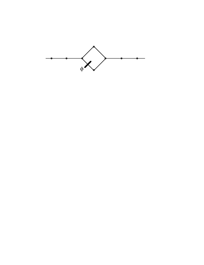
Figure 2. Graph for example

We can find the unnormalized eigenstates for this graph, and one set of them can be described as having an incoming wave from the left, an outgoing transmitted wave going to the right, and a reflected wave going to the left. A second set will have an incoming wave from the right, an outgoing trasmitted wave to the left, and a refelected wave to the right. The mathematical status of these objects will be explored in Sections 7 and 8. Finally, there may be bound states, i.e. eigenstates that are localized in the region between the two vertices with three edges. Now, let us denote the left three-edge vertex by $0$ and the right one by $2$, and number the vertices on the lines correspondingly, from $2$ to plus infinity to the right and from $0$ to minus infinity to the left. The eigenstates with a wave incident from the left take the form

(3.1) $$|\Psi\rangle = \sum_{j=-\infty}^{-1}(e^{ij\theta}|j,j+1\rangle+b_{-1}e^{-i(j+1)\theta}|j+1,j\rangle)+|\Psi_{02}\rangle$$

$$+\sum_{j=2}^{\infty}a_{2}e^{i(j-2)\theta}|j,j+1\rangle,$$

where $|\Psi_{02}\rangle$ is the part of the eigenfunction between vertices $0$ and $2$, and $e^{-i\theta}$ is the eigenvalue of the operator $U$ that advances the walk one step. The first term can be thought of as the incoming wave; it is confined to the region between negative infinity and $0$, and consists of states in which the particle is moving to the right. The term proportional to $b_{-1}$ is the reflected wave. It is also confined to the region between negative infinity and $0$, but consists of states in which the particle is moving to the left. Finally, the term proportional to $a_{2}$ is the transmitted, being confined to the region from $2$ to infinity, and consisting of states with the particle moving to the right. The coefficient $b_{-1}$ can be interpretted as the amplitude for the incoming wave to be reflected, and $a_{2}$ as the amplitude to be transmitted. Denoting the upper vertex between $0$ and $2$ as $1A$ and the lower one as $1B$, we can express $|\Psi_{02}\rangle$ as

(3.2) $$|\Psi_{02}\rangle = a_{0A}|0,1A\rangle+a_{1A}|1A,2\rangle+b_{0A}|1A,0\rangle+b_{1A}|2,1A\rangle$$

$$+a_{0B}|0,1B\rangle+a_{1B}|1B,2\rangle+b_{0B}|1B,0\rangle+b_{1B}|2,1B\rangle.$$

The solution of the equation $U|\Psi\rangle=e^{-i\theta}|\Psi\rangle$ is given in the appendix.

One can define a transmission coefficient for this graph, which is just the ratio of the intensities of the outgoing transmitted and the incoming waves,

(3.3) $$T=|a_{2}|^{2}=\left|\frac{4(1+e^{-i\phi})(1-e^{-i(4\theta+\phi)})}{e^{-4i\theta}(1+e^{-i\phi})^{2}-(3e^{-i(4\theta+\phi)}-1)^{2}}\right|^{2}.$$

One finds that for $\phi=0$, T is nonzero, because the two paths from $0$ to $2$ interfere constructively, while when $\phi=\pi$ they interfere destructively, which results in $T=0$. Therefore, the behavior of the walk strongly depends on the value of the phase shift.

4. Hitting times

Suppose we want to find out whether the particle making the walk is on the edge between vertices $j$ and $j+1$. The relevant projection operator is

(4.1) $$P_{j}=|j,j+1\rangle\langle j,j+1|+|j+1,j\rangle\langle j+1,j|.$$

If we obtain $1$ the particle is on that edge, and if we obtain $0$, it is not. What we wish to find out is, if the particle is initially in the state $|\Psi(0)\rangle$, the probability that the particle is not on the edge for the first $n$ steps of the walk, but is on the $(n+1)$st. We measure $P_{j}$ after every step, and we have to take the effect of these meaurements into account in describing the dynamics of the wave function.

Let us first see what happens after one step. Let $U$ be the unitary operator that advances the walk one step. The probability that the particle is not on the edge between $j$ and $j+1$ after one step, $p(1)$, is

(4.2) $$p(1)=\|(I-P_{j})U\Psi(0)\|^{2}.$$

and the quantum state, assuming the particle was not found on this edge, is

(4.3) $$|\Psi(1)\rangle=\frac{(I-P_{j})U|\Psi(0)\rangle}{\|(I-P_{j})U\Psi(0)\|}.$$

Now let us go one more step to see the pattern. The probability that the particle is not on the edge between $j$ and $j+1$ after either the first or second steps, $p(2)$, is

(4.4) $$p(2) = p(1)\|(I-P_{j})U\Psi(1)\|^{2}$$

$$= \|(I-P_{j})U(I-P_{j})U\Psi(0)\|^{2},$$

and the quantum state, assuming the particle was not found on the edge after either step, is

(4.5) $$|\Psi(2)\rangle=\frac{(I-P_{j})U|\Psi(1)\rangle}{\|(I-P_{j})U\Psi(1)\|}.$$

In general, if $p(n)$ is the probability of not finding the particle on the edge between $j$ and $j+1$ after each of $n$ steps, then

(4.6) $$p(n)=p(n-1)\|(I-P_{j})U\Psi(n-1)\|^{2},$$

where $|\Psi(n-1)\rangle$ is the quantum state after $n-1$ steps and $n-1$ measurements indicating that the particle was not on the designated edge. We also have that

(4.7) $$|\Psi(n)\rangle=\frac{(I-P_{j})U|\Psi(n-1)\rangle}{\|(I-P_{j})U\Psi(n-1)\|}.$$

Let us now proceed by induction. We shall assume that

$$p(n)=\|[(I-P_{j})U]^{n}\Psi(0)\|^{2}$$

(4.8) $$|\Psi(n)\rangle=\frac{[(I-P_{j})U]^{n}|\Psi(0)\rangle}{\|[(I-P_{j})U]^{n}\Psi(0)\|},$$

which clearly holds for $n=1,2$. Substitution of the second of these equations into Eq. (4.7) yields

(4.9) $$|\Psi(n+1)\rangle=\frac{(I-P_{j})U|\Psi(n)\rangle}{\|(I-P_{j})U\Psi(n)\|},$$

so that part of our induction hypothesis is verfied. From Eq. (4.6) we find that

(4.10) $$p(n+1) = \|[(I-P_{j})U]^{n}\Psi(0)\|^{2}\|(I-P_{j})U\Psi(n)\|^{2}$$

$$= \|[(I-P_{j})U]^{n+1}\Psi(0)\|^{2},$$

which proves the remaining part. This result is easily generalized to the case of making measurements to determine whether the particle is on a set of edges instead of on a single edge. A similar result for the coined quantum walk was derived by Bach, et al. [11].

The hitting time for a random walk on a graph is the expected number of steps in a walk that starts at one specified vertex and stops on first reaching a second specified vertex. In order to calculate this we need the probability that a walk starting on the first vertex does not reach the second for its first $n-1$ steps, but does reach it on the $n$th step. The corresponding quantity for a quantum walk, which we shall call $q(n)$, is the probability that a walk starting in the state $|\Psi(0)\rangle$ is not measured to be on the edge between $j$ and $j+1$ for the first $n-1$ steps, but is measured to be on that edge at the $n$th step. This probability is given by

(4.11) $$q(n) = p(n-1)\|P_{j}U\Psi(n-1)\|^{2}$$

$$= \|P_{j}U[(I-P_{j})U]^{n-1}\Psi(0)\|^{2}.$$

The particle making this walk may never be found to be on the edge between $j$ and $j+1$ at all, and the probability that it is, is given by

(4.12) $$P_{out}=\sum_{n=1}^{\infty}q_{n}.$$

We can define a conditional hitting time for this walk, $h$, as

(4.13) $$h=\frac{1}{P_{out}}\sum_{n=1}^{\infty}nq_{n}.$$

This quantity provides an an indication of how many steps a walk that does reach the edge between $j$ and $j+1$ will require.

Let us now consider the situation depicted in Figure 3. We start the walk on the edge $|-1,0\rangle$ moving to the right, and we are interested in how long it takes to get to the edge $|j,j+1\rangle$, where $G$ is a general graph with a finite number of edges and vertices. The vertices outside of the graph, $G$, for example, $-1$ and $j+1$, have a transmission amplitude, $t=1$. We shall denote the entire graph, $G$ plus the tails, as $\tilde{G}$. The case considered in the previous section is a special case of this situation. When calculating the probability, $q(n)$, that the walk arrives at the edge $|j,j+1\rangle$ for the first time after $n$ steps, we need to evaluate (see Eq. (4.11))

(4.14) $$P_{j}U[(I-P_{j})U]^{n-1}=P_{j}U^{n}-\sum_{k=1}^{n-1}P_{j}U^{(n-k)}P_{j}U^{k}+\ldots$$

We first note that once the particle leaves the graph, $G$, it moves one unit to the right with each step. That means that terms of the form $P_{j}U^{m}P_{j}U^{k}|-1,0\rangle$, for $m>0$, are zero, because the first $P_{j}$ puts the particle in the state $|j,j+1\rangle$, and the operator $U^{m}$ moves it $m$ steps to the right, so that the particle in now in the state $|j+m,j+m+1\rangle$. The projection $P_{j}$ acting on this state gives zero. Therefore, only the first term on the right-hand side of Eq. (4.14) gives a nonzero contribution. That means that in this case, we have

(4.15) $$q(n)=\langle\Psi(0)|(U^{\dagger})^{n}P_{j}U^{n}|\Psi(0)\rangle.$$

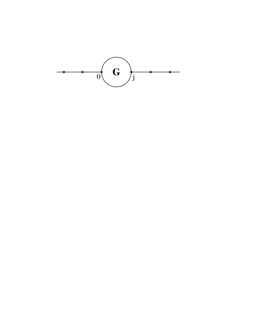
Figure 3. A general graph, $G$, with tails attached to two if its vertices

We now want to relate the probability $q(n)$ to the transmission coefficient of the graph, which we shall define shortly. The eigenstates of the system can be grouped into three sets, those with the particle coming in from the left, those with the particle coming in from the right, and bound states. The eigenstates of this system corresponding to the particle coming in from the left are

(4.16) $$|\Psi_{l}(\theta)\rangle = \sum_{k=-\infty}^{-1}(e^{i(k+1)\theta}|k,k+1\rangle+r(\theta)e^{-i(k+1)\theta}|k+1,k\rangle)+|\Psi_{G}(\theta)\rangle$$

$$+\sum_{k=j}^{\infty}t(\theta)e^{i(k-j)\theta}|k,k+1\rangle,$$

where $r(\theta)$ is the reflection coefficient, $t(\theta)$ is the transmission coefficient, and $|\Psi_{G}(\theta)\rangle$ is the part of the eigenfunction inside the graph $G$. This state is, in fact, not in $L^{2}(E)$, and its mathematical significance will be clarified in a later section. In Appendix B we show that

(4.17) $$|r(\theta)|^{2}+|t(\theta)|^{2}=1.$$

For the initial state of our walk we will choose $|-1,0\rangle$, and we want to express this state in terms of the eigenstates in Eq. (4.16). To do so we integrate $|\Psi_{l}(\theta)\rangle$ from $0$ to $2\pi$, finding

(4.18) $$\frac{1}{2\pi}\int_{0}^{2\pi}d\theta|\Psi_{l}(\theta)\rangle = |-1,0\rangle+\frac{1}{2\pi}\int_{0}^{2\pi}d\theta[\sum_{k=-\infty}^{-1}r(\theta)e^{-i(k+1)\theta}|k+1,k\rangle]$$

$$+\frac{1}{2\pi}\int_{0}^{2\pi}d\theta[|\Psi_{G}(\theta)\rangle+\sum_{k=j}^{\infty}t(\theta)e^{i(k-j)\theta}|k,k+1\rangle].$$

By setting $z=\exp(i\theta)$ the integrals on the right-hand side of the above equation can be turned into integrals along the unit circle, which we shall denote by $C$, in the complex plane. These integrals are of the form

$$\int_{C}dz\,z^{m-1}r(z) \int_{C}dz\,\frac{1}{z}|\Psi_{G}(z)\rangle$$

(4.19) $$\int_{C}dz\,z^{m-1}t(z)$$ ,

where $m\geq 0$. As we shall show in Section 7, $r(z)$, $t(z)$, and $|\Psi_{G}(z)\rangle$ are analytic functions of $z$ on the unit circle and in its interior, and they all vanish when $z=0$. This implies that all of the above integrals are zero. Therefore, we can conclude that

(4.20) $$|-1,0\rangle=\frac{1}{2\pi}\int_{0}^{2\pi}d\theta|\Psi_{l}(\theta)\rangle.$$

Now we have that

(4.21) $$q(n)=|\langle j,j+1|U^{n}|-1,0\rangle|^{2},$$

and

(4.22) $$\langle j,j+1|U^{n}|-1,0\rangle = \frac{1}{2\pi}\int_{0}^{2\pi}d\theta e^{-in\theta}\langle j,j+1|\Psi_{l}(\theta)\rangle$$

$$= \frac{1}{2\pi}\int_{0}^{2\pi}d\theta e^{-in\theta}t(\theta).$$

Therefore, we find

(4.23) $$q(n)=\left|\frac{1}{2\pi}\int_{0}^{2\pi}d\theta e^{-in\theta}t(\theta)\right|^{2},$$

which relates a walk probability, the probability to land on the edge between $j$ and $j+1$ for the first time after $n$ steps, to the S matrix of the graph $G$.

We can rewrite the integral appearing in the above expression for $q(n)$ as a contour integral over the unit circle, $C$ by setting $z=e^{i\theta}$. This gives us

(4.24) $$\frac{1}{2\pi}\int_{0}^{2\pi}d\theta e^{-in\theta}t(\theta)=\frac{1}{2\pi i}\int_{C}dz\frac{1}{z^{n+1}}t(z).$$

Because, as we shall see, $t(z)$ is analytic in a region containing the unit circle and its interior, the only contribution to the integral in Eq. (4.24) comes from the pole at the origin that is due to the $1/z^{n+1}$ factor. This fact makes it straightforward to evaluate the above integral, by just finding the residue of the pole at the origin, giving us

(4.25) $$\frac{1}{2\pi i}\int_{C}dz\frac{1}{z^{n+1}}t(z)=\left.\frac{1}{n!}\frac{d^{n}}{dz^{n}}t(z)\right|_{z=0}.$$

This is just the $n^{\rm th}$ coefficient in the Taylor expansion of $t(z)$ about the origin, i.e. if

(4.26) $$t(z)=\sum_{n=0}^{\infty}c_{n}z^{n},$$

then we have that $q(n)=|c_{n}|^{2}$. The conditional hitting time, defined in Eq. (4.13), is then given by

(4.27) $$h=\frac{1}{P_{out}}\sum_{n=0}^{\infty}n|c_{n}|^{2}\hskip 28.45274ptP_{out}=\sum_{n=0}^{\infty}|c_{n}|^{2}.$$

We now note that

(4.28) $$t^{\ast}(z)z\frac{dt}{dz}=\sum_{m=0}^{\infty}\sum_{n=1}^{\infty}nc^{\ast}_{m}c_{n}(z^{\ast})^{m}z^{n},$$

from which it follows, setting $z=\exp(i\theta)$ and integrating, that

(4.29) $$h=\frac{1}{2\pi P_{out}}\int_{0}^{2\pi}d\theta t^{\ast}(e^{i\theta})e^{i\theta}\left.\frac{dt}{dz}\right|_{z=e^{i\theta}}.$$

Similarly, we have that

(4.30) $$P_{out}=\frac{1}{2\pi}\int_{0}^{2\pi}d\theta\,|t(e^{i\theta})|^{2}.$$

The integrals in the previous two equations can also be expressed as contour integrals if we define the “reflected” transmission amplitude, $t_{R}(z)$ to be $t_{R}(z)=t(z^{\ast})^{\ast}$. We then have that

$$P_{out}=\frac{1}{2\pi i}\int_{C}dz\left(\frac{1}{z}\right)t_{R}\left(\frac{1}{z}\right)t(z)$$

(4.31) $$h=\frac{1}{2\pi iP_{out}}\int_{C}dzt_{R}\left(\frac{1}{z}\right)\frac{dt(z)}{dz}.$$

Thus, we see that both the probability of first hitting the edge between $j$ and $j+1$ in $n$ steps and the hitting time to reach this edge are related to the transmission amplitude of the graph.

5. Application to example

Let us now apply this formula to a walk on the graph discussed in Section 3. The transmission amplitude for this graph is

(5.1) $$t(\theta)=\frac{4e^{-i\theta}(1+e^{-i\phi})(1-e^{-i(4\theta+\phi)})}{e^{-4i\theta}(1+e^{-i\phi})^{2}-(3e^{-i(4\theta+\phi)}-1)^{2}}.$$

and

(5.2) $$t(z)=\frac{4z^{3}(1+e^{-i\phi})(z^{4}-e^{-i\phi})}{z^{4}(1+e^{-i\phi})^{2}-(3e^{-i\phi}-z^{4})^{2}}.$$

From this expression we see explicitly that $t(z)$ is analytic inside and on the unit circle.

Considering the case $\phi=0$ we find the simple expression

(5.3) $$t(z)=\frac{8z^{3}}{9-z^{4}}.$$

Inserting this result into the expressions in the previous section, it is straightforward to perform the integrations, and we find that

(5.6) $$q(n) = \left\{\begin{array}[]{cr}\left(\frac{8}{9^{(n+1)/4}}\right)^{2}&{\rm if}\ n=3\ {\rm mod}4\\ 0&{\rm otherwise}\end{array}\right.$$

(5.7) $$P_{out} = \frac{4}{5}.$$

For small $n$, it is relatively straightforward to verify the expression for $q(n)$ by adding up the amplitudes for the possible paths from $|-1,0\rangle$ to $|2,3\rangle$ of length $n$.

Another issue that deserves mention is the existence of bound states. In standard quantum scattering theory, if a potential has bound states, these are orthgonal to all scattering states. What we mean by a bound state of a graph, is an eigenstate of $U$ whose support is confined to $G$. If our graph has bound states, then these states could not be accessed by a particle coming in from one of the tails, e.g. from the left. This follows from the fact that the initial state is orthogonal to any bound state (a state localized on one of the tails is automatically orthogonal to one that is localized in $G$), and if $\Psi_{init}$ is the initial state, and $\Psi_{bnd}$ is the localized eigenstate with eigenvalue $\exp(-i\theta_{b})$, we have

(5.8) $$\langle\Psi_{bnd}|U^{n}\Psi_{init}\rangle=e^{-in\theta_{b}}\langle\Psi_{bnd}|\Psi_{init}\rangle=0.$$

This limits the walks that particles with initial states of this type can perform, because, as the above equation shows, the state of the walk at any time must be orthogonal to all of the bound states.

In order to find the bound states in our example we consider a state $|\Psi\rangle$ that is located on the four edges connecting the vertices $0$, $1A$, $1B$, and $2$, i.e.

(5.9) $$|\Psi\rangle = a_{0A}|0,1A\rangle+a_{1A}|1A,2\rangle+b_{0A}|1A,0\rangle+b_{1A}|2,1A\rangle$$

$$+a_{0B}|0,1B\rangle+a_{1B}|1B,2\rangle+b_{0B}|1B,0\rangle+b_{1B}|2,1B\rangle.$$

We then solve the equation $U|\Psi\rangle=e^{-i\theta}|\Psi\rangle$. This equation only has a solution when $\phi=0$, and in that case the eigenvalues are $i^{m}$, where $m=0,\ldots 3$. The eigenstates in this case are given by

$$a_{0A}=\frac{1}{2\sqrt{2}} b_{0A}=-\frac{i^{m}}{2\sqrt{2}}$$

$$a_{1A}=\frac{1}{2i^{m}\sqrt{2}} b_{1A}=\frac{-(-1)^{m}}{2\sqrt{2}}$$

$$a_{0B}=\frac{-1}{2\sqrt{2}} b_{0B}=\frac{i^{m}}{2\sqrt{2}}$$

(5.10) $$a_{1B}=\frac{-1}{2i^{m}\sqrt{2}} b_{1B}=\frac{(-1)^{m}}{2\sqrt{2}}$$

A simple basis for the space spanned by these eigenstates is

$$|u_{1}\rangle = \frac{1}{\sqrt{2}}(|0,1A\rangle-|0,1B\rangle)$$

$$|u_{2}\rangle = \frac{1}{\sqrt{2}}(|1A,2\rangle-|1B,2\rangle)$$

$$|u_{3}\rangle = \frac{1}{\sqrt{2}}(|1B,0\rangle-|1A,0\rangle)$$

(5.11) $$|u_{4}\rangle = \frac{1}{\sqrt{2}}(|2,1B\rangle-|2,1A\rangle).$$

A state resulting from a walk starting on the tails, will be orthogonal to the subspace spanned by these four states. A walk starting in this subspace will never leave the subspace, and hence, will never escape into the tails.

For all of the eigenvalues except those given by $i^{m}$, the corresponding space of (unnormalized) eigenvectors is two dimensional. It is spanned by two scattering states, one with a incoming wave from the left, and one with an incoming wave from the right. These states are orthogonal. At the eigenvalues $i^{m}$ the space of eigenvectors becomes three dimensional. In addition to the two scattering states, there is one bound state. All of these state are mutually orthogonal.

6. Time reversal

In quantum one-dimensional scattering problems, the time reversal invariance of the Hamiltonian is used to prove that the transmission amplitude for a wave coming from the left is the same as that for a wave coming from the right. Here we would like to see if something similar is possible for quantum walks.

Our first task is to define a time-reversal operator. The standard time-reversal operator is anti-unitary, does not affect positions, and reverses velocities. This suggests that we define the anti-unitary operator, $\hat{T}$, where the hat is used to indicate that the operator is anti-linear, by

(6.1) $$\hat{T}|A,B\rangle=|B,A\rangle.$$

Note that $\hat{T}$ is its own inverse. For a walk to be time-reversal invariant, we want the operator that advances the walk one step, $U$, to be taken into its inverse when conjugated by $\hat{T}$,

(6.2) $$\hat{T}U\hat{T}=U^{-1}=U^{\dagger},$$

that is, conjugation with $\hat{T}$ changes the operator that moves the walk forward one step into the one that moves it backwards one step.

Let us see what this condition implies about $U$. Let $k$ enumerate the vertices that are connected to $A$ by an edge (one of which is $B$). This set will be denoted by $\Gamma(A)$. We find that

$$\hat{T}U\hat{T}|A,B\rangle = \sum_{k}\langle A,k|U|B,A\rangle^{\ast}|k,A\rangle$$

(6.3) $$U^{-1}|A,B\rangle = \sum_{k}\langle A,B|U|k,A\rangle^{\ast}|k,A\rangle$$

These will be the same if

(6.4) $$\langle A,k|U|B,A\rangle=\langle A,B|U|k,A\rangle,$$

so that $U$ will satisfy the condition of time-reversal invariance if for all vertices $A$, and $k,k^{\prime}\in\Gamma(A)$, we have

(6.5) $$\langle A,k|U|k^{\prime},A\rangle=\langle A,k^{\prime}|U|k,A\rangle.$$

We find that equal-transmission vertices satisfy this condition, and they still satisfy it if phase shifters are put into the edges. We shall henceforth confine our attention to graphs that do satisfy this condition.

If $|\Psi\rangle$ is an eigenstate of $U$ with eigenvalue $\exp(-i\theta)$, and $U$ is time-reversal invariant, then

$$\hat{T}U\hat{T}|\Psi\rangle = e^{i\theta}|\Psi\rangle$$

(6.6) $$U\hat{T}|\Psi\rangle = e^{-i\theta}\hat{T}|\Psi\rangle,$$

where we have made use of Eq. (6.2). This implies that if $|\Psi\rangle$ is an eigenstate of $U$, then so is $\hat{T}|\Psi\rangle$, with the same eigenvalue. Note that if $|\Psi\rangle$ is a bound state, this equation implies either that $|\Psi\rangle$ is invariant under the action of $\hat{T}$, or that the eigenvalue $\exp(-i\theta)$ is degenerate.

We can now show that the transmission coefficients from both directions are equal. Consider two eigenstates, each with eigenvalue $\exp(-i\theta)$, one incident from the left, and one incident from the right

$$|\Psi_{l}(\theta)\rangle = \sum_{k=-\infty}^{-1}(e^{i(k+1)\theta}|k,k+1\rangle+r_{l}(\theta)e^{-i(k+1)\theta}|k+1,k\rangle)+|\Psi_{Gl}(\theta)\rangle$$

$$+\sum_{k=j}^{\infty}t_{l}(\theta)e^{i(k-j)\theta}|k,k+1\rangle$$

(6.7) $$|\Psi_{r}(\theta)\rangle = \sum_{k=-\infty}^{-1}t_{r}(\theta)e^{-i(k+1)\theta}|k+1,k\rangle+|\Psi_{Gr}\rangle$$

$$\sum_{k=j}^{\infty}(e^{-i(k-j)\theta}|k+1,k\rangle+r_{r}(\theta)e^{i(k-j)\theta}|k,k+1\rangle).$$

Now, consider the eigenstate

(6.8) $$|\Psi\rangle=A|\Psi_{l}\rangle+B|\Psi_{r}\rangle.$$

If we apply $\hat{T}$ to this state, we must obtain an eigenstate of $U$ with an eigenvalue of $\exp(-i\theta)$, which must, therefore, be a linear combination of $|\Psi_{l}\rangle$ and $|\Psi_{r}\rangle$,

(6.9) $$\hat{T}|\Psi\rangle=C|\Psi_{l}\rangle+D|\Psi_{r}\rangle.$$

This implies that

$$A^{\ast}=Cr_{l}+Dt_{r} A^{\ast}t^{\ast}_{l}+B^{\ast}r^{\ast}_{r}=D$$

(6.10) $$A^{\ast}r^{\ast}_{l}+B^{\ast}t^{\ast}_{r}=C B^{\ast}=Ct_{l}+Dr_{r}.$$

Substituting from the second and third of these equations into the first, gives us

(6.11) $$|r_{l}|^{2}+t_{r}t^{\ast}_{l}=1\hskip 28.45274ptr_{l}t^{\ast}_{r}+t_{r}r^{\ast}_{r}=0.$$

The first of these equations, and the fact that $|r_{l}|^{2}+|t_{l}|^{2}=1$, gives us that $t_{r}=t_{l}$. Therefore, time-reversal invariance does imply that the left and right transmission amplitudes are the same.

7. Analyticity of the reflection and transmission amplitudes

We now want to see how to find, schematically, the reflection and transmission amplitudes of a general graph, and then deduce some of their properties. In particular we want to show that they are analytic in a region that contains the unit circle and its interior.

We begin by considering the graph $\tilde{G}$ and denote the set of oriented edges of $\tilde{G}$ by $E$. The space in which the walk takes place is $\mathcal{H}=L^{2}(E)$, and this immediately presents us with a problem, because $|\Psi_{l}(\theta)\rangle$ (see Eq. (4.16)), through which the reflection and transmission amplitudes are defined, is not in $L^{2}(E)$. It can certainly be viewed as a complex-valued function on the set $E$, $(A,B)\in E\rightarrow\langle A,B|\Psi_{l}(\theta)\rangle$, and it is in this sense that we take the following calculations until we have more information on the nature of the specific functions.

The transmission and reflection amplitudes are found by solving the eigenvalue equation,

(7.1) $$U|\Psi\rangle=\exp(-i\theta)|\Psi\rangle.$$

A direct calculation shows that this is equivalent to

(7.2) $$U(|-1,0\rangle+|\Psi_{G}(\theta)\rangle)=e^{-i\theta}(|\Psi_{G}(\theta)\rangle+r(\theta)|0,-1\rangle+t(\theta)|j,j+1\rangle).$$

Now let $\mathcal{H}_{G}$ be the subspace of $\mathcal{H}$ spanned by the oriented edges of $G$, $\mathcal{H}_{3}$ be the subspace of $\mathcal{H}$ spanned by the oriented edges $\{|-1,0\rangle,|0,-1\rangle,|j.j+1\rangle\}$, $P_{G}$ be the orthogonal projection onto the space $\mathcal{H}_{G}$, and $P_{3}$ be the orthogonal projection onto the space $\mathcal{H}_{3}$. In addition, define $\tilde{\mathcal{H}}=\mathcal{H}_{3}\oplus\mathcal{H}_{G}$ and $\tilde{P}$ as the orthogonal projection onto $\tilde{\mathcal{H}}$. We can view the elements of $\tilde{\mathcal{H}}$ as column vectors of complex numbers

$$\mathbf{v}=\left(\begin{array}[]{c}v_{1}\\ v_{2}\\ v_{3}\\ \mathbf{v}_{G}\end{array}\right),$$

where $v_{1}$ is the coefficient of $|-1,0\rangle$, $v_{2}$ is the coefficient of $|0,-1\rangle$, $v_{3}$ the coefficient of $|j,j+1\rangle$ and $\mathbf{v}_{G}$ the $2N$-tuple of coefficients of the edges of $G$ (we assume that $G$ has $N$ edges). In this notation, Eq. (7.2) becomes

(7.3) $$e^{-i\theta}\left(\begin{array}[]{c}0\\ r(\theta)\\ t(\theta)\\ \mathbf{v}_{G}\end{array}\right)=\left(\begin{array}[]{cc}\mathbf{X}&\mathbf{Y}\\ \mathbf{W}&\mathbf{G}\end{array}\right)\left(\begin{array}[]{c}1\\ 0\\ 0\\ \mathbf{v}_{G}\end{array}\right).$$

where

(7.4) $$\left(\begin{array}[]{cc}\mathbf{X}&\mathbf{Y}\\ \mathbf{W}&\mathbf{G}\end{array}\right)=(\tilde{P}U\tilde{P})=\left(\begin{array}[]{cc}P_{3}UP_{3}&P_{3}UP_{G}\\ P_{G}UP_{3}&P_{G}UP_{G}\end{array}\right).$$

In the above equation, $X$ is a $3\times 3$ matrix, $Y$ is a $2N\times 3$ matrix, $W$ is a $3\times 2N$ matrix, and $G$ is a $2N\times 2N$ matrix. The second and third columns of both $\mathbf{X}$ and $\mathbf{W}$ are identically zero. We also note that the first rows of both $X$ and $Y$ are identically zero.

It is possible to break the solution of Eq. (7.3) into two parts. Denote the single nonzero column of $\mathbf{W}$ (the first one) by $\mathbf{w}$, i.e.

(7.5) $$\mathbf{w}=\mathbf{W}\left(\begin{array}[]{c}1\\ 0\\ 0\\ \mathbf{0}\end{array}\right),$$

where $\mathbf{0}$ is a $2N$-tuple of zeroes, so that $\mathbf{w}\in\mathcal{H}_{G}$. The first step in solving Eq. (7.3) is solving the equation in $\mathcal{H}_{G}$,

(7.6) $$(e^{-i\theta}\mathbf{I}-\mathbf{G})\mathbf{v}_{G}=\mathbf{w},$$

where $\mathbf{I}$ is the $2N\times 2N$ identity matrix. Once we have found $\mathbf{v}_{G}$ from this equation, we insert the solution into Eq. (7.3) in order to find $r(\theta)$ and $t(\theta)$.

We can extend the reflection and transmission amplitudes into the complex plane by replacing $\exp(-i\theta)$ in the above equations by $1/z$. This will yield the functions $t(z)$ and $r(z)$. In particular we have that if $\mathbf{v}_{G}(z)$ is a solution to

(7.7) $$(\mathbf{I}-z\mathbf{G})\mathbf{v}_{G}=z\mathbf{w},$$

then

$$t(z) = \sum_{(k,l)\in G}zY_{(j,j+1);(k,l)}v_{G;(k,l)}(z)$$

(7.8) $$r(z) = z[X_{(0,-1);(-1,0)}+\sum_{(k,l)\in G}Y_{(0,-1);(k,l)}v_{G;(k,l)}(z)],$$

where the sums are over all edges in $G$.

We are first interested in determining whether $t(z)$ is analytic inside the unit circle. This will be the case if Eq. (7.6) can be solved for all $|z|<1$, which will be true if the matrix $\mathbf{I}-z\mathbf{G}$ is invertible for $|z|<1$. This follows from the result that if an operator, $T(z)$, is analytic in some region of the complex plane, so is its inverse, $T^{-1}(z)$ provided it exists [29]. Because $\mathbf{G}=P_{G}UP_{G}$ we have that $\|\mathbf{G}\|\leq 1$, which implies that if $|z|<1$, then $\mathbf{I}-z\mathbf{G}$ is invertible.

We now have that $t(z)$ and $r(z)$ are analytic inside the unit circle, but what about on the circle itself and a bit beyond? To show that they are, we need to refine our arguments.

Lemma 7.1.

1. $(e^{-i\theta}I-P_{G}UP_{G})|u\rangle=0$ if and only if $|u\rangle$ is an $L^{2}$ eigenstate of $U$ with support in the edges of $G$. We call these bound states.

2. If $|w\rangle=P_{G}|-1,0\rangle$, then $\langle u|w\rangle=0$, where $|u\rangle$ is any bound state.

Proof.

1. (7.9) $$0 = (e^{-i\theta}I-P_{G}UP_{G})|u\rangle$$

   $$= e^{-i\theta}P_{G}^{\perp}|u\rangle+e^{-i\theta}P_{G}|u\rangle-P_{G}UP_{G}|u\rangle,$$

   so $P_{G}^{\perp}|u\rangle=0$ and the support of $|u\rangle$ lies in the edges of $G$. Therefore, $P_{G}U|u\rangle=\exp(-i\theta)|u\rangle$, which implies that $P_{G}U|u\rangle=U|u\rangle$, and $|u\rangle$ is the desired eigenstate.

2. This follows from

   (7.10) $$\langle u|w\rangle=\langle u|P_{G}U|-1,0\rangle=\langle U^{\dagger}u|-1,0\rangle=0.$$

∎

If $e^{-i\theta}$ corresponds to a bound state, then the operator $(e^{-i\theta}\mathbf{I}-\mathbf{G})$ is not invertible. At the moment this leaves us without a method of defining $t(z)$ and $r(z)$ for values of $z$ corresponding to bound states. We would like to show, however, that for these values of $z$, scattering solutions, that is solutions to Eq. (7.6), also exist. These solutions can then be used to define $t(z)$ and $r(z)$.

Let $|u_{1}\rangle,\ldots|u_{K}\rangle$ be the eigenstates of $U$, where $|u_{k}\rangle\in\mathcal{H}_{G}$ and $U|u_{k}\rangle=\exp(-i\theta_{k})|u_{k}\rangle$. Let $\mathcal{H}_{b}$ be the span of $\{|u_{1}\rangle,\ldots|u_{K}\rangle\}$. $\mathcal{H}_{b}$ is an invariant subspace of both $U$ and $\mathbf{G}$. Let $\mathcal{H}_{1}=\mathcal{H}_{b}^{\perp}$ as a subspace of $\mathcal{H}_{G}$, and let $P_{1}$ be the orthogonal projection of $\mathcal{H}_{G}$ onto $\mathcal{H}_{1}$, and $\mathbf{G}_{1}=P_{1}\mathbf{G}P_{1}$. We wish to solve the equation

(7.11) $$(\mathbf{I}_{\mathcal{H}_{1}}-z\mathbf{G}_{1})\mathbf{v}=z\mathbf{w},$$

on $\mathcal{H}_{1}$. Because of the construction of $\mathcal{H}_{1}$, we are guaranteed that there exists an $\epsilon>0$ such that $(\mathbf{I}_{\mathcal{H}_{1}}-z\mathbf{G}_{1})$ is invertible on $\mathcal{H}_{1}$ for $|z|<1+\epsilon$. This allows us to define

$$|\Psi_{G}(z)\rangle = \mathbf{v}_{G}(z)=(\mathbf{I}_{\mathcal{H}_{1}}-z\mathbf{G}_{1})^{-1}z\mathbf{w}$$

$$r(z) = z(\langle 0,-1|U|-1,0\rangle+\langle 0,-1|U|\Psi_{G}(z)\rangle)$$

(7.12) $$t(z) = z(\langle j,j+1|U|-1,0\rangle+\langle j,j+1|U|\Psi_{G}(z)\rangle),$$

and

(7.13) $$|\Psi(z)\rangle = \sum_{k=-\infty}^{-1}z^{(k+1)}|k,k+1\rangle+\sum_{k=-\infty}^{-1}r(z)z^{-(k+1)}|k+1,k\rangle$$

$$+|\Psi_{G}(z)\rangle+\sum_{k=j}^{\infty}t(z)z^{k-j}|k,k+1\rangle.$$

We shall summarize our results in a theorem.

Theorem 7.2.

1. The complex-valued functions $r(z)$ and $t(z)$, and the function $|\Psi_{G}(z)\rangle$, which takes values in $\mathcal{H}_{1}$, are analytic functions on the disc $|z|<1+\epsilon$.

2. For each $z\in D=\{z|0<|z|<1+\epsilon\}$, the punctured disc, $|\Psi(z)\rangle$ is an element of $L^{\infty}(E)$, and $|\Psi(z)\rangle$ is an analytic function of $z$ on the domain $D$ with values in $L^{\infty}(E)$.

3. $|\Psi(z)\rangle$ is the solution to the generalized eigenvalue equation $zU|\Psi(z)\rangle=|\Psi(z)\rangle$.

Let us now make two brief observations. First, note that the functions $t(\theta)$ and $r(\theta)$ are just the restrictions of $t(z)$ and $r(z)$ to the unit circle. Second, we see that the above theorem, along with the expressions for $t(z)$ and $r(z)$, provides the necessary conditions for all of the integrals in Eq. (4) to vanish.

8. Spectral results

The formal eigenvectors $|\Psi(\theta)\rangle$, which we just constructed, are elements of $L^{\infty}(E)$, and hence, for any $|v\rangle\in L^{1}(E)$, the inner product $\langle\Psi(\theta)|v\rangle$ is well-defined, because it is absolutely summable. However, if $|v\rangle$ is merely in $L^{2}(E)$, $\langle\Psi(\theta)|v\rangle$ is not necessarily summable. Due to the specific form of $|\Psi(\theta)\rangle$, this sum represents a Fourier series with square-summable coefficients, and hence it is a function in $L^{2}(T)$, where $T$ is the unit circle with the usual measure $d\theta$. We shall now exploit these two interpretations of our formulas.

Recall that $\mathcal{H}_{b}$ is the space of bound states, i.e. $L^{2}$ eigenfunctions of $U$. $\mathcal{H}_{b}$ is a finite-dimensional, $U$-invariant subspace of $\mathcal{H}$. Each element of $\mathcal{H}_{b}$ has its support contained among the edges of $G$. The function (vector) $|\Psi(\theta)\rangle$ constructed in the last section is seen to be the unique element of $L^{\infty}(E)$ such that,

1. $U|\Psi(\theta)\rangle=e^{-i\theta}|\Psi(\theta)\rangle$,

2. $\langle\Psi(\theta)|-1,0\rangle=1$,

3. $\langle\Psi(\theta)|v\rangle=0$ for any $|v\rangle\in\mathcal{H}_{b}$.

The analytic extension of $|\Psi(\theta)\rangle$ to $D=\{z|0<|z|<1+\epsilon\}$ is given by $|\Psi(z)\rangle$ (see Eq. (7.13)), and a direct application of the Cauchy integral theorem to $|\Psi(z)\rangle$ implies that

(8.1) $$\frac{1}{2\pi}\int_{0}^{2\pi}d\theta\,|\Psi(\theta)\rangle=|-1,0\rangle.$$

If $|v\rangle\in L^{1}$, then $\langle\Psi(\theta)|v\rangle$ is a continuous function on the circle, and

(8.2) $$\frac{1}{2\pi}\int_{0}^{2\pi}d\theta\,|\Psi(\theta)\rangle\langle\Psi(\theta)|v\rangle\in L^{\infty}(E).$$

In particular, if $|v\rangle=|-1,0\rangle$, we have

(8.3) $$|-1,0\rangle=\frac{1}{2\pi}\int_{0}^{2\pi}d\theta\,|\Psi(\theta)\rangle\langle\Psi(\theta)|-1,0\rangle.$$

From this we have that

(8.4) $$U^{k}|-1,0\rangle = \frac{1}{2\pi}\int_{0}^{2\pi}d\theta\,e^{-ik\theta}|\Psi(\theta)\rangle\langle\Psi(\theta)|-1,0\rangle$$

$$= \frac{1}{2\pi}\int_{0}^{2\pi}d\theta\,|\Psi(\theta)\rangle\langle(U^{\dagger})^{k}\Psi(\theta)|-1,0\rangle$$

$$= \frac{1}{2\pi}\int_{0}^{2\pi}d\theta\,|\Psi(\theta)\rangle\langle\Psi(\theta)|U^{k}|-1,0\rangle.$$

Hence, for each $|v\rangle$ in the linear span of the states $U^{k}|-1,0\rangle$, where $k$ is an integer, and for any trigometric polynomial $f$, we have the $L^{\infty}$ formulas

(8.5) $$|v\rangle = \frac{1}{2\pi}\int_{0}^{2\pi}d\theta\,|\Psi(\theta)\rangle\langle\Psi(\theta)|v\rangle$$

(8.6) $$f(U)|v\rangle = \frac{1}{2\pi}\int_{0}^{2\pi}d\theta\,f(e^{-i\theta})|\Psi(\theta)\rangle\langle\Psi(\theta)|v\rangle$$

(8.7) $$\langle v|f(U)|v\rangle = \frac{1}{2\pi}\int_{0}^{2\pi}d\theta\,f(e^{-i\theta})|\langle\Psi(\theta)|v\rangle|^{2}.$$

Eq. (8.6) is an $L^{\infty}$ formula, however, Eq. (8.7) is more general. It holds for any $|v\rangle$ that is a finite linear combination of the $U^{k}|-1,0\rangle$, for $k$ an integer. However, $\theta\rightarrow\langle\Psi(\theta)|v\rangle$ is an $L^{2}$ function on the circle for each $|v\rangle\in L^{2}(E)$. Let $\mathcal{H}_{L}$ be the closure of the linear span of the $U^{k}|-1,0\rangle$ in $\mathcal{H}=L^{2}(E)$. $\mathcal{H}_{L}$ is a closed $U$-invariant subspace of $\mathcal{H}$, and we see that Eq. (8.7) holds for $|v\rangle\in\mathcal{H}_{L}$ and for any complex-valued continuous function on $T$. Thus, by the Riesz-Markov theorem there exists a unique measure $\mu_{v}$, a Borel measure on the circle, called the spectral measure associated to $|v\rangle$, such that

(8.8) $$\langle v|f(U)|v\rangle=\int_{0}^{2\pi}d\mu_{v}(\theta)f(e^{-i\theta}),$$

and hence,

(8.9) $$d\mu_{v}=\frac{\langle v|\Psi(\theta)\rangle|^{2}}{2\pi}d\theta.$$

If we define $V_{L}:\mathcal{H}_{L}\rightarrow L^{2}(T)$ by

(8.10) $$V_{L}|v\rangle=\frac{1}{\sqrt{2\pi}}\langle\Psi(\theta)|v\rangle,$$

then Eq. (8.7) implies that $\|v\|=\|V_{L}v\|$, so that $V_{L}$ is an isometry from $\mathcal{H}_{L}$ to $L^{2}(T)$, and $V_{L}(\mathcal{H}_{L})$ is a closed subspace of $L^{2}(T)$. Finally, we have

(8.11) $$(V_{L}UV_{L}^{-1})g(\theta)=e^{-i\theta}g(\theta),$$

for $g\in V_{L}(\mathcal{H}_{L})$ which implies that $V_{L}(\mathcal{H}_{L})$ is an invariant subspace of the multiplication operator $g(\theta)\rightarrow\exp(-i\theta)g(\theta)$. Therefore, we have that $V_{L}(\mathcal{H}_{L})=L^{2}(T)$, and hence $V_{L}$ is a unitary operator of $\mathcal{H}_{L}$ onto $L^{2}(T)$. We can summarize our results to date in the following theorem.

Theorem 8.1.

Let $\mathcal{H}_{L}$ be the closed, linear, U-invariant subspace of $\mathcal{H}=L^{2}(E)$ generated by the states $U^{k}|-1,0\rangle$, for $k$ an integer. Let $|\Psi(\theta)\rangle$ be the generalized eigenfunctions constructed in the previous section, then for each $|v\rangle\in\mathcal{H}_{L}$,

(8.12) $$V_{L}|v\rangle=\frac{1}{\sqrt{2\pi}}\langle\Psi(\theta)|v\rangle,$$

defines a unitary operator from $\mathcal{H}_{L}$ onto $L^{2}(T)$, such that for each $g(\theta)\in L^{2}(\theta)$,

(8.13) $$(V_{L}UV_{L}^{-1})g(\theta)=e^{-i\theta}g(\theta).$$

Hence, we have constructed part of the spectral decomposition of $U$.

Let $\mathcal{H}_{R}$ be the closed, $U$-invariant subspace of $\mathcal{H}$ generated by the vectors $U^{k}|j+1,j\rangle$, for $k$ an integer. In the same way as was done in the previous section, we can construct generalized eigenfunctions

(8.14) $$|\Psi_{r}(\theta)\rangle = \sum_{k=-\infty}^{-1}t_{r}(\theta)e^{-i(k+1)\theta}|k+1,k\rangle+|\Psi_{Gr}\rangle$$

$$\sum_{k=j}^{\infty}(e^{-i(k-j)\theta}|k+1,k\rangle+r_{r}(\theta)e^{i(k-j)\theta}|k,k+1\rangle),$$

which satisfy the results of the last theorem of the previous section. If we follow the arguments above, we arrive at the following theorem.

Theorem 8.2.

Let $\mathcal{H}_{R}$ and $|\Psi_{r}(\theta)\rangle$ be as above. Then for each $|v\rangle\in\mathcal{H}_{R}$,

(8.15) $$V_{R}|v\rangle=\frac{1}{\sqrt{2\pi}}\langle\Psi_{r}(\theta)|v\rangle,$$

defines a unitary operator from $\mathcal{H}_{R}$ onto $L^{2}(T)$, such that for each $g(\theta)\in L^{2}(\theta)$,

(8.16) $$(V_{R}UV_{R}^{-1})g(\theta)=e^{-i\theta}g(\theta).$$

It has already been shown and is easy to see that $\mathcal{H}_{L}$, $\mathcal{H}_{R}$, and $\mathcal{H}_{b}$ are mutually orthogonal, $U$-invariant subspaces of $\mathcal{H}=L^{2}(E)$. The final result of this section is that these subspaces exhuast $\mathcal{H}$, and, therefore, this completes the spectral decomposition of $U$ on $\mathcal{H}$.

Theorem 8.3.

$\mathcal{H}=L^{2}(E)=\mathcal{H}_{L}\oplus\mathcal{H}_{R}\oplus\mathcal{H}_{b}$ .

Proof.

There are many ways to prove this. The following is in the spirit of our original argument. If $(\mathcal{H}_{L}\oplus\mathcal{H}_{R}\oplus\mathcal{H}_{b})^{\perp}=\mathcal{H}_{0}\neq 0$, then we can find a generalized eigenfunction $|\Psi(\theta)\rangle$, such that

(8.17) $$U|\Psi(\theta)\rangle=e^{-i\theta}|\Psi(\theta)\rangle,$$

where $|\Psi(\theta)\rangle$ has no overlap with $|-1,0\rangle$, $|j+1,j\rangle$, or $\mathcal{H}_{b}$. Then a direct calculation shows that $|\Psi(\theta)\rangle$ viewed as a function defined as on the edges, $E$, is identically zero. ∎

9. Conclusion

We have explored a number of properties of quantum walks on graphs. The main result is that there is a connection between the S matrix of a graph and the properties of a quantum walk on that graph. In particular, the probability that a quantum walk traverses a graph in $n$ steps and the conditional hitting time to make a walk traversing a graph can be expressed in terms of the transmission amplitude of that graph. This required studying the analyticity properties of the reflection and transmission coefficients of the graph. In addition, we have shown that graphs can have bound states that quantum walks starting on an edge leading into the graph cannot access. We also defined what it means for a quantum walks on a graph to be time-reversal invariant, and used this property to show when transmission amplitudes for particles coming from different directions will be the same.

It should be possible to extend all of the arguments here to the case in which a graph has more than two tails attached to it. That means that it can have multiple entrances and exits. This will simply result in the S-matrix of the graph having multiple channels.

Appendix A

We want to solve the equation $U|\Psi\rangle=e^{-i\theta}|\Psi\rangle$. Substituting in the explicit expression for $|\Psi\rangle$, we find, by looking at the indicated edges

$$|0,-1\rangle: e^{-i\theta}b_{-1}=-\frac{1}{3}+\frac{2}{3}(b_{0A}+b_{0B})$$

$$|0,1A\rangle: e^{-i\theta}a_{0A}=\frac{2}{3}(1+b_{0B})-\frac{1}{3}b_{0A}$$

$$|1A,0\rangle: e^{-i\theta}b_{0A}=b_{1A}$$

$$|1A,2\rangle: e^{-i\theta}a_{1A}=a_{0A}$$

$$|2,1A\rangle: e^{-i\theta}b_{1A}=-\frac{1}{3}a_{1A}+\frac{2}{3}a_{1B}$$

$$|2,3\rangle: e^{-i\theta}a_{2}=\frac{2}{3}(a_{1A}+a_{1B})$$

$$|0,1B\rangle: e^{-i\theta}a_{0B}=\frac{2}{3}(1+b_{0A})-\frac{1}{3}b_{0B}$$

$$|1B,0\rangle: e^{-i\theta}b_{0B}=b_{1B}e^{i\phi}$$

$$|1B,2\rangle: e^{-i\theta}a_{1B}=a_{0B}e^{i\phi}$$

(9.1) $$|2,1B\rangle: e^{-i\theta}b_{1B}=\frac{2}{3}a_{1A}-\frac{1}{3}a_{1B}.$$

Our object is to find $a_{2}$ and $b_{-1}$ from which we can find the transmission and refelection coefficients, respectively, of the graph. Keeping this in mind, these ten equations can readily be reduced to six

$$e^{-i\theta}b_{-1} = -\frac{1}{3}+\frac{2}{3}(b_{0A}+b_{0B})$$

$$e^{-i\theta}a_{0A} = \frac{2}{3}(1+b_{0B})-\frac{1}{3}b_{0A}$$

$$e^{-3i\theta}b_{0A} = -\frac{1}{3}a_{0A}+\frac{2}{3}e^{i\phi}a_{0B}$$

$$e^{-2i\theta}a_{2} = \frac{2}{3}(a_{0A}+e^{i\phi}a_{0B})$$

$$e^{-i\theta}a_{0B}=\frac{2}{3}(1+b_{0A})-\frac{1}{3}b_{0B}$$

(9.2) $$e^{-3i\theta-i\phi}b_{0B} = \frac{2}{3}a_{0A}-\frac{1}{3}e^{i\phi}a_{0B}.$$

These equations can then be solved, giving us

$$a_{2} = \frac{4e^{-i\theta}(1+e^{i\phi})(1-e^{-i(4\theta+\phi)})}{e^{-4i\theta}(1+e^{-i\phi})^{2}-(3e^{-i(4\theta+\phi)}-1)^{2}}$$

(9.3) $$b_{-1} = \frac{e^{-3i\theta}(1+e^{-i\phi})^{2}+e^{i\theta}(3e^{-i(4\theta+\phi)}-1)(e^{-i(4\theta+\phi)}-3)}{e^{-4i\theta}(1+e^{-i\phi})^{2}-(3e^{-i(4\theta+\phi)}-1)^{2}}.$$

Note that $a_{2}$ is just the transmission amplitude, $t(\theta)$, for the graph, and $b_{-1}$ is its reflection amplitude.

Appendix B

We want to show that Eq. (4.17) is true. A graph is specified by its set of vertices, $V$, and its set of edges, $E$. A state $|\psi\rangle\in L^{2}(E)$ can be expressed as

(9.4) $$|\psi\rangle=\sum_{A\in V}\sum_{(B,A)\in\omega_{A}}c_{(B,A)}|B,A\rangle.$$

Consider a set of vertices in a graph, $S$, and its complement $\overline{S}$. Defining

$$P_{S}(\psi) = \sum_{A\in S}\sum_{(B,A)\in\omega_{A}}|c_{(B,A)}|^{2}$$

(9.5) $$P_{\overline{S}}(\psi) = \sum_{A\in\overline{S}}\sum_{(B,A)\in\omega_{A}}|c_{(B,A)}|^{2},$$

we have that

(9.6) $$\|\psi\|^{2}=P_{S}(\psi)+P_{\overline{S}}(\psi).$$

Note that if $\|\psi\|^{2}=1$, then $P_{S}(\psi)$ is just the probability that a particle in the state$|\psi\rangle$ will be found on one of the edges in the set $\{(B,A)|A\in S,\ (B,A)\in\omega_{S}\}$, with similar considerations for $P_{\overline{S}}$, and this justifies the notation.

We can also define

$$\tilde{P}_{S}(\psi) = \sum_{A\in S}\sum_{(A,B)\in\tau_{A}}|c_{(A,B)}|^{2}$$

(9.7) $$\tilde{P}_{\overline{S}}(\psi) = \sum_{A\in\overline{S}}\sum_{(A,B)\in\tau_{A}}|c_{(A,B)}|^{2},$$

and we then have that

(9.8) $$\|\psi\|^{2}=\tilde{P}_{S}(\psi)+\tilde{P}_{\overline{S}}(\psi).$$

Because the operator, $U$, is unitary, we clearly have that

(9.9) $$P_{S}(\psi)+P_{\overline{S}}(\psi)=\tilde{P}_{S}(U\psi)+\tilde{P}_{\overline{S}}(U\psi).$$

We can now apply this to the state $|\Psi_{G}\rangle+|-1,0\rangle$ and choose the set $S$ to be the vertices of $G$. Application of $U$ to this state gives us

(9.10) $$U(|\Psi_{G}\rangle+|-1,0\rangle) = e^{-i\theta}(|\Psi_{G}\rangle+r(\theta)|0,-1\rangle$$

$$+t(\theta)|j,j+1\rangle),$$

and a short calculation shows that $P_{\overline{S}}(\psi)=\tilde{P}_{\overline{S}}(U\psi)=0$. We also find that

$$P_{S}(\psi) = \|\Psi_{G}(\theta)\|^{2}+1$$

(9.11) $$\tilde{P}_{S}(U\psi) = \|\Psi_{G}(\theta)\|^{2}+|r(\theta)|^{2}+|t(\theta)|^{2}.$$

Inserting these results into Eq. (9.9) Eq. (4.17) follows.

We can actually do a bit more than this. Consider Eq. (6) in which the eigenstate for a particle coming from the left and the eigenstate for a particle coming from the right are given. The result in the previous paragraph is just

(9.12) $$|r_{l}(\theta)|^{2}+|t_{l}(\theta)|^{2}=1,$$

and application of Eq. (9.9) to the state $|\Psi_{Gr}\rangle+|j+1,j\rangle$ gives us

(9.13) $$|r_{r}(\theta)|^{2}+|t_{r}(\theta)|^{2}=1.$$

In addition, if we have the state

(9.14) $$|\phi\rangle=\sum_{A\in V}\sum_{(B,A)\in\omega_{A}}d_{(B,A)}|B,A\rangle,$$

we can define

$$I_{S}(\phi,\psi) = \sum_{A\in S}\sum_{(B,A)\in\omega_{A}}d_{(B,A)}^{\ast}c_{(B,A)}$$

(9.15) $$\tilde{I}_{S}(\phi,\psi) = \sum_{A\in S}\sum_{(A,B)\in\tau_{A}}d_{(A,B)}^{\ast}c_{(A,B)}.$$

The fact that $U$ is unitary implies that

(9.16) $$I_{S}(\phi,\psi)+I_{\overline{S}}(\phi,\psi)=\tilde{I}_{S}(U\phi,U\psi)+\tilde{I}_{\overline{S}}(U\phi,U\psi).$$

Applying this equation to the states $\phi=|\Psi_{Gl}\rangle+|-1,0\rangle$ and $\psi=|\Psi_{Gr}\rangle+|j+1,j\rangle$ gives us that

(9.17) $$r_{l}(\theta)^{\ast}t_{r}(\theta)+t_{l}(\theta)^{\ast}r_{r}(\theta)=0.$$

What all of this has proved, is that the S-matrix for the graph,

(9.18) $$S(\theta)=\left(\begin{array}[]{cc}r_{l}(\theta)&t_{r}(\theta)\\ t_{l}(\theta)&r_{r}(\theta)\end{array}\right),$$

which relates the incoming amplitudes to the outgoing amplitudes, is a unitary matrix.

References

- [1] N. Shenvi, J. Kempe, and K. B. Whaley, Phys. Rev. A 67, 052307 (2003) and quant-ph/0210064.
- [2] A. Childs, R. Cleve, E. Deotto, E. Farhi, S. Gutman, and D. Spielman, Proceedings of the 35th ACM Symposium on the Theory of Computing (STOC03) (ACM Press, New York 2003), pages 59-68, and quant-ph/0209131.
- [3] Y. Aharanov, L. Davidovich, and N. Zagury, Phys. Rev. A 48,1687 (1993).
- [4] J. Watrous, Proceedings of the 33rd Symposium on the Theory of Computing (STOC01) (ACM Press, New York, 2001), p. 60.
- [5] A. Childs, E. Farhi, and S. Gutmann, Quantum Information Processing 1, 35 (2002).
- [6] M. Hillery, J. Bergou and E. Feldman, Phys. Rev. A 68, 032314 (2003).
- [7] D. Meyer, J. Stat. Phys. 85, 551 (1996).
- [8] A. Nayak and A. Vishwanath, quant-ph/0010117 (2000).
- [9] D. Aharonov, A. Ambainis, J. Kempe, and U. Vazirani, Proceedings of the 33rd Symposium on the Theory of Computing (STOC01) (ACM Press, New York, 2001), p. 50-59 and quant-ph/0012090 (2000).
- [10] T. Yamasaki, H. Kobayashi, and H. Imai in C. Calude, M. J. Dinneen, and F. Pepper, editors, Unconventional Models of Computation, Third International Conference, UMC 2002, Kobe, Japan, October 15-19, 2002, Proceedings, volume 2509 of Lecture Notes in Computer Science (Springer, New York, 2002) p. 315-330 and quant-ph/0205045 (2002).
- [11] E. Bach, S. Coppersmith, M. Paz Goldschen, R. Joynt, and J. Watrous, quant-ph/0207003.
- [12] T. D. Mackay, S. D. Bartlett, L. T. Stephenson, and B. C. Sanders, J. Phys. A 35, 2745 (2002).
- [13] C. Moore and A. Russell in J. d. P. Rolim and S. Vadhan, editors, Proceedings RANDOM 2002 (Springer, New York, 2002) p. 164-178 and quant-ph/0104137 (2001).
- [14] J. Kempe, quant-ph/0205083 (2002).
- [15] T. A. Brun, H. A. Carteret, and A. Ambainis, Phys. Rev. A 67, 032304 (2003) and quant-ph/0208195.
- [16] V. Kendon and B. Tregenna, Phys. Rev. A 67, 042305 (2003) and quant-ph/0209005.
- [17] J. Kempe, Contemporary Physics 44, 307 (2003) and quant-ph/0303081.
- [18] B. C. Travaglione and G. J. Milburn, Phys. Rev. A 65, 032310 (2002) quant-ph/0109076.
- [19] W. Dür, R. Rausendorf, V. M. Kendon, and H. -J. Briegel, Phys. Rev. A 66, 052319 (2003) and quant-ph/0203037.
- [20] B. C. Sanders, S. D. Bartlett, B. Treganna, and P. L. Knight, quant-ph 0207028.
- [21] Z. Zhao, J. Du, H. Li, T. Yang, and J. -W. Pan, quant-ph/0212149.
- [22] H. Jeong, M. Paternostro, and M. S. Kim, quant-ph/0305003.
- [23] Peter L. Knight, Eugenio Roldan, and J. E. Sipe, Phys. Rev. A 68, 020301 (2003) and quant-ph/0304201.
- [24] Peter L. Knight, Eugenio Roldan, and J. E. Sipe, Opt. Commun. 227, 147 (2003) and quant-ph/0305165.
- [25] D. Bouwmeester, I. Marzoli, G. P. Karman, W. Schleich, and J. P. Woerdman, Phys. Rev. A 61, 013410 (2000).
- [26] A. G. M. Schmidt, B. K. Cheng, and M. G. E. da Luz, J. Phys. A 36, L545 (2003).
- [27] E. Farhi and S. Gutmann, Phys. Rev. A 58, 915 (1998).
- [28] A. Zeilinger, H. J. Bernstein, D. M. Greenberger, M. A. Horne, and M. Zukowski, Controlling Entanglement in Quantum Optics, in Quantum Control and Measurement, H. Ezawa and Y. Murayama, eds. (North Holland, Amsterdam, 1993).
- [29] T. Kato, Perturbation Theory for Linear Operators (Springer-Verlag, New York, 1966), chapter 1.