Exactly Solvable Many-Body Systems and Pseudo-Hermitian Point Interactions

Abstract

We study Hamiltonian systems with point interactions and give a systematic description of the corresponding boundary conditions and the spectrum properties for self-adjoint, PT-symmetric systems and systems with real spectra. The integrability of one dimensional many body systems with these kinds of point (contact) interactions are investigated for both bosonic and fermionic statistics.

The complex generalization of conventional quantum mechanics has been investigated extensively in recent years. In particular it is shown that the standard formulation of quantum mechanics in terms of Hermitian Hamiltonians is overly restrictive and a consistent physical theory of quantum mechanics can be built on a complex Hamiltonian that is not Hermitian but satisfies the less restrictive and more physical condition of space-time reflection symmetry (PT symmetry) [1]. It is proven that if PT symmetry is not spontaneously broken, the dynamics of a non-Hermitian Hamiltonian system is still governed by unitary time evolution. A number of models with PT-symmetric and continuous interaction potentials have been constructed and studied [2]. In this article we study Hamiltonian systems with singular interaction potentials at a point. We give a systematic and complete description of the boundary conditions and the spectra properties for self-adjoint, PT-symmetric systems and systems with real spectra. We then study the integrability of one dimensional many body systems with these kinds of point interactions.

1 Self-adjoint point interactions

Self-adjoint quantum mechanical models describing a particle moving in a local singular potential concentrated at one or a discrete number of points have been extensively discussed in the literature, see e.g. [3, 4, 5] and references therein. One dimensional problems with contact interactions at, say, the origin ($x=0$) can be characterized by separated or nonseparated boundary conditions imposed on the wave function $\psi$ at $x=0$ [6]. The first model of this type with the pairwise interactions determined by $\delta$-functions was suggested and investigated in [7]. Intensive studies of this model applied to statistical mechanics (particles having boson or fermion statistics) are given in [8, 9].

Nonseparated boundary conditions correspond to the cases where the perturbed operator is equal to the orthogonal sum of two self-adjoint operators in $L_{2}(-\infty,0]$ and $L_{2}[0,\infty)$. The family of point interactions for the one dimensional Schrödinger operator $-\frac{d^{2}}{dx^{2}}$ can be described by unitary $2\times 2$ matrices via von Neumann formulas for self-adjoint extensions of symmetric operators. The non-separated boundary conditions describing the self-adjoint extensions have the following form

$$\left(\begin{array}[]{c}\psi(+0)\\ \psi^{\prime}(+0)\end{array}\right)=e^{i\theta}\left(\begin{array}[]{cc}a&b\\ c&d\end{array}\right)\left(\begin{array}[]{c}\psi(-0)\\ \psi^{\prime}(-0)\end{array}\right),$$ (1)

where $ad-bc=1$, $\theta,a,b,c,d\in{I\!\!R}$, $\psi(x)$ is the wave function of a spinless particle with coordinate $x$. The values $\theta=b=0$, $a=d=1$ in (1) correspond to the case of a positive (resp. negative) $\delta$-function potential for $c>0$ (resp. $c<0$). For general $a,b,c$ and $d$, the properties of the corresponding Hamiltonian systems have been studied in detail, see e.g. [6, 10, 12].

The separated self-adjoint boundary conditions are described by

$$\psi^{\prime}(+0)=h^{+}\psi(+0)~{},~{}~{}~{}\psi^{\prime}(-0)=h^{-}\psi(-0),$$ (2)

where $h^{\pm}\in{I\!\!R}\cup\{\infty\}$. $h^{+}=\infty$ or $h^{-}=\infty$ correspond to Dirichlet boundary conditions and $h^{+}=0$  or  $h^{-}=0$ correspond to Neumann boundary conditions.

2 PT-symmetric point interactions

An operator is said to be PT-symmetric if it commutes with the product operator of the parity operator P and the time reversal operator T. It can be shown that the family of PT-symmetric second derivative operators with point interactions at the origin coincides with the set of restrictions of the second derivative operator to the domain of functions satisfying the boundary conditions at the origin [11]:

$$\left(\begin{array}[]{c}\psi(+0)\\ \psi^{\prime}(+0)\end{array}\right)=B\left(\begin{array}[]{c}\psi(-0)\\ \psi^{\prime}(-0)\end{array}\right)$$ (3)

for non-separated type, where

$$B=e^{i\theta}\left(\begin{array}[]{cc}\sqrt{1+bc}\;e^{i\phi}&b\\ c&\sqrt{1+bc}\;e^{-i\phi}\end{array}\right),$$

the real parameters $b\geq 0,c\geq-1/b$, $\theta,\phi\in[0,2\pi)$; or corresponding to the separated type

$$h_{0}\psi^{\prime}(+0)=h_{1}e^{i\theta}\psi(+0),~{}~{}~{}h_{0}\psi^{\prime}(+0)=-h_{1}e^{-i\theta}\psi(-0)$$ (4)

with the real phase parameter $\theta\in[0,2\pi)$ and the parameter ${\mathbf{h}}=(h_{0},h_{1})$ taken from the (real) projective space ${\mathbf{P}}^{1}$.

The spectrum of any PT-symmetric second derivative operator with point interactions at the origin consists of the branch $[0,\infty)$ of the absolutely continuous spectrum and at most two (counting multiplicity) eigenvalues, which are real negative or are (complex) conjugated to each other. The eigenvalues corresponding to PT-symmetric eigenfunctions are real and negative. Every eigenfunction corresponding to any real eigenvalue can be chosen either PT-symmetric or -antisymmetric.

The spectrum of the PT-symmetric second derivative operator with non-separated type point interaction at the origin is pure real if and only if the parameters appearing in (3) satisfy in addition at least one of the following conditions:

$$bc\sin^{2}\phi\leq\cos^{2}\phi;$$ (5)

$$bc\sin^{2}\phi\geq\cos^{2}\phi\;\;{\mathrm{a}nd}\;\;\cos\phi\geq 0.$$ (6)

3 Point interactions with real spectra

We consider further non-separated type boundary conditions at the origin leading to second derivative operators with real spectrum. A general form of the boundary condition can be written as

$$\left(\begin{array}[]{c}\psi(+0)\\ \psi^{\prime}(+0)\end{array}\right)=\left(\begin{array}[]{cc}\alpha&\beta\\ \gamma&\delta\end{array}\right)\left(\begin{array}[]{c}\psi(-0)\\ \psi^{\prime}(-0)\end{array}\right),$$ (7)

where $\alpha$, $\beta$, $\gamma$ and $\delta\in\ \hbox{\vrule width=0.6pt,height=6.0pt,depth=0.0pt\hskip-3.5pt}C$. We suppose that the matrix $B=\left(\begin{array}[]{cc}\alpha&\beta\\ \gamma&\delta\end{array}\right)$ appearing in the boundary conditions (7) is non degenerate (from $GL(2,\ \hbox{\vrule width=0.6pt,height=6.0pt,depth=0.0pt\hskip-3.5pt}C)$). Again it is easy to prove that the operator has branch of absolutely continuous spectrum $[0,\infty)$. To study its discrete spectrum we use the following Ansatz for the eigenfunction

$$\psi(x)=\left\{\begin{array}[]{ll}c_{1}e^{-ikx},&x<0\\ c_{2}e^{ikx},&x>0\end{array}\right.,\;\;\Im k>0,$$

corresponding to the energy $\lambda=k^{2}$. Substituting this function into the boundary conditions (7) we get the dispersion equation $k^{2}\beta+ik(\alpha+\delta)-\gamma=0$.

The set of coefficients $\alpha,~{}\beta,~{}\gamma$, and $\delta$ satisfying the condition $\Im k_{1,2}\leq 0$ can be parameterized by $8$ real parameters and leads to operators with pure absolutely continuous spectrum $[0,\infty)$. Pure imaginary solutions to the dispersion equation leads to nontrivial discrete spectrum. Set $\tau=\alpha+\delta$. The solutions are pure imaginary if and only if the following conditions are satisfied:

$$\tau=te^{i\theta},~{}\beta=be^{i\theta},~{}\gamma=ce^{i\theta},~{}4\frac{c}{b}\leq\frac{t^{2}}{b^{2}},$$ (8)

for $\beta\neq 0$, where $t,b,c$ are real numbers. If $\beta=0$, the spectrum is guaranteed to be real when $\alpha+\delta$ and $\gamma$ have the same phases, i.e.,

$$\tau=te^{i\theta},~{}\gamma=ce^{i\theta}.$$ (9)

The real spectrum point interaction (8) is parameterized by $6$ real parameters. The four-parameter family of self-adjoint (non-separated) boundary conditions (1) is contained in this $6$-parameter family. The family of PT-symmetric (non-separated) boundary conditions leading to operators with real spectrum is also included in the family of boundary conditions (8) or (9).

4 Integrable many-body systems

The self-adjoint boundary conditions (1) and (2), PT-symmetric boundary conditions (3) and (4), and the real spectrum boundary conditions (7) with the parameters satisfying (8) or (9) also describe two spinless particles moving in one dimension with contact interaction when they meet (i.e. the relative coordinate $x=0$). When the particles have spin $s$ but without any spin coupling among the particles, $\psi$ represents any one of the components of the wave function. In the following we study the integrability of one dimensional systems of $N$-identical particles with general contact interactions described by the non-separated boundary conditions that are imposed on the relative coordinates of the particles. We first consider the case of two particles ($N=2$) with coordinates $x_{1}$, $x_{2}$ and momenta $k_{1}$, $k_{2}$ respectively. Each particle has $n$-‘spin’ states designated by $s_{1}$ and $s_{2}$, $1\leq s_{i}\leq n$. For $x_{1}\neq x_{2}$, these two particles are free. The wave functions $\varphi$ are symmetric (resp. antisymmetric) with respect to the interchange $(x_{1},s_{1})\leftrightarrow(x_{2},s_{2})$ for bosons (resp. fermions). In the region $x_{1}<x_{2}$, from the Bethe ansatz the wave function is of the form,

$$\varphi=\alpha_{12}e^{i(k_{1}x_{1}+k_{2}x_{2})}+\alpha_{21}e^{i(k_{2}x_{1}+k_{1}x_{2})},$$ (10)

where $\alpha_{12}$ and $\alpha_{21}$ are $n^{2}\times 1$ column matrices. In the region $x_{1}>x_{2}$,

$$\varphi=(P^{12}\alpha_{12})e^{i(k_{1}x_{2}+k_{2}x_{1})}+(P^{12}\alpha_{21})e^{i(k_{2}x_{2}+k_{1}x_{1})},$$ (11)

where according to the symmetry or antisymmetry conditions, $P^{12}=p^{12}$ for bosons and $P^{12}=-p^{12}$ for fermions, $p^{12}$ being the operator on the $n^{2}\times 1$ column that interchanges $s_{1}\leftrightarrow s_{2}$.

Set $k_{12}=(k_{1}-k_{2})/2$. In the center of mass coordinate $X=(x_{1}+x_{2})/2$ and the relative coordinate $x=x_{2}-x_{1}$, we get, by substituting (10) and (11) into the boundary conditions (7) at $x=0$,

$$\left\{\begin{array}[]{l}\alpha_{12}+\alpha_{21}=\alpha P^{12}(\alpha_{12}+\alpha_{21})+i\beta k_{12}P^{12}(\alpha_{12}-\alpha_{21}),\\ ik_{12}(\alpha_{21}-\alpha_{12})=\gamma P^{12}(\alpha_{12}+\alpha_{21})+i\delta k_{12}P^{12}(\alpha_{12}-\alpha_{21}).\end{array}\right.$$ (12)

Eliminating the term $P^{12}\alpha_{12}$ from (12) we obtain the relation

$$\alpha_{21}=Y_{21}^{12}\alpha_{12}~{},$$ (13)

where

$$Y_{21}^{12}=\frac{2ik_{12}(\alpha\delta-\beta\gamma)P^{12}+ik_{12}(\alpha-\delta)+(k_{12})^{2}\beta+\gamma}{ik_{12}(\alpha+\delta)+(k_{12})^{2}\beta-\gamma}.$$ (14)

For $N\geq 3$ and $x_{1}<x_{2}<...<x_{N}$, the wave function is given by

$$\begin{array}[]{rcl}\varphi&=&\alpha_{12...N}e^{i(k_{1}x_{1}+k_{2}x_{2}+...+k_{N}x_{N})}+\alpha_{21...N}e^{i(k_{2}x_{1}+k_{1}x_{2}+...+k_{N}x_{N})}\\ &&+(N!-2)~{}other~{}terms.\end{array}$$ (15)

The columns $\alpha$ have $n^{N}\times 1$ dimensions. The wave functions in the other regions are determined from (15) by the requirement of symmetry (for bosons) or antisymmetry (for fermions). Along any plane $x_{i}=x_{i+1}$, $i\in 1,2,...,N-1$, from similar considerations we have

$$\alpha_{l_{1}l_{2}...l_{i}l_{i+1}...l_{N}}=Y_{l_{i+1}l_{i}}^{ii+1}\alpha_{l_{1}l_{2}...l_{i+1}l_{i}...l_{N}},$$ (16)

where

$$Y_{l_{i+1}l_{i}}^{ii+1}=\frac{2ik_{l_{i}l_{i+1}}(\alpha\delta-\beta\gamma)P^{ii+1}+ik_{l_{i}l_{i+1}}(\alpha-\delta)+(k_{l_{i}l_{i+1}})^{2}\beta+\gamma}{ik_{l_{i}l_{i+1}}(\alpha+\delta)+(k_{l_{i}l_{i+1}})^{2}\beta-\gamma}.$$ (17)

Here $k_{l_{i}l_{i+1}}=(k_{l_{i}}-k_{l_{i+1}})/2$ play the role of spectral parameters. $P^{ii+1}=p^{ii+1}$ for bosons and $P^{ii+1}=-p^{ii+1}$ for fermions, with $p^{ii+1}$ the operator on the $n^{N}\times 1$ column that interchanges $s_{i}\leftrightarrow s_{i+1}$.

For consistency $Y$ must satisfy the Yang-Baxter equation with spectral parameter [8, 14], i.e.,

$$Y^{m,m+1}_{ij}Y^{m+1,m+2}_{kj}Y^{m,m+1}_{ki}=Y^{m+1,m+2}_{ki}Y^{m,m+1}_{kj}Y^{m+1,m+2}_{ij},$$

or

$$Y^{mr}_{ij}Y^{rs}_{kj}Y^{mr}_{ki}=Y^{rs}_{ki}Y^{mr}_{kj}Y^{rs}_{ij}$$ (18)

if $m,r,s$ are all unequal, and

$$Y^{mr}_{ij}Y^{mr}_{ji}=1,~{}~{}~{}~{}~{}~{}Y^{mr}_{ij}Y^{sq}_{kl}=Y^{sq}_{kl}Y^{mr}_{ij}$$ (19)

if $m,r,s,q$ are all unequal. These Yang-Baxter relations are satisfied when

$$\alpha\delta-\beta\gamma=1,~{}~{}~{}~{}~{}\beta=0,~{}~{}~{}~{}~{}\alpha=\delta,$$ (20)

i.e., $\beta=0$, $\alpha=\delta=\pm 1$.

Therefore for self-adjoint contact interactions (1), the $N$-body system is integrable when $\theta=0$, $a=d=\pm 1$, $b=0$, $c$ arbitrary. The case $a=d=1$, $\theta=b=0$ corresponds to the usual $\delta$-function interactions, which has been investigated in [8, 9]. The case $a=d=-1$, $\theta=b=0$, is related to a kind of anti-$\delta$ interactions [13].

For $N$-body systems with PT-symmetric contact interactions (3), the integrable condition (20) implies that $\theta=\phi=b=0$, which is just the usual self-adjoint $\delta$-interaction.

From (9) and (20), we also have that an many-body system with contact interaction and real spectra is integrable only when $\alpha=\delta=\pm 1$, $\gamma=c$ for some $c\in{I\!\!R}$, which is again the self-adjoint $\delta$-type interactions, see Fig.1 for the relations among point interactions according to integrability.

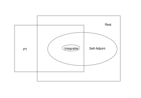
Fig. 1. : Relations among point interactions according to integrability.

We have presented a complete picture of self-adjoint, PT-symmetric and real spectrum point interactions, and their corresponding integrability. What we concerned here are just the case of particles with only pure contact interactions, and the possible contact coupling of the spins of two particles are not taken into account [15]. A further study along this direction would possibly give rise to more interesting integrable quantum many-body systems with various symmetries and spectrum properties.

References

-
[1]
C. M. Bender and S. Boettcher, Phys. Rev. Lett. 80,
5243 (1998).
C. M. Bender and S. Boettcher and P. N. Meisinger, J. Math. Phys. 40, 2201 (1999).
C. M. Bender, Dorje C. Brody, Hugh F. Jones Phys. Rev. Lett. 89, 270401 (2002). -
[2]
F. M. Fernández, R. Guardiola, J. Ros, and M. Znojil,
J. Phys. A: Math. Gen 31, 10105(1998).
A. Mostafazadeh, J. Math. Phys. 43, 205 (2002); 43, 2814 (2002); 43, 3944 (2002).
F. Cannata, G. Junker, and J. Trost, Phys. Lett. A 246, 219 (1998).
E. Delabaere and F. Pham, Phys. Lett A 250, 25 and 29 (1998).
C. M. Bender, G. V. Dunne, and P. N. Meisenger, Phys. Lett. A 252, 272 (1999).
C. M. Bender and G. V. Dunne, J. Math. Phys. 40, 4616 (1999).
M. Znojil, J. Phys. A: Math. Gen 32, 7419 (1999).
E. Delabaere and D. T. Trinh, J. Phys. A: Math. Gen 33, 8771 (2000).
A. Khare and B. P. Mandal, Phys. Lett. A 272, 53 (2000).
B. Bagchi, F. Cannata, and C. Quesne, Phys. Lett. A 269, 79(2000).
M. Znojil and M. Tater, J. Phys. A: Math. Gen 34, 1793 (2001).
B. Basu-Mallick and B. P. Mandal, Phys. Lett. A 284, 231 (2001).
M. Znojil, Phys. Lett. A 285, 7 (2001).
B. Bagchi, S. Mallik, and C. Quesne, Int. J. Mod. Phys. A 16, 2859 (2001).
C. M. Bender, G. V. Dunne, P. N. Meisenger, and M. Şimşek, Phys. Lett. A 281, 311(2001).
Z. Yan and C. R. Handy, J. Phys. A: Math. Gen 34, 9907 (2001).
Z. Ahmed, Phys. Lett. A 282, 343 (2001); 286, 231 (2001); 294 287 (2002).
C. M. Bender and Q. Wang, J. Phys. A 34, 3325 (2001). - [3] S. Albeverio, F. Gesztesy, R. Høegh-Krohn and H. Holden, Solvable Models in Quantum Mechanics, New York: Springer, 1988.
- [4] M. Gaudin, La fonction d’onde de Bethe, Masson, 1983.
- [5] S. Albeverio and R. Kurasov, Singular perturbations of differential operators and solvable Schrödinger type operators, London Mathematical Society Lecture Note Series, 271, Cambridge University Press, Cambridge, 2000.
- [6] P. Kurasov, J. Math. Analy. Appl. 201, 297-323 (1996).
-
[7]
J.B. McGuire,
J. Math. Phys. 5, 622-636 (1964); 6, 432-439 (1965);
7, 123-132 (1966).
J.B. McGuire and C.A. Hurst, J. Math. Phys. 13, 1595-1607 (1972); 29, 155-168 (1988). -
[8]
C.N. Yang, Phys. Rev. Lett. 19, 1312-1315 (1967).
C.N. Yang, Phys. Rev. 168, 1920-1923 (1968). - [9] C.H. Gu and C.N. Yang, Commun. Math. Phys. 122, 105-116 (1989).
- [10] P. Chernoff and R. Hughes, J. Func. Anal. 111, 97-117 (1993).
- [11] S. Albeverio, S.M. Fei and P. Kurasov, Lett. Math. Phys 59, 227-242 (2002).
- [12] S. Albeverio, Z. Brzeźniak and L Da̧browski, J. Phys. A27, 4933-4943 (1994).
- [13] S. Albeverio, L. Da̧browski and S.M. Fei, Int. J. Mod. Phys. B 14, 721-727 (2000).
-
[14]
Z.Q. Ma, Yang-Baxter Equation and Quantum Enveloping Algebras,
World Scientific, 1993.
V. Chari and A. Pressley, A Guide to Quantum Groups, Cambridge University Press, 1994.
C. Kassel, Quantum Groups, Springer-Verlag, New-York, 1995.
S. Majid, Foundations of Quantum Group Theory, Cambridge University Press, 1995.
K. Schmüdgen, Quantum Groups and Their Representations, Springer, 1997. - [15] S. Albeverio, S.M. Fei and P. Kurasov, Rep. Math. Phys. 47, 157-165 (2001).