Entanglement purification through Zeno-like measurements

Abstract

We present a novel method to purify quantum states, i.e. purification through Zeno-like measurements, and show an application to entanglement purification.

1 Introduction

One of the main obstacles to the experimental realisation of the ideas of quantum computation and quantum information is ‘decoherence’ [1, 2]. There are many attempts to overcome this problem, and several approaches are proposed for it. Among them are the ‘purification/distillation’ technologies [2, 3], i.e. methods to extract pure states, especially entanglements, from general mixed states recovering/preparing quantum coherence. Contributing to this subject, we have recently proposed a novel method to purify quantum states, i.e. purification through Zeno-like measurements [4]. Here we show that it is possible to apply it for extracting entanglement, which is the key resource to the fundamentals of quantum computation and information.

2 Purification through Zeno-like measurements

Let us recapitulate the framework of our purification [4]. We consider two quantum systems X and A interacting with each other. The total system is initially in a general mixed state $\varrho_{\mathrm{tot}}$, from which we try to extract a pure state in A. We first make a measurement on X to confirm that it is in a given state $|{\phi}\rangle_{\mathrm{X}}$. If it is found in the state $|{\phi}\rangle_{\mathrm{X}}$, the state of the total system is projected by the projection operator

$$\mathcal{O}=|{\phi}\rangle_{\mathrm{X}}\langle{\phi}|\otimes\openone_{\mathrm{A}}.$$ (1)

We then let the total system start to evolve under the Hamiltonian $H_{\mathrm{tot}}$ and repeat the same measurement on X at time intervals $\tau$. After $N$ repetitions of successful confirmations, the state of the total system, $\varrho_{\mathrm{tot}}^{(\tau)}(N)$, is given by

$$\varrho_{\mathrm{tot}}^{(\tau)}(N) = (\mathcal{O}e^{-iH_{\mathrm{tot}}\tau}\mathcal{O})^{N}\varrho_{\mathrm{tot}}(\mathcal{O}e^{iH_{\mathrm{tot}}\tau}\mathcal{O})^{N}/P^{(\tau)}(N)=|{\phi}\rangle_{\mathrm{X}}\langle{\phi}|\otimes\varrho_{\mathrm{A}}^{(\tau)}(N),$$ (2)

$$\varrho_{\mathrm{A}}^{(\tau)}(N) = \bm{(}V_{\phi}(\tau)\bm{)}^{N}\varrho_{\mathrm{A}}\bm{(}V_{\phi}^{\dagger}(\tau)\bm{)}^{N}/P^{(\tau)}(N),$$ (3)

where $\varrho_{\mathrm{A}}={}_{\mathrm{X}}\langle{\phi}|\varrho_{\mathrm{tot}}|{\phi}\rangle_{\mathrm{X}}$ is the state of A after the zeroth confirmation,

$$V_{\phi}(\tau)\equiv{}_{\mathrm{X}}\langle{\phi}|e^{-iH_{\mathrm{tot}}\tau}|{\phi}\rangle_{\mathrm{X}}$$ (4)

is a projected time-evolution operator, and $P^{(\tau)}(N)$ is the normalisation factor,

$$P^{(\tau)}(N)=\Tr[(\mathcal{O}e^{-iH_{\mathrm{tot}}\tau}\mathcal{O})^{N}\varrho_{\mathrm{tot}}(\mathcal{O}e^{iH_{\mathrm{tot}}\tau}\mathcal{O})^{N}]=\Tr_{\mathrm{A}}[\bm{(}V_{\phi}(\tau)\bm{)}^{N}\varrho_{\mathrm{A}}\bm{(}V_{\phi}^{\dagger}(\tau)\bm{)}^{N}].$$ (5)

Note that we retain only the events where X is found in the state $|{\phi}\rangle_{\mathrm{X}}$ at every measurement; other events, resulting in failure to purify A, are discarded. The normalisation factor $P^{(\tau)}(N)$ in (5) is nothing but the probability for the successful events and is the probability of obtaining the state given in (2) and (3).

Let us assume for simplicity that the eigenvalues $\lambda_{n}$ of $V_{\phi}(\tau)$, which are complex-valued in general, are discrete and $V_{\phi}(\tau)$ is decomposed (diagonalised) as

$$V_{\phi}(\tau)=\sum_{n}\lambda_{n}|{u_{n}}\rangle_{\mathrm{A}}\langle{v_{n}}|,$$ (6)

where $|{u_{n}}\rangle_{\mathrm{A}}$ and ${}_{\mathrm{A}}\langle{v_{n}}|$ are the right and left eigenvectors of $V_{\phi}(\tau)$, respectively, belonging to the eigenvalue $\lambda_{n}$ and satisfy ${}_{\mathrm{A}}\langle{v_{n}}|{u_{m}}\rangle_{\mathrm{A}}=\delta_{mn}$. (The right eigenvectors are normalised as ${}_{\mathrm{A}}\langle{u_{n}}|{u_{n}}\rangle_{\mathrm{A}}=1$ in the following.) It is now easy to observe the asymptotic behaviour of the state of A in (3). Since the eigenvalues $\lambda_{n}$ are bounded as $0\leq|\lambda_{n}|\leq 1$, each term in the expansion of $\bm{(}V_{\phi}(\tau)\bm{)}^{N}$ decays away and a single term dominates asymptotically as the number of measurements, $N$, increases,

$$\bm{(}V_{\phi}(\tau)\bm{)}^{N}=\sum_{n}\lambda_{n}^{N}|{u_{n}}\rangle_{\mathrm{A}}\langle{v_{n}}|\to\lambda_{0}^{N}|{u_{0}}\rangle_{\mathrm{A}}\langle{v_{0}}|\quad\mbox{as $N$ increases},$$ (7)

provided the largest (in magnitude) eigenvalue $\lambda_{0}$ is unique, discrete and nondegenerate. Then, the state of A in (3) accordingly approaches the pure state $|{u_{0}}\rangle_{\mathrm{A}}$,

$$\varrho_{\mathrm{A}}^{(\tau)}(N)\to|{u_{0}}\rangle_{\mathrm{A}}\langle{u_{0}}|\quad\mbox{as $N$ increases}.$$ (8)

This is the purification we have found recently [4]: extraction of a pure state $|{u_{0}}\rangle_{\mathrm{A}}$ from an arbitrary mixed state $\varrho_{\mathrm{A}}$ through repeated measurements on X. Since we repeat measurements (on X) as in the case of the quantum Zeno effect [5], we call such measurements ‘Zeno-like measurements’.

The above observation shows that the assumption of the ‘spectral decomposition’ (6) is not essential but the existence of the unique, discrete and nondegenerate largest eigenvalue $\lambda_{0}$ is crucial for the purification. Furthermore, note the asymptotic behaviour of the ‘success probability’ $P^{(\tau)}(N)$: it decays asymptotically as

$$P^{(\tau)}(N)\to|\lambda_{0}|^{2N}{}_{\mathrm{A}}\langle{v_{0}}|\varrho_{\mathrm{A}}|{v_{0}}\rangle_{\mathrm{A}}\quad\mbox{as $N$ increases},$$ (9)

which is dominated by the eigenvalue $\lambda_{0}$. Efficient purification is possible if it satisfies the condition $|\lambda_{0}|=1$, which suppresses the decay in (9). At the same time, if the other eigenvalues are much smaller than $\lambda_{0}$ in magnitude, purification is achieved faster. Hence,

$$|\lambda_{0}|=1,\qquad|\lambda_{n}/\lambda_{0}|\ll 1\quad\mathrm{for}\quad n\neq 0$$ (10)

are the conditions for the efficient purification, which we try to achieve by adjusting parameters such as $\tau$, $|{\phi}\rangle_{\mathrm{X}}$ and those in the Hamiltonian $H_{\mathrm{tot}}$.

3 Application to entanglement purification

Now we show an interesting application of the above scheme: application to entanglement purification. Let us consider, for example, a three-qubit system with the Hamiltonian

$$H_{\mathrm{tot}}=\Omega\frac{1+\sigma_{3}^{\mathrm{X}}}{2}+\Omega\frac{1+\sigma_{3}^{\mathrm{A}}}{2}+\Omega\frac{1+\sigma_{3}^{\mathrm{B}}}{2}+g(\sigma_{+}^{\mathrm{X}}\sigma_{-}^{\mathrm{A}}+\sigma_{-}^{\mathrm{X}}\sigma_{+}^{\mathrm{A}})+g(\sigma_{+}^{\mathrm{X}}\sigma_{-}^{\mathrm{B}}+\sigma_{-}^{\mathrm{X}}\sigma_{+}^{\mathrm{B}}),$$ (11)

where $\sigma_{i}\,(i=1,2,3)$ are the Pauli operators and $\sigma_{\pm}=(\sigma_{1}\pm i\sigma_{2})/2$ are the ladder operators. Qubit X is coupled to qubits A and B. We confirm X to be in the state $|{\phi}\rangle_{\mathrm{X}}$ repeatedly at time intervals $\tau$ and end up with an extraction of an entanglement between A and B, which are initially in a general mixed state $\varrho_{\mathrm{tot}}$.

The projected time-evolution operator $V_{\phi}(\tau)$ is given, in this case, by

$$V_{\phi}(\tau) = |{\Psi^{-}}\rangle_{\mathrm{AB}}\langle{\Psi^{-}}|\,\bigl{(}|\beta|^{2}+|\alpha|^{2}e^{-i\Omega\tau}\bigr{)}\,e^{-i\Omega\tau}$$ (12)

$${}+|{\downarrow\downarrow}\rangle_{\mathrm{AB}}\langle{\downarrow\downarrow}|\,\bigl{(}|\beta|^{2}+|\alpha|^{2}e^{-i\Omega\tau}\cos\sqrt{2}g\tau\bigr{)}$$

$${}+|{\Psi^{+}}\rangle_{\mathrm{AB}}\langle{\Psi^{+}}|\,\bigl{(}|\beta|^{2}+|\alpha|^{2}e^{-i\Omega\tau}\bigr{)}\,e^{-i\Omega\tau}\cos\sqrt{2}g\tau$$

$${}+|{\uparrow\uparrow}\rangle_{\mathrm{AB}}\langle{\uparrow\uparrow}|\,\bigl{(}|\beta|^{2}\cos\sqrt{2}g\tau+|\alpha|^{2}e^{-i\Omega\tau}\bigr{)}\,e^{-i2\Omega\tau}$$

$${}-i\,\bigl{(}\alpha^{*}\beta|{\downarrow\downarrow}\rangle_{\mathrm{AB}}\langle{\Psi^{+}}|+\alpha\beta^{*}|{\Psi^{+}}\rangle_{\mathrm{AB}}\langle{\downarrow\downarrow}|\bigr{)}\,e^{-i\Omega\tau}\sin\sqrt{2}g\tau$$

$${}-i\,\bigl{(}\alpha\beta^{*}|{\uparrow\uparrow}\rangle_{\mathrm{AB}}\langle{\Psi^{+}}|+\alpha^{*}\beta|{\Psi^{+}}\rangle_{\mathrm{AB}}\langle{\uparrow\uparrow}|\bigr{)}\,e^{-i2\Omega\tau}\sin\sqrt{2}g\tau,$$

where $|{\Psi^{\pm}}\rangle_{\mathrm{AB}}=(|{\uparrow\downarrow}\rangle_{\mathrm{AB}}\pm|{\downarrow\uparrow}\rangle_{\mathrm{AB}})/\sqrt{2}$ and $|{\phi}\rangle_{\mathrm{X}}=\alpha|{\uparrow}\rangle_{\mathrm{X}}+\beta|{\downarrow}\rangle_{\mathrm{X}}$, with $|{{\uparrow}({\downarrow})}\rangle$ the eigenstates of $\sigma_{3}$ belonging to the eigenvalues $+1\,(-1)$. Since the Hamiltonian (11) is symmetric under the exchange between A and B, $V_{\phi}(\tau)$ splits into the singlet and triplet sectors, and the singlet state $|{\Psi^{-}}\rangle_{\mathrm{AB}}$ is one of the four eigenstates of $V_{\phi}(\tau)$. It is hence possible to extract a Bell state $|{\Psi^{-}}\rangle_{\mathrm{AB}}$ provided (i) the corresponding eigenvalue

$$\lambda_{\Psi^{-}}=e^{-i\Omega\tau}\,\bigl{(}|\beta|^{2}+|\alpha|^{2}e^{-i\Omega\tau}\bigr{)}$$ (13)

is larger (in magnitude) than any other eigenvalue, and the extraction is efficient if the conditions (10), i.e. (ii) $|\lambda_{\Psi^{-}}|=1$ and (iii) $|\lambda_{n}/\lambda_{\Psi^{-}}|\ll 1\,(n\neq\Psi^{-})$, are fulfilled.

Condition (ii) is achieved by tuning $\tau$ such as

$$|\Omega|\tau=2n\pi\quad(n=0,1,2,\ldots),$$ (14)

and condition (i) is possible unless $|{\phi}\rangle_{\mathrm{X}}=|{\uparrow}\rangle_{\mathrm{X}}$ or $|{\downarrow}\rangle_{\mathrm{X}}$. Let us hence consider, under the condition (14), the case where

$$\alpha=\beta=1/\sqrt{2},\quad\mbox{i.e.}\quad|{\phi}\rangle_{\mathrm{X}}=|{\rightarrow}\rangle_{\mathrm{X}}\equiv\bigl{(}|{\uparrow}\rangle_{\mathrm{X}}+|{\downarrow}\rangle_{\mathrm{X}}\bigr{)}/\sqrt{2}.$$ (15)

In this case, three other eigenvalues than $\lambda_{\Psi^{-}}$ are given by

$$\lambda_{\Phi^{-}}=\cos^{2}\!\frac{g\tau}{\sqrt{2}},\quad\lambda_{\pm}=1-\frac{1}{2}\sin\frac{g\tau}{\sqrt{2}}\left(3\sin\frac{g\tau}{\sqrt{2}}\pm\sqrt{1-9\cos^{2}\!\frac{g\tau}{\sqrt{2}}}\right),$$ (16)

whose magnitudes are less than $1$, fulfilling condition (i), when

$$|g|\tau/\sqrt{2}\neq m\pi/2\quad(m=0,1,2,\ldots).$$ (17)

Therefore, the set of such parameters as (14), (15) and (17) enables us to extract the Bell state $|{\Psi^{-}}\rangle_{\mathrm{AB}}$ from a general mixed state $\varrho_{\mathrm{tot}}$.

The extraction of the Bell state $|{\Psi^{-}}\rangle_{\mathrm{AB}}$ is demonstrated in figure 1, where the fidelity to the target state $|{\Psi^{-}}\rangle_{\mathrm{AB}}$, defined by $F^{(\tau)}(N)\equiv{}_{\mathrm{AB}}\langle{\Psi^{-}}|\varrho_{\mathrm{AB}}^{(\tau)}(N)|{\Psi^{-}}\rangle_{\mathrm{AB}}$, and the success probability $P^{(\tau)}(N)$ versus the number of measurements, $N$, are shown for the initial state $\varrho_{\mathrm{tot}}=|{\rightarrow}\rangle_{\mathrm{X}}\langle{\rightarrow}|\otimes|{\uparrow}\rangle_{\mathrm{A}}\langle{\uparrow}|\otimes|{\downarrow}\rangle_{\mathrm{B}}\langle{\downarrow}|$, a (pure but) product state [or for a mixed state $\varrho_{\mathrm{tot}}=|{\rightarrow}\rangle_{\mathrm{X}}\langle{\rightarrow}|\otimes(|{\uparrow\downarrow}\rangle_{\mathrm{AB}}\langle{\uparrow\downarrow}|+|{\downarrow\uparrow}\rangle_{\mathrm{AB}}\langle{\downarrow\uparrow}|)/2$].

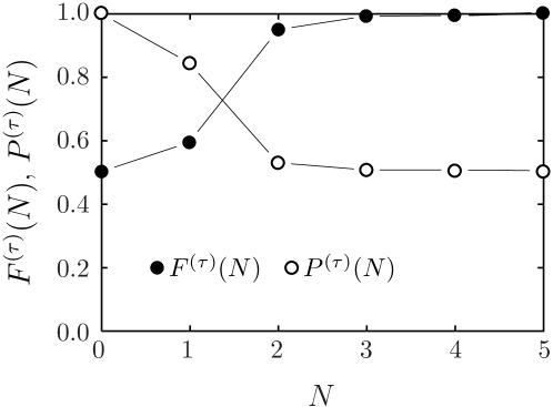
Figure 1: Extraction of a Bell state $|{\Psi^{-}}\rangle_{\mathrm{AB}}$ from a product state $\varrho_{\mathrm{tot}}=|{\rightarrow}\rangle_{\mathrm{X}}\langle{\rightarrow}|\otimes|{\uparrow}\rangle_{\mathrm{A}}\langle{\uparrow}|\otimes|{\downarrow}\rangle_{\mathrm{B}}\langle{\downarrow}|$ [or from a mixed state $\varrho_{\mathrm{tot}}=|{\rightarrow}\rangle_{\mathrm{X}}\langle{\rightarrow}|\otimes(|{\uparrow\downarrow}\rangle_{\mathrm{AB}}\langle{\uparrow\downarrow}|+|{\downarrow\uparrow}\rangle_{\mathrm{AB}}\langle{\downarrow\uparrow}|)/2$]. Parameters are $\tau=2\pi/\Omega$, $|{\phi}\rangle_{\mathrm{X}}=|{\rightarrow}\rangle_{\mathrm{X}}$ and $g=0.25\Omega$ ($\Omega>0$).

It is clear that the Bell state $|{\Psi^{-}}\rangle_{\mathrm{AB}}$ is extracted after only $4$ or $5$ measurements (in this case, $|\lambda_{\Phi^{-}}|\simeq 0.20$ and $|\lambda_{\pm}|\simeq 0.44$). Since condition (ii) is fulfilled, the decay of the success probability $P^{(\tau)}(N)$ is suppressed, yielding $P^{(\tau)}(N)\to{}_{\mathrm{AB}}\langle{\Psi^{-}}|\varrho_{\mathrm{AB}}|{\Psi^{-}}\rangle_{\mathrm{AB}}$ ($=1/2$ in figure 1), which means that the $|{\Psi^{-}}\rangle_{\mathrm{AB}}$ component contained in the initial state $\varrho_{\mathrm{AB}}$ (after the zeroth measurement on $\varrho_{\mathrm{tot}}$) is fully extracted. In this sense, the extraction is optimal.

4 Concluding remarks

The above example clearly and explicitly shows that our purification scheme works for entanglement purification. It is quite simple: one has simply to repeat one and the same measurement. At the same time, the purification can be made optimal: the optimal success probability is attainable as in the above example. Since the basic framework presented in section 2 is general, it possesses wide potential applicabilities in various settings for quantum computation and quantum information.

References

References

[1]Nielsen, M. A., and
Chuang, I. L.,
2000, Quantum Computation and Quantum Information
(Cambridge: Cambridge University Press),
and references therein.
[2]Bouwmeester, D.,
Ekert, A., and
Zeilinger, A.,
2000, The Physics of Quantum Information
(Heidelberg: Springer-Verlag),
and references therein.
[3]Bennett, C. H.,
Brassard, G.,
Popescu, S.,
Schumacher, B.,
Smolin, J. A., and
Wootters, W. K.,
1996, Phys. Rev. Lett., 76, 722;
Bennett, C. H.,
DiVincenzo, D. P.,
Smolin, J. A., and
Wootters, W. K.,
1996, Phys. Rev. A, 54, 3824.
[4]Nakazato, H.,
Takazawa, T., and
Yuasa, K.,
2003, Phys. Rev. Lett., 90, 060401.
[5]
For reviews, see:
Nakazato, H.,
Namiki, M., and
Pascazio, S.,
1996, Int. J. Mod. Phys. B, 10, 247;
Home, D., and
Whitaker, M. A. B.,
1997, Ann. Phys. (N.Y.), 258, 237;
Facchi, P., and
Pascazio, S.,
2001,
in Progress in Optics,
edited by E. Wolf (Amsterdam: Elsevier),
Vol. 42, p. 147.