Preparation and entanglement purification of qubits through Zeno-like measurements

Abstract

A novel method of purification, purification through Zeno-like measurements [H. Nakazato, T. Takazawa, and K. Yuasa, Phys. Rev. Lett. 90, 060401 (2003)], is discussed extensively and applied to a few simple qubit systems. It is explicitly demonstrated how it works and how it is optimized. As possible applications, schemes for initialization of multiple qubits and entanglement purification are presented, and their efficiency is investigated in detail. Simplicity and flexibility of the idea allow us to apply it to various kinds of settings in quantum information and computation, and would provide us with useful and practical methods of state preparation.

I Introduction

It is usually not seriously discussed in normal textbooks on quantum mechanics about how to prepare an initial state. It is, however, becoming an important subject not only from a view point of foundation of quantum mechanics, but also from a practical point of view, since we are rushing towards experimental realizations of the ideas for quantum information and computation ref:QuantInfoCompChuang ; ref:QuantInfoCompZeilinger . Without establishing particular initial states assumed in several algorithms, we cannot start any processes of the attractive ideas. State preparation is one of the key elements to quantum information processing ref:QuantInfoCompChuang ; ref:QuantInfoCompZeilinger , and there are several theoretical proposals ref:StatePreparationTh ; ref:EntanglementPreparationTh ; ref:EntanglementSeparate and experimental attempts ref:Haroche1997 ; ref:NIST ; ref:Blatt ; ref:NEC ; ref:YamamotoNumberState2003 .

In the ideas for quantum information and computation, quantum states with high coherence, especially entangled states, play significant and essential roles. But such “clean” states required for quantum information technologies are not easily found in nature, since many of them are fragile against environmental perturbations and suffer from decoherence. Therefore, there would often be a demand for preparing a desired pure state out of an arbitrary mixed state. Several schemes have been proposed for it, which are called “purification,” “distillation,” “concentration,” “extraction,” etc. ref:QuantInfoCompZeilinger ; ref:PurificationBennett ; ref:PurificationExperiments .

One of the simplest and easiest ways of state preparation is to resort to a projective measurement: a quantum system shall be in a pure state $|{\phi}\rangle$ after it is measured and confirmed to be in the state $|{\phi}\rangle$. Such a strategy is not possible, however, in cases where the desired state $|{\phi}\rangle$ cannot be directly measured or where the relevant system is not available after the confirmation. This is often the case for entangled states, which are the key resources to quantum information and computation. This is why more elaborate purification protocols are required and several schemes of entanglement purification/ preparation have been proposed ref:QuantInfoCompZeilinger ; ref:PurificationBennett ; ref:PurificationExperiments .

Recently, a novel mechanism to purify quantum states has been found and reported: purification through Zeno-like measurements ref:qpf . A pure state is extracted in a quantum system through a series of repeated measurements (Zeno-like measurements) on another quantum system in interaction with the former. Since the relevant system to be purified is not directly measured in this scheme, it would be suitable for such situations mentioned above. In this article, we discuss this scheme in detail and explore, on a heuristic basis, its potential as a useful and effective method of purification of qubits. The examples considered here are quite simple but still possess potential and practical applicability.

This article is organized as follows. First, the basic framework of the purification is described in a general setting, and the conditions for the purification and its optimization are summarized in Sec. II, where some details which are not discussed in the first report ref:qpf are included. It is then demonstrated in Sec. III how it works and how it can be made optimal in a simplest example, i.e., single-qubit purification, and a generalization to a multi-qubit case is considered in Sec. IV, which would afford us a useful method of initialization of multiple qubits. One of the interesting applications of the present scheme is entanglement purification, which is discussed in Sec. V and shown to be actually possible. Concluding remarks are given in Sec. VI with some comments on possible extensions and future subjects. Appendices A–E are supplied in order to demonstrate detailed calculations and proofs, that are not described in the text.

II Framework

Let us recapitulate the framework of the purification reported in ref:qpf . We consider two quantum systems X and A interacting with each other (Fig. 1).

Figure 1: We repeat measurements on X and purify A.

The total system X+A is initially in a mixed state $\varrho_{\text{tot}}$, from which we try to extract a pure state in A by controlling X. We first perform a measurement on X (the zeroth measurement) to confirm that it is in a state $|{\phi}\rangle_{\text{X}}$. If it is found in the state $|{\phi}\rangle_{\text{X}}$, the state of the total system is projected by the projection operator

$$\mathcal{O}=|{\phi}\rangle_{\text{X}}\langle{\phi}|\otimes\openone_{\text{A}}$$ (1)

to yield

$$\varrho_{\text{tot}}\to\tilde{\varrho}_{\text{tot}}=\frac{\mathcal{O}\varrho_{\text{tot}}\mathcal{O}}{\mathop{\text{Tr}}\nolimits(\mathcal{O}\varrho_{\text{tot}}\mathcal{O})}=|{\phi}\rangle_{\text{X}}\langle{\phi}|\otimes\varrho_{\text{A}},$$ (2)

where $\varrho_{\text{A}}\equiv{}_{\text{X}}\langle{\phi}|\varrho_{\text{tot}}|{\phi}\rangle_{\text{X}}/P_{0}$ is the state of A after this zeroth confirmation and $P_{0}\equiv\mathop{\text{Tr}}\nolimits(\mathcal{O}\varrho_{\text{tot}}\mathcal{O})$ is the probability for this to happen. We then let the total system start to evolve under a total Hamiltonian $H_{\text{tot}}$ and repeat the same measurement on X at regular time intervals $\tau$. After $N$ repetitions of successful confirmations, i.e., after X is confirmed to be in the state $|{\phi}\rangle_{\text{X}}$ successively $N$ times, the state of the total system, $\varrho_{\text{tot}}^{(\tau)}(N)$, is cast into the following form:

$$\varrho_{\text{tot}}^{(\tau)}(N) =(\mathcal{O}e^{-iH_{\text{tot}}\tau})^{N}\tilde{\varrho}_{\text{tot}}(e^{iH_{\text{tot}}\tau}\mathcal{O})^{N}/\tilde{P}^{(\tau)}(N)$$

$$=|{\phi}\rangle_{\text{X}}\langle{\phi}|\otimes\varrho_{\text{A}}^{(\tau)}(N),$$ (3a)

$$\varrho_{\text{A}}^{(\tau)}(N) =\bm{(}V_{\phi}(\tau)\bm{)}^{N}\varrho_{\text{A}}\bm{(}V_{\phi}^{\dagger}(\tau)\bm{)}^{N}/\tilde{P}^{(\tau)}(N),$$ (3b)

where $V_{\phi}(\tau)$, defined by

$$V_{\phi}(\tau)\equiv{}_{\text{X}}\langle{\phi}|e^{-iH_{\text{tot}}\tau}|{\phi}\rangle_{\text{X}},$$ (4)

is a projected time-evolution operator acting on the Hilbert space of A, and $\tilde{P}^{(\tau)}(N)$ is the normalization factor,

$$\tilde{P}^{(\tau)}(N) =\mathop{\text{Tr}}\nolimits[(\mathcal{O}e^{-iH_{\text{tot}}\tau})^{N}\tilde{\varrho}_{\text{tot}}(e^{iH_{\text{tot}}\tau}\mathcal{O})^{N}]$$

$$=\mathop{\text{Tr}}\nolimits_{\text{A}}[\bm{(}V_{\phi}(\tau)\bm{)}^{N}\varrho_{\text{A}}\bm{(}V_{\phi}^{\dagger}(\tau)\bm{)}^{N}].$$ (5)

Note that we retain only those events where X is found in the state $|{\phi}\rangle_{\text{X}}$ at every measurement (including the zeroth one); other events, resulting in failure to purify A, are discarded. The normalization factor $\tilde{P}^{(\tau)}(N)$ multiplied by $P_{0}$, i.e., $P^{(\tau)}(N)\equiv\tilde{P}^{(\tau)}(N)P_{0}$, is nothing but the probability for the successful events and is the probability of obtaining the state given in (3).

For definiteness, let us restrict ourselves on finite-dimensional systems throughout this article and consider the spectral decomposition of the operator $V_{\phi}(\tau)$. Since the operator $V_{\phi}(\tau)$ is not a Hermitian operator, we should set up both right and left eigenvalue equations

$$V_{\phi}(\tau)|{u_{n}}\rangle_{\text{A}} =\lambda_{n}|{u_{n}}\rangle_{\text{A}},$$ (6a)

$${}_{\text{A}}\langle{v_{n}}|V_{\phi}(\tau) =\lambda_{n}\,{}_{\text{A}}\langle{v_{n}}|.$$ (6b)

The eigenvalues $\lambda_{n}$ are complex in general and bounded as

$$0\leq|\lambda_{n}|\leq 1$$ (7)

(see Appendix A). Here we assume for simplicity that the spectrum of the operator $V_{\phi}(\tau)$ is not degenerate. In such a case, the eigenvectors are orthogonal to each other in the sense

$${}_{\text{A}}\langle{v_{m}}|{u_{n}}\rangle_{\text{A}}=\delta_{mn}$$ (8a)

and form a complete set in the Hilbert space of system A,

$$\sum_{n}|{u_{n}}\rangle_{\text{A}}\langle{v_{n}}|=\openone_{\text{A}},$$ (8b)

which readily leads to the spectral decomposition of the operator $V_{\phi}(\tau)$,

$$V_{\phi}(\tau)=\sum_{n}\lambda_{n}|{u_{n}}\rangle_{\text{A}}\langle{v_{n}}|.$$ (9)

(In the following, we also normalize the right eigenvectors as ${}_{\text{A}}\langle{u_{n}}|{u_{n}}\rangle_{\text{A}}=1$.)

Even in a general situation where the spectrum of the operator $V_{\phi}(\tau)$ is degenerate, the diagonalization (9) is possible when and only when all the right eigenvectors $|{u_{n}}\rangle_{\text{A}}$ are linearly independent of each other and form a complete basis ref:Kato . Otherwise, the spectral decomposition is not like (9), but in the “Jordan canonical form” ref:Kato . The diagonalizability of the operator $V_{\phi}(\tau)$ is, however, not an essential assumption as clarified in Appendix B.

It is now easy to observe the asymptotic behavior of the state of A, $\varrho_{\text{A}}^{(\tau)}(N)$ in (3b). Since the eigenvalues $\lambda_{n}$ are bounded like (7), each term in the expansion

$$\bm{(}V_{\phi}(\tau)\bm{)}^{N}=\sum_{n}\lambda_{n}^{N}|{u_{n}}\rangle_{\text{A}}\langle{v_{n}}|$$ (10)

decays out and a single term dominates asymptotically as the number of measurements, $N$, increases,

$$\bm{(}V_{\phi}(\tau)\bm{)}^{N}\to\lambda_{0}^{N}|{u_{0}}\rangle_{\text{A}}\langle{v_{0}}|\quad\mbox{as $N$ increases},$$ (11)

provided

$$\text{{the largest (in magnitude) eigenvalue $\lambda_{0}$ is}}\\[-3.0pt] \text{{unique, discrete and non\-degenerate}}.$$ (12)

[The word “unique” means that there is only one eigenvalue that has the maximum modulus and “nondegenerate” means that there is only one right eigenvector (and a corresponding left eigenvector) belonging to that maximal (in magnitude) eigenvalue.] Thus, the state of A in (3b) approaches a pure state $|{u_{0}}\rangle_{\text{A}}$,

$$\varrho_{\text{A}}^{(\tau)}(N)\to|{u_{0}}\rangle_{\text{A}}\langle{u_{0}}|\quad\mbox{as}\quad N\to\infty.$$ (13)

This is the purification scheme proposed recently ref:qpf : extraction of a pure state $|{u_{0}}\rangle_{\text{A}}$ through a series of repeated measurements on X. Since we repeat measurements (on X) as in the case of the quantum Zeno effect ref:QZE , we call such measurements “Zeno-like measurements” note:QZE . The final pure state $|{u_{0}}\rangle_{\text{A}}$ is the eigenstate of the projected time-evolution operator $V_{\phi}(\tau)$ belonging to the largest (in magnitude) eigenvalue $\lambda_{0}$ and depends on the parameters $\tau$, $|{\phi}\rangle_{\text{X}}$, and those in the Hamiltonian $H_{\text{tot}}$. It is, however, independent of the initial state $\varrho_{\text{tot}}$. The pure state $|{u_{0}}\rangle_{\text{A}}$ is extracted from an arbitrary mixed state $\varrho_{\text{tot}}$ through the Zeno-like measurements. By tuning such parameters mentioned above, we have a possibility of extracting a desired pure state $|{u_{0}}\rangle_{\text{A}}$.

The above observation shows that the assumption of the diagonalizability in (9) is not essential but condition (12), i.e., the existence of the unique, discrete and nondegenerate largest (in magnitude) eigenvalue $\lambda_{0}$, is crucial to the purification. For our purification mechanism to work, it is crucial that a single state is extracted and this is accomplished when these qualifications, i.e., the uniqueness of the largest eigenvalue and the nondegeneracy of the eigenvector, are both met. The diagonalizability of $V_{\phi}(\tau)$ is not relevant to these conditions and is not essential to the purification. This point is clarified in Appendix B.

Furthermore, note the asymptotic behavior of the success probability $P^{(\tau)}(N)$: it decays asymptotically as

$$P^{(\tau)}(N)\to{} |\lambda_{0}|^{2N}P_{0}\,{}_{\text{A}}\langle{v_{0}}|\varrho_{\text{A}}|{v_{0}}\rangle_{\text{A}}$$

$$={} |\lambda_{0}|^{2N}{}_{\text{XA}}\langle{\phi v_{0}}|\varrho_{\text{tot}}|{\phi v_{0}}\rangle_{\text{XA}}\quad\mbox{as $N$ increases},$$ (14)

where $|{\phi u_{0}}\rangle_{\text{XA}}$ stands for $|{\phi}\rangle_{\text{X}}\otimes|{u_{0}}\rangle_{\text{A}}$ and ${}_{\text{XA}}\langle{\phi u_{0}}|={}_{\text{X}}\langle{\phi}|\otimes{}_{\text{A}}\langle{u_{0}}|$. The decay is governed by the eigenvalue $\lambda_{0}$, and therefore, an efficient purification is possible if $\lambda_{0}$ satisfies the condition

$$|\lambda_{0}|=1,$$ (15)

which suppresses the decay in (14) to give the final (nonvanishing) success probability

$$P^{(\tau)}(N)\to{}_{\text{XA}}\langle{\phi v_{0}}|\varrho_{\text{tot}}|{\phi v_{0}}\rangle_{\text{XA}}.$$ (16)

It is worth stressing that the condition (15) allows us to repeat the measurement as many times as we wish without running the risk of losing the success probability $P^{(\tau)}(N)$. In other words, high fidelity to the target state and nonvanishing success probability do not contradict each other in this scheme, but rather they can be achieved simultaneously. At the same time, if the other eigenvalues are much smaller than $\lambda_{0}$ in magnitude,

$$|\lambda_{n}/\lambda_{0}|\ll 1\quad\text{for}\quad n\neq 0,$$ (17)

purification is achieved quickly. Equations (15) and (17) are the conditions for the optimal purification, which we try to accomplish by adjusting parameters $\tau$, $|{\phi}\rangle_{\text{X}}$, and those in the Hamiltonian $H_{\text{tot}}$.

In the following sections, we discuss the above purification scheme in more detail addressing a few specific examples, which are so simple but still possess potential and practical applications in quantum information and computation.

III Single-Qubit Purification

Let us first observe how the above mechanism works in the simplest example: we consider two qubits (two two-level systems) X and A interacting with each other, whose total Hamiltonian is given by

$$H_{\text{tot}}=\Omega_{\text{X}}\frac{1+\sigma_{3}^{\text{X}}}{2}+\Omega_{\text{A}}\frac{1+\sigma_{3}^{\text{A}}}{2}+g(\sigma_{+}^{\text{X}}\sigma_{-}^{\text{A}}+\sigma_{-}^{\text{X}}\sigma_{+}^{\text{A}}),$$ (18)

where $\sigma_{i}\,(i=1,2,3)$ are the Pauli operators, $\sigma_{\pm}=(\sigma_{1}\pm i\sigma_{2})/2$ are the ladder operators, and the frequencies $\Omega_{\text{X(A)}}$ and the coupling constant $g\,(\neq 0)$ are real parameters. We repeatedly confirm the state of X and purify qubit A, i.e., we discuss a purification of a single qubit.

The four eigenvalues of the total Hamiltonian $H_{\text{tot}}$ in (18) are given by

$$E^{(0)} =0,$$ (19a)

$$E^{(1)}_{\pm} =(\Omega_{\text{X}}+\Omega_{\text{A}})/2\pm\delta,$$ (19b)

$$E^{(2)} =\Omega_{\text{X}}+\Omega_{\text{A}},$$ (19c)

and the corresponding eigenstates are

$$|{E^{(0)}}\rangle_{\text{XA}}={} |{\downarrow\downarrow}\rangle_{\text{XA}},$$ (20a)

$$|{E^{(1)}_{\pm}}\rangle_{\text{XA}}={} \frac{1}{\sqrt{2}}\,\biggl{(}\epsilon(g)\sqrt{1\pm\frac{\Omega_{\text{X}}-\Omega_{\text{A}}}{2\delta}}|{\uparrow\downarrow}\rangle_{\text{XA}}$$

$$\phantom{\frac{1}{\sqrt{2}}\,\biggl{(}}{}\pm\sqrt{1\mp\frac{\Omega_{\text{X}}-\Omega_{\text{A}}}{2\delta}}|{\downarrow\uparrow}\rangle_{\text{XA}}\biggr{)},$$ (20b)

$$|{E^{(2)}}\rangle_{\text{XA}}={} |{\uparrow\uparrow}\rangle_{\text{XA}},$$ (20c)

where

$$\delta=\sqrt{(\Omega_{\text{X}}-\Omega_{\text{A}})^{2}/4+g^{2}},$$ (21)

$\epsilon(g)$ is the sign function, and $|{{\uparrow}({\downarrow})}\rangle$ is the eigenstate of the operator $\sigma_{3}$ belonging to the eigenvalue $+1\,(-1)$ with the phase convention $|{\uparrow}\rangle=\sigma_{+}|{\downarrow}\rangle$. Hence, when the state of X, $|{\phi}\rangle_{\text{X}}$, is confirmed repeatedly at time intervals $\tau$, the relevant operator to be investigated, the projected time-evolution operator $V_{\phi}(\tau)$, reads

$$V_{\phi}(\tau)\equiv{} {}_{\text{X}}\langle{\phi}|e^{-iH_{\text{tot}}\tau}|{\phi}\rangle_{\text{X}}$$

$$={} |{\uparrow}\rangle_{\text{A}}\langle{\uparrow}|e^{-i(\Omega_{\text{X}}+\Omega_{\text{A}})\tau}\left[\cos^{2}\!\frac{\theta}{2}+e^{i(\Omega_{\text{X}}+\Omega_{\text{A}})\tau/2}\left(\cos\delta\tau+i\frac{\Omega_{\text{X}}-\Omega_{\text{A}}}{2\delta}\sin\delta\tau\right)\sin^{2}\!\frac{\theta}{2}\right]$$

$${}+|{\downarrow}\rangle_{\text{A}}\langle{\downarrow}|\left[\sin^{2}\!\frac{\theta}{2}+e^{-i(\Omega_{\text{X}}+\Omega_{\text{A}})\tau/2}\left(\cos\delta\tau-i\frac{\Omega_{\text{X}}-\Omega_{\text{A}}}{2\delta}\sin\delta\tau\right)\cos^{2}\!\frac{\theta}{2}\right]$$

$${}-i\left(|{\uparrow}\rangle_{\text{A}}\langle{\downarrow}|e^{-i\varphi}+|{\downarrow}\rangle_{\text{A}}\langle{\uparrow}|e^{i\varphi}\right)\frac{g}{\delta}e^{-i(\Omega_{\text{X}}+\Omega_{\text{A}})\tau/2}\sin\delta\tau\sin\frac{\theta}{2}\cos\frac{\theta}{2},$$ (22)

where the state $|{\phi}\rangle_{\text{X}}$ is parameterized as

$$|{\phi}\rangle_{\text{X}}=e^{-i\varphi/2}\cos\frac{\theta}{2}|{\uparrow}\rangle_{\text{X}}+e^{i\varphi/2}\sin\frac{\theta}{2}|{\downarrow}\rangle_{\text{X}}$$ (23)

and the set of angles $(\theta,\varphi)$ characterizes the “direction of ‘spin’ X.”

If one of the two eigenvalues of the operator (22) is larger in magnitude than the other, the condition for purification (12) is fulfilled, and qubit A is purified into the eigenstate $|{u_{0}}\rangle_{\text{A}}$ belonging to the larger (in magnitude) eigenvalue $\lambda_{0}$. Furthermore, if condition (15), $|\lambda_{0}|=1$, is satisfied, we can purify with a nonvanishing success probability $P^{(\tau)}(N)\to{}_{\text{XA}}\langle{\phi v_{0}}|\varrho_{\text{tot}}|{\phi v_{0}}\rangle_{\text{XA}}$, and another condition (17), $|\lambda_{1}/\lambda_{0}|\ll 1$, enables us to accomplish quick purification. We try to achieve these conditions by tuning the parameters.

The first adjustment for the optimal purification is

$$\theta=0\ \text{or}\ \pi,\quad\text{i.e.},\quad|{\phi}\rangle_{\text{X}}=|{\uparrow}\rangle_{\text{X}}\ \text{or}\ |{\downarrow}\rangle_{\text{X}}$$ (24)

(see Appendix C). Actually, if we choose $|{\phi}\rangle_{\text{X}}=|{\uparrow}\rangle_{\text{X}}$, the eigenvalues of the projected time-evolution operator $V_{\phi}(\tau)$ are given by

$$\begin{cases}\lambda_{0}=e^{-i(\Omega_{\text{X}}+\Omega_{\text{A}})\tau},\\ \displaystyle\lambda_{1}=e^{-i(\Omega_{\text{X}}+\Omega_{\text{A}})\tau/2}\left(\cos\delta\tau-i\frac{\Omega_{\text{X}}-\Omega_{\text{A}}}{2\delta}\sin\delta\tau\right),\end{cases}$$ (25a)

and the eigenvectors belonging to them are

$$\begin{cases}|{u_{0}}\rangle_{\text{A}}=|{\uparrow}\rangle_{\text{A}},\\ |{u_{1}}\rangle_{\text{A}}=|{\downarrow}\rangle_{\text{A}},\end{cases}\quad\begin{cases}{}_{\text{A}}\langle{v_{0}}|={}_{\text{A}}\langle{\uparrow}|,\\ {}_{\text{A}}\langle{v_{1}}|={}_{\text{A}}\langle{\downarrow}|.\end{cases}$$ (25b)

It is clear that the magnitude of the eigenvalue $\lambda_{0}$ is unity and that of $\lambda_{1}$,

$$|\lambda_{1}|=\sqrt{1-\left(\frac{g}{\delta}\right)^{2}\sin^{2}\!\delta\tau},$$ (26)

is less than unity provided

$$\delta\tau\neq n\pi\quad(n=1,2,\ldots).$$ (27)

Both conditions (12) and (15) are thus satisfied, and according to the theory presented in Sec. II, we have an optimal purification

$$\begin{cases}\vskip 6.0pt plus 2.0pt minus 2.0pt\varrho_{\text{A}}^{(\tau)}(N)\to|{\uparrow}\rangle_{\text{A}}\langle{\uparrow}|,\\ P^{(\tau)}(N)\to{}_{\text{XA}}\langle{\uparrow\uparrow}|\varrho_{\text{tot}}|{\uparrow\uparrow}\rangle_{\text{XA}},\end{cases}\quad(N\to\infty).$$ (28)

After the repeated confirmations of the state $|{\uparrow}\rangle_{\text{X}}$, qubit A is purified into $|{\uparrow}\rangle_{\text{A}}$ with a nonvanishing probability ${}_{\text{XA}}\langle{\uparrow\uparrow}|\varrho_{\text{tot}}|{\uparrow\uparrow}\rangle_{\text{XA}}$. Similarly, another choice in (24), i.e., a series of repeated confirmations of the state $|{\downarrow}\rangle_{\text{X}}$, drives A into $|{\downarrow}\rangle_{\text{A}}$ with a nonvanishing probability ${}_{\text{XA}}\langle{\downarrow\downarrow}|\varrho_{\text{tot}}|{\downarrow\downarrow}\rangle_{\text{XA}}$:

$$\begin{cases}\vskip 6.0pt plus 2.0pt minus 2.0pt\varrho_{\text{A}}^{(\tau)}(N)\to|{\downarrow}\rangle_{\text{A}}\langle{\downarrow}|,\\ P^{(\tau)}(N)\to{}_{\text{XA}}\langle{\downarrow\downarrow}|\varrho_{\text{tot}}|{\downarrow\downarrow}\rangle_{\text{XA}},\end{cases}\quad(N\to\infty).$$ (29)

The final success probability ${}_{\text{XA}}\langle{\uparrow\uparrow}|\varrho_{\text{tot}}|{\uparrow\uparrow}\rangle_{\text{XA}}$ for the former choice $|{\phi}\rangle_{\text{X}}=|{\uparrow}\rangle_{\text{X}}$ or ${}_{\text{XA}}\langle{\downarrow\downarrow}|\varrho_{\text{tot}}|{\downarrow\downarrow}\rangle_{\text{XA}}$ for the latter $|{\phi}\rangle_{\text{X}}=|{\downarrow}\rangle_{\text{X}}$ means that the target state $|{\uparrow\uparrow}\rangle_{\text{XA}}$ or $|{\downarrow\downarrow}\rangle_{\text{XA}}$ contained in the initial state $\varrho_{\text{tot}}$ is fully extracted. In this sense, the purification is optimal.

The second adjustment is for the fastest purification, which is realized by the condition

$$\delta\tau=(n+1/2)\pi\quad(n=0,1,\ldots),$$ (30)

at which $|\lambda_{1}|$ in (26) is the smallest: $|\lambda_{1}|=|\Omega_{\text{X}}-\Omega_{\text{A}}|/2\delta$. We can achieve it by tuning the time interval $\tau$, for instance.

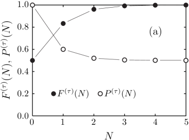
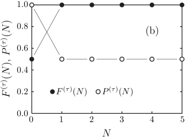
Figure 2: Fidelity $F^{(\tau)}(N)$ and success probability $P^{(\tau)}(N)$ for single-qubit purification. The pure state $|{{\uparrow}({\downarrow})}\rangle_{\text{A}}$ is extracted from the initial mixed state $\varrho_{\text{tot}}=|{{\uparrow}({\downarrow})}\rangle_{\text{X}}\langle{{\uparrow}({\downarrow})}|\otimes(|{\uparrow}\rangle_{\text{A}}\langle{\uparrow}|+|{\downarrow}\rangle_{\text{A}}\langle{\downarrow}|)/2$ after repeated confirmations of the state $|{{\uparrow}({\downarrow})}\rangle_{\text{X}}$. Parameters are $\Omega_{\text{X}}=5$, $\Omega_{\text{A}}=6$, $\tau=\pi/2\delta\simeq 1.40$ for (a) and $\Omega_{\text{X}}=\Omega_{\text{A}}$, $\tau=\pi/2\delta\simeq 1.57$ for (b), in the unit such that $g=1$. The time interval $\tau$ is tuned so as to satisfy the condition for the fastest purification (30) in each case.

To be more explicit, let us demonstrate the extraction of the pure state $|{\uparrow}\rangle_{\text{A}}$ from the initial mixed state

$$\varrho_{\text{tot}}=|{\uparrow}\rangle_{\text{X}}\langle{\uparrow}|\otimes\frac{1}{2}\left(|{\uparrow}\rangle_{\text{A}}\langle{\uparrow}|+|{\downarrow}\rangle_{\text{A}}\langle{\downarrow}|\right).$$ (31)

After X is confirmed to be in the state $|{\uparrow}\rangle_{\text{X}}$ successfully $N$ times at time intervals $\tau$, the state of qubit A and the probability for the successful confirmations read

$$\begin{cases}\vskip 6.0pt plus 2.0pt minus 2.0pt\displaystyle\varrho_{\text{A}}^{(\tau)}(N)=\frac{|{\uparrow}\rangle_{\text{A}}\langle{\uparrow}|+[1-(g/\delta)^{2}\sin^{2}\!\delta\tau]^{N}|{\downarrow}\rangle_{\text{A}}\langle{\downarrow}|}{1+[1-(g/\delta)^{2}\sin^{2}\!\delta\tau]^{N}},\\ \displaystyle P^{(\tau)}(N)=\frac{1}{2}\{1+[1-(g/\delta)^{2}\sin^{2}\!\delta\tau]^{N}\},\end{cases}$$ (32)

respectively, which clearly confirm the limits (28) unless $\delta\tau=n\pi$ ($n=1,2,\ldots$), and the convergences are the fastest when the condition (30) is satisfied. (Note that ${}_{\text{XA}}\langle{\uparrow\uparrow}|\varrho_{\text{tot}}|{\uparrow\uparrow}\rangle_{\text{XA}}=1/2$ for the initial state considered here.)

In Fig. 2(a), the success probability $P^{(\tau)}(N)$ and the so-called fidelity to the target state $|{u_{0}}\rangle_{\text{A}}=|{\uparrow}\rangle_{\text{A}}$, defined by

$$F^{(\tau)}(N) \equiv{}_{\text{A}}\langle{u_{0}}|\varrho_{\text{A}}^{(\tau)}(N)|{u_{0}}\rangle_{\text{A}}$$

$$={}_{\text{A}}\langle{\uparrow}|\varrho_{\text{A}}^{(\tau)}(N)|{\uparrow}\rangle_{\text{A}},$$ (33)

are shown as functions of the number of measurements, $N$, for the initial state (31), with the parameters $\Omega_{\text{X}}=5$, $\Omega_{\text{A}}=6$, $g=1$, $\tau=\pi/2\delta\simeq 1.40$. Since the condition (15), $|\lambda_{0}|=1$, is fulfilled, the decay of the success probability $P^{(\tau)}(N)$ is suppressed to yield the finite value ${}_{\text{XA}}\langle{\uparrow\uparrow}|\varrho_{\text{tot}}|{\uparrow\uparrow}\rangle_{\text{XA}}=1/2$, and since the time interval $\tau$ is tuned so as to satisfy the condition for the fastest purification (30) ($|\lambda_{1}|\simeq 0.45$), the pure state $|{\uparrow}\rangle_{\text{A}}$ is extracted after only $N=4$ or $5$ measurements. In an extreme case where $|\lambda_{1}|=0$ is possible, the extraction is achieved just after one measurement. Such a situation is depicted in Fig. 2(b) for the same initial state as in Fig. 2(a) with the parameter set $\Omega_{\text{X}}=\Omega_{\text{A}}$, $g=1$, $\tau=\pi/2\simeq 1.57$.

IV Initialization of Multiple Qubits

The single-qubit purification in the previous section is too simple but is easily extended for multi-qubit cases. In the above example, one may realize that the state $|{\uparrow\uparrow}\rangle_{\text{XA}}$ is an eigenstate of the total Hamiltonian (18) [see (20)] and this is why the optimization condition (15), $|\lambda_{0}|=1$, is achieved with $|{\phi}\rangle_{\text{X}}=|{\uparrow}\rangle_{\text{X}}$ and $|{u_{0}}\rangle_{\text{A}}=|{\uparrow}\rangle_{\text{A}}$ irrespectively of the choice of the time interval $\tau$. (The same argument applies to the case $|{\phi}\rangle_{\text{X}}=|{\downarrow}\rangle_{\text{X}}$ there.)

Figure 3: A multi-qubit system with nearest-neighbor interactions.

In the case of a multi-qubit system $\text{X}+\text{A}+\text{B}+\cdots$ in Fig. 3, with nearest-neighbor interactions,

$$H_{\text{tot}}={} \Omega_{\text{X}}\frac{1+\sigma_{3}^{\text{X}}}{2}+\Omega_{\text{A}}\frac{1+\sigma_{3}^{\text{A}}}{2}+\Omega_{\text{B}}\frac{1+\sigma_{3}^{\text{B}}}{2}+\cdots$$

$${}+g_{\text{XA}}(\sigma_{+}^{\text{X}}\sigma_{-}^{\text{A}}+\sigma_{-}^{\text{X}}\sigma_{+}^{\text{A}})+g_{\text{AB}}(\sigma_{+}^{\text{A}}\sigma_{-}^{\text{B}}+\sigma_{-}^{\text{A}}\sigma_{+}^{\text{B}})$$

$$\phantom{{}+{}}{}+\cdots$$ (34)

($g_{\text{XA}},g_{\text{AB}},\ldots\neq 0$), the state $|{{\uparrow\uparrow\uparrow}{\ldots}}\rangle_{\text{XAB\ldots}}$ is an eigenstate of this total Hamiltonian $H_{\text{tot}}$, and it is readily expected that the pure state $|{{\uparrow\uparrow}{\ldots}}\rangle_{\text{AB\ldots}}$ is extracted by repeated projections onto the state $|{\uparrow}\rangle_{\text{X}}$, with the optimal success probability. Similarly, repeated projections onto $|{\downarrow}\rangle_{\text{X}}$ set every qubit into $|{\downarrow}\rangle$ state, i.e., into $|{{\downarrow\downarrow}{\ldots}}\rangle_{\text{AB\ldots}}$, optimally. This would be useful for initialization of multiple qubits in a quantum computer.

In order to make this idea more concrete, let us discuss in detail with a three-qubit system $\text{X}+\text{A}+\text{B}$. The important point is whether the condition for the purification (12) is achievable, i.e., whether all the eigenvalues $\lambda_{n}$ except for the relevant one $\lambda_{0}$, associated with the eigenstate $|{\uparrow\uparrow}\rangle_{\text{AB}}$ (or $|{\downarrow\downarrow}\rangle_{\text{AB}}$), can actually be less than unity in magnitude.

For simplicity, we consider the case where $\Omega_{\text{X}}=\Omega_{\text{A}}=\Omega_{\text{B}}=\Omega$. The eight eigenvalues of the total Hamiltonian $H_{\text{tot}}$ are given by

$$E^{(0)} =0,$$ (35a)

$$E^{(1)}_{0} =\Omega, E^{(1)}_{\pm} =\Omega\pm\sqrt{2}\bar{g},$$ (35b)

$$E^{(2)}_{0} =2\Omega, E^{(2)}_{\pm} =2\Omega\pm\sqrt{2}\bar{g},$$ (35c)

$$E^{(3)} =3\Omega,$$ (35d)

and the corresponding eigenstates are

$$|{E^{(0)}}\rangle_{\text{XAB}}={} |{\downarrow\downarrow\downarrow}\rangle_{\text{XAB}},$$ (36a)

$$|{E^{(1)}_{0}}\rangle_{\text{XAB}}={} \cos\chi|{\downarrow\downarrow\uparrow}\rangle_{\text{XAB}}-\sin\chi|{\uparrow\downarrow\downarrow}\rangle_{\text{XAB}},$$ (36b)

$$|{E^{(1)}_{\pm}}\rangle_{\text{XAB}}={} \frac{1}{\sqrt{2}}(\sin\chi|{\downarrow\downarrow\uparrow}\rangle_{\text{XAB}}+\cos\chi|{\uparrow\downarrow\downarrow}\rangle_{\text{XAB}}$$

$$\phantom{\frac{1}{\sqrt{2}}(}{}\pm|{\downarrow\uparrow\downarrow}\rangle_{\text{XAB}}),$$ (36c)

$$|{E^{(2)}_{0}}\rangle_{\text{XAB}}={} \cos\chi|{\uparrow\uparrow\downarrow}\rangle_{\text{XAB}}-\sin\chi|{\downarrow\uparrow\uparrow}\rangle_{\text{XAB}},$$ (36d)

$$|{E^{(2)}_{\pm}}\rangle_{\text{XAB}}={} \frac{1}{\sqrt{2}}(\sin\chi|{\uparrow\uparrow\downarrow}\rangle_{\text{XAB}}+\cos\chi|{\downarrow\uparrow\uparrow}\rangle_{\text{XAB}}$$

$$\phantom{\frac{1}{\sqrt{2}}(}{}\pm|{\uparrow\downarrow\uparrow}\rangle_{\text{XAB}}),$$ (36e)

$$|{E^{(3)}}\rangle_{\text{XAB}}={} |{\uparrow\uparrow\uparrow}\rangle_{\text{XAB}},$$ (36f)

where

$$\sqrt{2}\bar{g}=\sqrt{g_{\text{XA}}^{2}+g_{\text{AB}}^{2}},$$ (37)

$$\cos\chi=\frac{g_{\text{XA}}}{\sqrt{g_{\text{XA}}^{2}+g_{\text{AB}}^{2}}},\quad\sin\chi=\frac{g_{\text{AB}}}{\sqrt{g_{\text{XA}}^{2}+g_{\text{AB}}^{2}}}.$$ (38)

Aiming at initializing qubits A and B into $|{\downarrow\downarrow}\rangle_{\text{AB}}$, we repeatedly project X onto the state $|{\downarrow}\rangle_{\text{X}}$ at time intervals $\tau$, and the relevant operator to be investigated reads

$$V_{\downarrow}(\tau)\equiv{} {}_{\text{X}}\langle{\downarrow}|e^{-iH_{\text{tot}}\tau}|{\downarrow}\rangle_{\text{X}}$$

$$={} |{\downarrow\downarrow}\rangle_{\text{AB}}\langle{\downarrow\downarrow}|$$

$${}+|{\uparrow\downarrow}\rangle_{\text{AB}}\langle{\uparrow\downarrow}|e^{-i\Omega\tau}\cos\sqrt{2}\bar{g}\tau$$

$${}+|{\downarrow\uparrow}\rangle_{\text{AB}}\langle{\downarrow\uparrow}|e^{-i\Omega\tau}(\cos^{2}\!\chi+\sin^{2}\!\chi\cos\sqrt{2}\bar{g}\tau)$$

$${}-i|{\uparrow\downarrow}\rangle_{\text{AB}}\langle{\downarrow\uparrow}|e^{-i\Omega\tau}\sin\chi\sin\sqrt{2}\bar{g}\tau$$

$${}-i|{\downarrow\uparrow}\rangle_{\text{AB}}\langle{\uparrow\downarrow}|e^{-i\Omega\tau}\sin\chi\sin\sqrt{2}\bar{g}\tau$$

$${}+|{\uparrow\uparrow}\rangle_{\text{AB}}\langle{\uparrow\uparrow}|e^{-2i\Omega\tau}(\sin^{2}\!\chi+\cos^{2}\!\chi\cos\sqrt{2}\bar{g}\tau).$$ (39)

The target state $|{\downarrow\downarrow}\rangle_{\text{AB}}$ is an eigenstate of this operator belonging to the eigenvalue $\lambda_{\downarrow\downarrow}=1$, which satisfies the optimization condition (15), and the other three eigenvalues are give by

$$\lambda_{\pm}={} e^{-i\Omega\tau}\biggl{(}\cos^{2}\!\frac{\bar{g}\tau}{\sqrt{2}}-\sin^{2}\!\chi\sin^{2}\!\frac{\bar{g}\tau}{\sqrt{2}}$$

$${}\mp\sin\frac{\bar{g}\tau}{\sqrt{2}}\sqrt{\cos^{4}\!\chi\sin^{2}\!\frac{\bar{g}\tau}{\sqrt{2}}-4\sin^{2}\!\chi\cos^{2}\!\frac{\bar{g}\tau}{\sqrt{2}}}\biggr{)},$$ (40a)

$$\lambda_{\uparrow\uparrow}={} e^{-2i\Omega\tau}\left(1-2\cos^{2}\!\chi\sin^{2}\!\frac{\bar{g}\tau}{\sqrt{2}}\right).$$ (40b)

If these three eigenvalues are all less than unity in magnitude, the condition for the purification (12) is satisfied, and the initialized state $|{\downarrow\downarrow}\rangle_{\text{AB}}$ is extracted from an arbitrary mixed state $\varrho_{\text{tot}}$, with a nonvanishing success probability $P^{(\tau)}(N)\to{}_{\text{XAB}}\langle{\downarrow\downarrow\downarrow}|\varrho_{\text{tot}}|{\downarrow\downarrow\downarrow}\rangle_{\text{XAB}}$. (Note that the left eigenvector belonging to the eigenvalue $\lambda_{\downarrow\downarrow}$ is ${}_{\text{AB}}\langle{\downarrow\downarrow}|$.) Such a situation is realized provided

$$\sqrt{2}\bar{g}\tau\neq n\pi\quad(n=1,2,\ldots),$$ (41)

which is clearly seen from Fig. 4 and a proof in Appendix D.

Figure 4: Magnitudes of the eigenvalues $\lambda_{+}$ (solid line), $\lambda_{-}$ (dashed line), and $\lambda_{\uparrow\uparrow}$ (dotted line) in (40), as functions of $\sqrt{2}\bar{g}\tau$. In this figure, we set $g_{\text{XA}}=g_{\text{AB}}$. Note that $|\lambda_{+}|=|\lambda_{-}|$ within each range $2n\pi-\zeta\leq\sqrt{2}\bar{g}\tau\leq 2n\pi+\zeta$ ($n=0,1,\ldots$), where $\zeta$ ($0<\zeta<\pi$) is defined by $\tan(\zeta/2)=2|\sin\chi|/\cos^{2}\!\chi$, and $\zeta\simeq 0.78\pi$ when $g_{\text{XA}}=g_{\text{AB}}$.

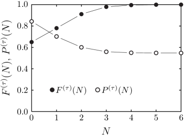
Figure 5: Fidelity $F^{(\tau)}(N)$ and success probability $P^{(\tau)}(N)$ for two-qubit initialization. Through the repeated confirmations of the state $|{\downarrow}\rangle_{\text{X}}$, qubits A and B are initialized into $|{\downarrow\downarrow}\rangle_{\text{AB}}$ from the thermal equilibrium state of the total system at temperature $T$, i.e., $\varrho_{\text{tot}}\propto e^{-\beta H_{\text{tot}}}$ with $\beta=(k_{\text{B}}T)^{-1}$. Parameters are $g_{\text{XA}}=g_{\text{AB}}=1$, $\Omega=2$, $\tau=\zeta/\sqrt{2}\simeq 1.73$, $k_{\text{B}}T=\beta^{-1}=1$. The time interval $\tau$ is tuned so as to make $\max(|\lambda_{+}|,|\lambda_{-}|,|\lambda_{\uparrow\uparrow}|)$ the smallest, which is for the fastest initialization (see Fig. 4).

The final success probability $P^{(\tau)}(N)\to{}_{\text{XAB}}\langle{\downarrow\downarrow\downarrow}|\varrho_{\text{tot}}|{\downarrow\downarrow\downarrow}\rangle_{\text{XAB}}$ is again optimal, in the sense that the target state $|{\downarrow\downarrow\downarrow}\rangle_{\text{XAB}}$ contained in the initial state $\varrho_{\text{tot}}$ is fully extracted.

The above argument reveals the possibility of initialization at least for two qubits. Initialization of two qubits into $|{\downarrow\downarrow}\rangle_{\text{AB}}$ from the thermal equilibrium state of the total system at temperature $T$, i.e., $\varrho_{\text{tot}}\propto e^{-\beta H_{\text{tot}}}$ with $\beta=(k_{\text{B}}T)^{-1}$, is demonstrated in Fig. 5. Note that it is effective when $\Omega>\sqrt{2}\bar{g}$, since in such a case, $|{\downarrow\downarrow\downarrow}\rangle_{\text{XAB}}$ is the ground state of the total system. The analytic formula for the final success probability is $P^{(\tau)}(\infty)=[1+(e^{-\beta\Omega}+e^{-2\beta\Omega})(1+2\cosh\sqrt{2}\beta\bar{g})+e^{-3\beta\Omega}]^{-1}$.

It is natural to expect that the same mechanism also works for systems with more qubits as in Fig. 3. It is hard to imagine that the magnitudes of eigenvalues of $V_{\downarrow}(\tau)$ other than the relevant one $\lambda_{\downarrow\downarrow\ldots}$ (whose magnitude is unity) is also unity irrespectively of the values of parameters. Further detailed investigations on its efficiency, robustness, and so on, will certainly clarify the possibility of a new useful procedure for initializing multiple qubits.

V Entanglement Purification

One of the most significant issues in the field of quantum information and computation is how to prepare entanglement, and therefore, it is interesting and important to examine whether the present scheme can realize entanglement purification/preparation. We show, in this section, that it is actually possible. In order to demonstrate it explicitly, let us discuss a simple Hamiltonian

$$H_{\text{tot}}={} \Omega\frac{1+\sigma_{3}^{\text{X}}}{2}+\Omega\frac{1+\sigma_{3}^{\text{A}}}{2}+\Omega\frac{1+\sigma_{3}^{\text{B}}}{2}$$

$${}+g(\sigma_{+}^{\text{X}}\sigma_{-}^{\text{A}}+\sigma_{-}^{\text{X}}\sigma_{+}^{\text{A}})+g(\sigma_{+}^{\text{X}}\sigma_{-}^{\text{B}}+\sigma_{-}^{\text{X}}\sigma_{+}^{\text{B}}).$$ (42)

The control qubit X is coupled to qubits A and B as in Fig. 6. We confirm X to be in the state $|{\phi}\rangle_{\text{X}}$ repeatedly at time intervals $\tau$ and end up with an extraction of an entanglement between A and B, which are initially in a mixed state $\varrho_{\text{tot}}$.

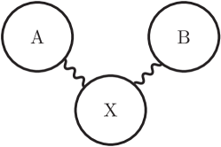
Figure 6: We repeat measurements on qubit X and extract one of the Bell states, $|{\Psi^{-}}\rangle_{\text{AB}}\equiv(|{\uparrow\downarrow}\rangle_{\text{AB}}-|{\downarrow\uparrow}\rangle_{\text{AB}})/\sqrt{2}$, in qubits A and B.

The spectrum of the total Hamiltonian $H_{\text{tot}}$ is already given in (35) with $\bar{g}$ replaced by $g$, and the eigenstates are

$$|{E^{(0)}}\rangle_{\text{XAB}}={} |{\downarrow\downarrow\downarrow}\rangle_{\text{XAB}},$$ (43a)

$$|{E^{(1)}_{0}}\rangle_{\text{XAB}}={} |{{\downarrow}\Psi^{-}}\rangle_{\text{XAB}},$$ (43b)

$$|{E^{(1)}_{\pm}}\rangle_{\text{XAB}}={} \frac{1}{\sqrt{2}}[|{{\downarrow}\Psi^{+}}\rangle_{\text{XAB}}\pm\epsilon(g)|{\uparrow\downarrow\downarrow}\rangle_{\text{XAB}}],$$ (43c)

$$|{E^{(2)}_{0}}\rangle_{\text{XAB}}={} |{{\uparrow}\Psi^{-}}\rangle_{\text{XAB}},$$ (43d)

$$|{E^{(2)}_{\pm}}\rangle_{\text{XAB}}={} \frac{1}{\sqrt{2}}[|{{\uparrow}\Psi^{+}}\rangle_{\text{XAB}}\pm\epsilon(g)|{\downarrow\uparrow\uparrow}\rangle_{\text{XAB}}],$$ (43e)

$$|{E^{(3)}}\rangle_{\text{XAB}}={} |{\uparrow\uparrow\uparrow}\rangle_{\text{XAB}}.$$ (43f)

The relevant projected time-evolution operator is given, in this case, by

$$V_{\phi}(\tau)\equiv{} {}_{\text{X}}\langle{\phi}|e^{-iH_{\text{tot}}\tau}|{\phi}\rangle_{\text{X}}$$

$$={} |{\Psi^{-}}\rangle_{\mathrm{AB}}\langle{\Psi^{-}}|e^{-i\Omega\tau}\left(\sin^{2}\!\frac{\theta}{2}+e^{-i\Omega\tau}\cos^{2}\!\frac{\theta}{2}\right)$$

$${}+|{\downarrow\downarrow}\rangle_{\mathrm{AB}}\langle{\downarrow\downarrow}|\left(\sin^{2}\!\frac{\theta}{2}+e^{-i\Omega\tau}\cos\sqrt{2}g\tau\cos^{2}\!\frac{\theta}{2}\right)$$

$${}+|{\Psi^{+}}\rangle_{\mathrm{AB}}\langle{\Psi^{+}}|e^{-i\Omega\tau}\cos\sqrt{2}g\tau\left(\sin^{2}\!\frac{\theta}{2}+e^{-i\Omega\tau}\cos^{2}\!\frac{\theta}{2}\right)$$

$${}+|{\uparrow\uparrow}\rangle_{\mathrm{AB}}\langle{\uparrow\uparrow}|e^{-2i\Omega\tau}\left(\cos\sqrt{2}g\tau\sin^{2}\!\frac{\theta}{2}+e^{-i\Omega\tau}\cos^{2}\!\frac{\theta}{2}\right)$$

$${}-i\left(|{\downarrow\downarrow}\rangle_{\mathrm{AB}}\langle{\Psi^{+}}|e^{i\varphi}+|{\Psi^{+}}\rangle_{\mathrm{AB}}\langle{\downarrow\downarrow}|e^{-i\varphi}\right)e^{-i\Omega\tau}\sin\sqrt{2}g\tau\sin\frac{\theta}{2}\cos\frac{\theta}{2}$$

$${}-i\left(|{\uparrow\uparrow}\rangle_{\mathrm{AB}}\langle{\Psi^{+}}|e^{-i\varphi}+|{\Psi^{+}}\rangle_{\mathrm{AB}}\langle{\uparrow\uparrow}|e^{i\varphi}\right)e^{-2i\Omega\tau}\sin\sqrt{2}g\tau\sin\frac{\theta}{2}\cos\frac{\theta}{2},$$ (44)

where $|{\Psi^{\pm}}\rangle_{\text{AB}}$ are the two of the four Bell states $|{\Psi^{\pm}}\rangle_{\text{AB}}=(|{\uparrow\downarrow}\rangle_{\text{AB}}\pm|{\downarrow\uparrow}\rangle_{\text{AB}})/\sqrt{2}$, $|{\Phi^{\pm}}\rangle_{\text{AB}}=(|{\uparrow\uparrow}\rangle_{\text{AB}}\pm|{\downarrow\downarrow}\rangle_{\text{AB}})/\sqrt{2}$, and $|{\phi}\rangle_{\text{X}}$ is parameterized as in (23). Since the Hamiltonian (42) is symmetric under the exchange between A and B, $V_{\phi}(\tau)$ splits into two sectors: the singlet sector and the triplet one. The singlet state $|{\Psi^{-}}\rangle_{\mathrm{AB}}$ is apparently one of the four eigenstates of $V_{\phi}(\tau)$ belonging to the eigenvalue

$$\lambda_{\Psi^{-}}=e^{-i\Omega\tau}\left(\sin^{2}\!\frac{\theta}{2}+e^{-i\Omega\tau}\cos^{2}\!\frac{\theta}{2}\right),$$ (45)

and hence, we can extract an entangled state, i.e., the Bell state $|{\Psi^{-}}\rangle_{\text{AB}}$, after a number of measurements on X, provided (i) the eigenvalue $\lambda_{\Psi^{-}}$ is larger in magnitude than any other eigenvalues. Furthermore, if (ii) condition (15), i.e., $|\lambda_{\Psi^{-}}|=1$, is achieved, $|{\Psi^{-}}\rangle_{\text{AB}}$ is extracted with an optimal probability $P^{(\tau)}(N)\to{}_{\text{XAB}}\langle{\phi\Psi^{-}}|\varrho_{\text{tot}}|{\phi\Psi^{-}}\rangle_{\text{XAB}}$, which is again optimal in the same sense as in the preceding examples, i.e., the target entangled state $|{\Psi^{-}}\rangle_{\text{AB}}$ contained in the initial state $\varrho_{\text{tot}}$ has been fully extracted.

Requirement (ii) is fulfilled by the choice of the parameters as $|\Omega|\tau=2n\pi$ ($n=0,1,\ldots$) or $\sin\theta=0$, but the latter choice violates requirement (i). It is, therefore, necessary that

$$|\Omega|\tau=2n\pi\ (n=0,1,\ldots)\quad\text{and}\quad|{\phi}\rangle_{\text{X}}\neq|{\uparrow}\rangle_{\text{X}},|{\downarrow}\rangle_{\text{X}}.$$ (46a)

(Note that the first condition is automatically satisfied without tuning the time interval $$\tau \Omega=0$$, when .) Furthermore, one can prove as in Appendix E that requirement (i) is met, under the condition (46a), provided

$$|g|\tau/\sqrt{2}\neq m\pi/2\quad(m=1,2,\ldots).$$ (46b)

The existence of such a parameter set satisfying (46) explicitly discloses the possibility of extracting entanglement through Zeno-like measurements.

In the case of the choice

$$|{\phi}\rangle_{\text{X}}=|{\rightarrow}\rangle_{\text{X}}\equiv\frac{1}{\sqrt{2}}\left(|{\uparrow}\rangle_{\text{X}}+|{\downarrow}\rangle_{\text{X}}\right),$$ (47)

for example, the four eigenvalues are given by

$$\lambda_{\Psi^{-}} =1,\quad\lambda_{\Phi^{-}}=\cos^{2}\!\frac{g\tau}{\sqrt{2}},$$ (48a)

$$\lambda_{\pm} =1-\frac{1}{2}\sin\frac{g\tau}{\sqrt{2}}\left(3\sin\frac{g\tau}{\sqrt{2}}\pm\epsilon(g)\sqrt{1-9\cos^{2}\!\frac{g\tau}{\sqrt{2}}}\right),$$ (48b)

whose magnitudes behave as in Fig. 4 but with $\lambda_{\uparrow\uparrow}$ replaced by $\lambda_{\Phi^{-}}$.

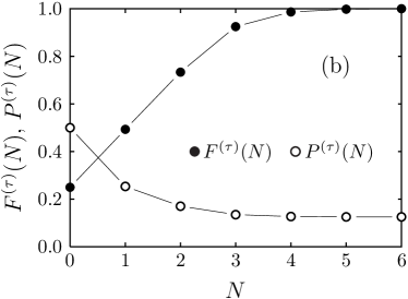
Figure 7: Fidelity $F^{(\tau)}(N)$ and success probability $P^{(\tau)}(N)$ for entanglement purification. The entangled state $|{\Psi^{-}}\rangle_{\text{AB}}$ is extracted from (a) a product state $\varrho_{\text{tot}}=|{\rightarrow}\rangle_{\text{X}}\langle{\rightarrow}|\otimes|{\uparrow}\rangle_{\text{A}}\langle{\uparrow}|\otimes|{\downarrow}\rangle_{\text{B}}\langle{\downarrow}|$ and (b) the thermal state $\varrho_{\text{tot}}\propto e^{-\beta H_{\text{tot}}}$ at temperature $T=(k_{\text{B}}\beta)^{-1}$, through repeated confirmations of the state $|{\rightarrow}\rangle_{\text{X}}$. Parameters are $\Omega=0$, $\tau=0.5\pi\simeq 1.57$ for (a), and $\Omega=0$, $\tau=\zeta/\sqrt{2}\simeq 1.73$, $k_{\text{B}}T=\beta^{-1}=\infty$ for (b), in the unit such that $g=1$, where $\zeta$ is defined in the caption of Fig. 4. For the initial thermal state in (b) with $\Omega=0$, the success probability for the zeroth confirmation is given by $P^{(\tau)}(0)=1/2$ for any set of parameters $(\theta,\varphi,g,T)$, and the final value $P^{(\tau)}(\infty)=[8\cosh^{2}(\beta g/\sqrt{2})]^{-1}$ becomes largest at $k_{\text{B}}T/|g|=(\beta|g|)^{-1}=\infty$.

The extraction of the entangled state $|{\Psi^{-}}\rangle_{\text{AB}}$ is demonstrated in Fig. 7, from a product state $\varrho_{\text{tot}}=|{\rightarrow}\rangle_{\text{X}}\langle{\rightarrow}|\otimes|{\uparrow}\rangle_{\text{A}}\langle{\uparrow}|\otimes|{\downarrow}\rangle_{\text{B}}\langle{\downarrow}|$ and from the thermal equilibrium state $\varrho_{\text{tot}}\propto e^{-\beta H_{\text{tot}}}$ at temperature $T=(k_{\text{B}}\beta)^{-1}$.

VI Concluding Remarks

The examples presented in this article demonstrate how the present purification scheme works, and suggest a few potential applications, even though the analyses are heuristically based and no general “optimization” theory or strategy has been given. Remarkable features of the scheme are summarized as follows. (i) The first point is the simplicity. Many of the other proposed procedures are composed of several steps with different operations, such as rotation, cnot operation, and measurement ref:QuantInfoCompZeilinger ; ref:PurificationBennett . In the present scheme, on the other hand, one has only to repeat one and the same measurement. (ii) Furthermore, the “optimal” success probability is possible in the sense that the target state contained in the initial state is fully extracted. In several other methods ref:QuantInfoCompZeilinger ; ref:PurificationBennett , on the contrary, it decays to zero as the fidelity approaches unity note:Purification . (iii) The number of measurements required for purification is considerably reduced by appropriate choices of parameters, and purification is attainable after only a few steps.

Another point to be stressed is the flexibility. While many of the other schemes ref:QuantInfoCompZeilinger ; ref:PurificationBennett are designed for specific systems, the framework is presented in Sec. II on a general setting, and there are diverse systems and purposes which fit the present scheme. We have already observed, in this article, two different applications on the same idea: initialization and entanglement purification. Additional ideas or slight modifications to the basic scheme would provide us with various methods of state preparation. An interesting extension of the present scheme is for extraction of entanglement between two spatially-separated qubits ref:QuantInfoCompZeilinger ; ref:EntanglementSeparate ; ref:PurificationBennett ; ref:PurificationExperiments , which is often necessary for quantum communication, quantum teleportation, and so on. (The original protocols for entanglement purification ref:QuantInfoCompZeilinger ; ref:PurificationBennett are aimed at this purpose.) It is actually possible and will be reported elsewhere ref:qpfes . One of the other possible extensions is to go beyond a method of extracting quantum state. It would be interesting, for example, if we could find a novel method of transferring quantum state ref:StateTransfer ; ref:StateTransferRev rather than extracting it.

In this article, only qubit systems, i.e., finite-dimensional systems, have been discussed. One has to keep in mind that the condition (12) plays a crucial role in the present purification scheme. If this condition is met, however, it works for infinite-dimensional ones as well. In fact, a harmonic oscillator, which has an infinite number of energy levels, can be purified through the present method, which is explicitly demonstrated in ref:qpf . This also shows the broad range of applicability of the scheme. It is not obvious, however, whether one can purify systems with continuous spectra, since they seem, at first sight, unlikely to satisfy the condition for purification (12), especially the discreteness of the eigenvalues. This point is one of the interesting future subjects, since it would be required in some cases to purify quantum states in the presence of environmental systems, namely, under dissipation and/or dephasing.

The simplicity and the efficiency mentioned above would facilitate practical experimental applications of the present scheme. The flexibility allows one to apply it to various kinds of systems intended for quantum information and computation, such as optical setups ref:PurificationExperiments , ion-trap systems ref:NIST ; ref:Blatt , solid-state quantum computers ref:NEC , and so on. In practice, one should face many unwanted factors, and robustness of the method against them is crucial. In the present scheme, it is often required to tune certain parameters in order to extract a desired pure state, and it is an important subject to clarify how precise the tuning should be and how much error the method suffers from when the parameters are mistuned. It is also a remained issue to explore how ideal projective measurements are realized in actual experiments. Investigations on these points are now in progress.

Appendix A Bound on the Eigenvalues of $V_{\phi}(\tau)$

Let us prove that the eigenvalues $\lambda_{n}$ of the projected time-evolution operator $V_{\phi}(\tau)$ are bounded as in (7).

For an arbitrary state of A, say $|{\psi}\rangle_{\text{A}}$,

$$0 \leq\|V_{\phi}(\tau)|{\psi}\rangle_{\text{A}}\|^{2}$$

$$=\|{}_{\text{X}}\langle{\phi}|e^{-iH_{\text{tot}}\tau}|{\phi}\rangle_{\text{X}}|{\psi}\rangle_{\text{A}}\|^{2}$$

$$\leq\|e^{-iH_{\text{tot}}\tau}|{\phi}\rangle_{\text{X}}|{\psi}\rangle_{\text{A}}\|^{2}$$

$$=1.$$ (49)

Hence, by setting $|{\psi}\rangle_{\text{A}}=|{u_{n}}\rangle_{\text{A}}$ [a right eigenvector of the operator $V_{\phi}(\tau)$] and noting $\|V_{\phi}(\tau)|{u_{n}}\rangle_{\text{A}}\|^{2}=|\lambda_{n}|^{2}$, we obtain the inequality (7). As is clear from this proof, the bound (7) reflects unitarity of the time-evolution operator $e^{-iH_{\text{tot}}\tau}$.

Appendix B A Nondiagonalizable $V_{\phi}(\tau)$ Case

It is assumed in Sec. II that the projected time-evolution operator $V_{\phi}(\tau)$ is diagonalized like (9), but it is not the case if some of its eigenvalues are degenerated. Here we show, however, that the assumption of the diagonalizability is not essential to the purification.

When an eigenvalue $\lambda_{n}$ of the (finite-dimensional) operator $V_{\phi}(\tau)$ is $M_{n}$-fold degenerate, there do not always exist $M_{n}$ linearly independent eigenvectors. This fact spoils the diagonalizability of the operator $V_{\phi}(\tau)$. There exist $d_{n}\,(\leq M_{n})$ linearly independent right eigenvectors $|{u_{n}^{(k)}}\rangle_{\text{A}}$ ($k=1,\ldots,d_{n}$) belonging to the eigenvalue $\lambda_{n}$ ($d_{n}$ is called “dimension of the eigenspace”), and one can find $M_{n}-d_{n}$ linearly independent “generalized eigenvectors” $|{u_{n}^{(k)}}\rangle_{\text{A}}$ ($k=d_{n}+1,\ldots,M_{n}$) which are subjected to the conditions

$$V_{\phi}(\tau)|{u_{n}^{(k)}}\rangle_{\text{A}}=\lambda_{n}|{u_{n}^{(k)}}\rangle_{\text{A}}+|{u_{n}^{(k-1)}}\rangle_{\text{A}}\\ (k=d_{n}+1,\ldots,M_{n})$$ (50)

and linearly independent of the eigenvectors $|{u_{n}^{(k)}}\rangle_{\text{A}}$ ($k=1,\ldots,d_{n}$) ref:Kato . The right vectors $|{u_{n}^{(k)}}\rangle_{\text{A}}$ ($k=1,\ldots,M_{n}$) then form a complete set within the subspace associated with the eigenvalue $\lambda_{n}$, and there exist corresponding left vectors ${}_{\text{A}}\langle{v_{n}^{(k)}}|$ ($k=1,\ldots,M_{n}$), which satisfy the orthonormality

$${}_{\text{A}}\langle{v_{m}^{(k)}}|{u_{n}^{(\ell)}}\rangle_{\text{A}}=\delta_{mn}\delta_{k\ell}$$ (51a)

and completeness conditions

$$\sum_{n}\mathcal{P}_{n}=\openone_{\text{A}},\quad\mathcal{P}_{n}=\sum_{k=1}^{M_{n}}|{u_{n}^{(k)}}\rangle_{\text{A}}\langle{v_{n}^{(k)}}|.$$ (51b)

The operator $V_{\phi}(\tau)$ is now expanded as

$$V_{\phi}(\tau)=\sum_{n}(\lambda_{n}\mathcal{P}_{n}+\mathcal{D}_{n})$$ (52a)

with

$$\mathcal{D}_{n}=\sum_{k=d_{n}+1}^{M_{n}}|{u_{n}^{(k-1)}}\rangle_{\text{A}}\langle{v_{n}^{(k)}}|,$$ (52b)

which is the most general form of spectral decomposition and is called “Jordan canonical form” ref:Kato . Note the relations

$$\mathcal{P}_{m}\mathcal{P}_{n} =\delta_{mn}\mathcal{P}_{n},$$ (53a)

$$\mathcal{D}_{m}\mathcal{P}_{n} =\mathcal{P}_{n}\mathcal{D}_{m}=\mathcal{D}_{m}\delta_{mn},$$ (53b)

$$\mathcal{D}_{m}\mathcal{D}_{n} =0\quad(m\neq n),$$ (53c)

and

$$\mathcal{D}_{n}^{M_{n}-d_{n}+1}=0.$$ (53d)

From the spectral decomposition (52), it is easily deduced that

$$\bm{(}V_{\phi}(\tau)\bm{)}^{N}=\sum_{n}\biggl{(}\lambda_{n}^{N}\mathcal{P}_{n}+\!\!\sum_{r=1}^{\min(N,M_{n}-d_{n})}\!\!\!\!{}_{N}C_{r}\,\lambda_{n}^{N-r}\mathcal{D}_{n}^{r}\biggr{)},$$ (54a)

where

$$\mathcal{D}_{n}^{r}=\sum_{k=d_{n}+r}^{M_{n}}|{u_{n}^{(k-r)}}\rangle_{\text{A}}\langle{v_{n}^{(k)}}|.$$ (54b)

Therefore, if the largest (in magnitude) eigenvalue is unique, which is denoted by $\lambda_{0}$, and nondegenerate (i.e., $M_{0}=1$, $d_{0}=1$, $D_{0}=0$), the single term in the expansion (54a) again dominates asymptotically like (11) (note that ${}_{N}C_{r}\sim N^{r}/r!$ for large $N$), which leads to the same conclusion as (13). The purification does not suffer from degeneracy in the other eigenvalues than the largest (in magnitude) one $\lambda_{0}$. The crucial condition to the purification is (12).

Appendix C Optimization of the Single-Qubit Purification

We show here that the condition (24) together with (27) is the necessary and sufficient condition for the optimal purification with both (12) and (15) for model (18).

First, we try to achieve the upper bound in the inequality (49), i.e., $\|V_{\phi}(\tau)|{\psi}\rangle_{\text{A}}\|=1$, in model (18). If such a state $|{\psi}\rangle_{\text{A}}$ is found and is an eigenstate of the operator $V_{\phi}(\tau)$, say $|{u_{n}}\rangle_{\text{A}}$, we have $|\lambda_{n}|=1$. As is easily seen from (49), the equality holds only when

$${}_{\text{X}}\langle{\phi_{\perp}}|e^{-iH_{\text{tot}}\tau}|{\phi}\rangle_{\text{X}}|{\psi}\rangle_{\text{A}}=0$$ (55)

is satisfied, where $|{\phi_{\perp}}\rangle_{\text{X}}$ is a vector perpendicular to $|{\phi}\rangle_{\text{X}}$ in (23), i.e.,

$$|{\phi_{\perp}}\rangle_{\text{X}}=e^{-i\varphi/2}\sin\frac{\theta}{2}|{\uparrow}\rangle_{\text{X}}-e^{i\varphi/2}\cos\frac{\theta}{2}|{\downarrow}\rangle_{\text{X}}.$$ (56)

Equation (55) means that the operator $V_{\phi}^{\perp}(\tau)\equiv{}_{\text{X}}\langle{\phi_{\perp}}|\times e^{-iH_{\text{tot}}\tau}|{\phi}\rangle_{\text{X}}$ should have a zero eigenvalue, and hence

$$\det V_{\phi}^{\perp}(\tau)=0.$$ (57)

For model (18), the operator $V_{\phi}^{\perp}(\tau)$ reads

$$V_{\phi}^{\perp}(\tau)={} |{\uparrow}\rangle_{\text{A}}\langle{\uparrow}|e^{-i(\Omega_{\text{X}}+\Omega_{\text{A}})\tau}\left[1-e^{i(\Omega_{\text{X}}+\Omega_{\text{A}})\tau/2}\left(\cos\delta\tau+i\frac{\Omega_{\text{X}}-\Omega_{\text{A}}}{2\delta}\sin\delta\tau\right)\right]\sin\frac{\theta}{2}\cos\frac{\theta}{2}$$

$${}-|{\downarrow}\rangle_{\text{A}}\langle{\downarrow}|\left[1-e^{-i(\Omega_{\text{X}}+\Omega_{\text{A}})\tau/2}\left(\cos\delta\tau-i\frac{\Omega_{\text{X}}-\Omega_{\text{A}}}{2\delta}\sin\delta\tau\right)\right]\sin\frac{\theta}{2}\cos\frac{\theta}{2}$$

$${}+i|{\uparrow}\rangle_{\text{A}}\langle{\downarrow}|\frac{g}{\delta}e^{-i\varphi}e^{-i(\Omega_{\text{X}}+\Omega_{\text{A}})\tau/2}\sin\delta\tau\cos^{2}\!\frac{\theta}{2}-i|{\downarrow}\rangle_{\text{A}}\langle{\uparrow}|\frac{g}{\delta}e^{i\varphi}e^{-i(\Omega_{\text{X}}+\Omega_{\text{A}})\tau/2}\sin\delta\tau\sin^{2}\!\frac{\theta}{2},$$ (58)

and

$$\det V_{\phi}^{\perp}(\tau)=-\frac{1}{4}e^{-i(\Omega_{\text{X}}+\Omega_{\text{A}})\tau}\biggl{[}\left|1-e^{i(\Omega_{\text{X}}+\Omega_{\text{A}})\tau/2}\left(\cos\delta\tau+i\frac{\Omega_{\text{X}}-\Omega_{\text{A}}}{2\delta}\sin\delta\tau\right)\right|^{2}+\left(\frac{g}{\delta}\right)^{2}\sin^{2}\!\delta\tau\biggr{]}\sin^{2}\!\theta.$$ (59)

Condition (55), namely (57), is hence reduced to

$$\sin\theta=0$$ (60a)

or

$$\cos\delta\tau=\pm 1\quad\text{and}\quad e^{i(\Omega_{\text{X}}+\Omega_{\text{A}})\tau/2}=\pm 1.$$ (60b)

In the first case (60a), both conditions (12) and (15) are satisfied unless $\delta\tau=n\pi$ ($n=1,2,\ldots$) as is explained around (24)–(27). In the second case (60b), on the other hand, the projected time-evolution operator reads $V_{\phi}(\tau)=\openone_{\text{A}}$ and the eigenvalue $\lambda_{0}=1$ is degenerated, i.e., condition (12) is not fulfilled. Therefore, the necessary and sufficient condition for the optimal purification in model (18) is given by the first choice (60a) [i.e., (24)] with (27).

Appendix D Condition for the Two-Qubit Initialization

We here outline the proof of the necessary and sufficient condition for the optimal two-qubit initialization, Eq. (41), in Sec. IV. What we have to show is how to make the eigenvalues $\lambda_{\pm}$ and $\lambda_{\uparrow\uparrow}$ in (40) all less than unity in magnitude.

The eigenvalues $\lambda_{\pm}$ are the solutions to an eigenvalue equation

$$(\lambda e^{i\Omega\tau})^{2}-2\left(\cos^{2}\!\frac{\bar{g}\tau}{\sqrt{2}}-\sin^{2}\!\chi\sin^{2}\!\frac{\bar{g}\tau}{\sqrt{2}}\right)(\lambda e^{i\Omega\tau})$$

$${}+1-2\cos^{2}\!\chi\sin^{2}\!\frac{\bar{g}\tau}{\sqrt{2}} =0.$$ (61)

We clarify when this equation has a solution whose magnitude is unity. Seeking such a solution, we insert $\lambda=e^{-i\Omega\tau}e^{i\Theta}$ into (61) to obtain the conditions

$$\sin\Theta\left(\cos\Theta-\cos^{2}\!\frac{\bar{g}\tau}{\sqrt{2}}+\sin^{2}\!\chi\sin^{2}\!\frac{\bar{g}\tau}{\sqrt{2}}\right) =0,$$ (62a)

$$\cos\Theta\left(\cos\Theta-\cos^{2}\!\frac{\bar{g}\tau}{\sqrt{2}}+\sin^{2}\!\chi\sin^{2}\!\frac{\bar{g}\tau}{\sqrt{2}}\right)$$

$${}-\cos^{2}\!\chi\sin^{2}\!\frac{\bar{g}\tau}{\sqrt{2}} =0,$$ (62b)

which are reduced to

$$\sin\frac{\bar{g}\tau}{\sqrt{2}}=0\quad \text{and}\quad\cos\Theta=1$$ (63a)

or

$$\cos\frac{\bar{g}\tau}{\sqrt{2}}=0\quad \text{and}\quad\cos\Theta=-1.$$ (63b)

(Note that $\cos\chi\neq 0$ and $\sin\chi\neq 0$, since it is assumed that $g_{\text{XA}},g_{\text{AB}}\neq 0$.) It is easy to see from (40b) that we have $|\lambda_{\uparrow\uparrow}|=1$ when $\sin(\bar{g}\tau/\sqrt{2})=0$, and in summary, the magnitude of one of the eigenvalues $\lambda_{\pm}$ and $\lambda_{\uparrow\uparrow}$ becomes unity only when

$$\sqrt{2}\bar{g}\tau=n\pi\quad(n=1,2,\ldots).$$ (64)

The condition for the initialization in Sec. IV is thus proved to be (41). See also Fig. 4.

Appendix E Condition for the Entanglement Purification

The necessary and sufficient condition (46) for the entanglement purification in Sec. V is proved in a similar manner to that in Appendix D.

The eigenvalues $\lambda_{\pm}$ and $\lambda_{\Phi^{-}}$ under the condition (46a) are the solutions to an eigenvalue equation

$$\left(\kappa-\sin\frac{g\tau}{\sqrt{2}}\right)\left(\kappa-\cos^{2}\!\frac{\theta}{2}\sin\frac{g\tau}{\sqrt{2}}\right)\left(\kappa-\sin^{2}\!\frac{\theta}{2}\sin\frac{g\tau}{\sqrt{2}}\right)$$

$${}+2\sin^{2}\!\frac{\theta}{2}\cos^{2}\!\frac{\theta}{2}\cos^{2}\!\frac{g\tau}{\sqrt{2}}\left(\kappa-\frac{1}{2}\sin\frac{g\tau}{\sqrt{2}}\right)=0$$ (65)

with $\kappa=(1-\lambda)/[2\sin(g\tau/\sqrt{2})]$. Seeking a solution $\lambda$ with unit magnitude, we insert $\lambda=e^{i\Theta}$ into this equation to obtain

$$\sin\Theta\,\biggl{[}2\cos^{2}\!\Theta-\left(3-4\sin^{2}\!\frac{g\tau}{\sqrt{2}}\right)\cos\Theta+1$$

$$\phantom{\sin\Theta\,\biggl{[}}{}-\left(2-\frac{1}{2}\sin^{2}\!\theta\right)\sin^{2}\!\frac{g\tau}{\sqrt{2}}\left(2-\sin^{2}\!\frac{g\tau}{\sqrt{2}}\right)\biggr{]}=0,$$ (66a)

$$\cos\Theta\,\biggl{[}2\cos^{2}\!\Theta-\left(3-4\sin^{2}\!\frac{g\tau}{\sqrt{2}}\right)\cos\Theta$$

$$\phantom{\sin\Theta\,\biggl{[}}{}-\left(2-\frac{1}{2}\sin^{2}\!\theta\right)\sin^{2}\!\frac{g\tau}{\sqrt{2}}\left(2-\sin^{2}\!\frac{g\tau}{\sqrt{2}}\right)\biggr{]}$$

$$\quad\phantom{={}}{}+1-2\sin^{4}\!\frac{g\tau}{\sqrt{2}}-\frac{1}{2}\sin^{2}\!\theta\sin^{2}\!\frac{g\tau}{\sqrt{2}}\left(2-3\sin^{2}\!\frac{g\tau}{\sqrt{2}}\right)$$

$$\quad=0,$$ (66b)

which are reduced to

$$\sin\frac{g\tau}{\sqrt{2}}=0\quad \text{and}\quad\cos\Theta=1$$ (67a)

or

$$\cos\frac{g\tau}{\sqrt{2}}=0\quad \text{and}\quad\cos\Theta=-1.$$ (67b)

Extraction of entanglement is not possible when (67a) or (67b) is satisfied, and therefore, the condition for the entanglement purification in Sec. V is given by (46).

References

(1)
M. A. Nielsen and I. L. Chuang,
Quantum Computation and Quantum Information
(Cambridge University Press, Cambridge, 2000).
(2)The Physics of Quantum Information,
edited by D. Bouwmeester, A. Ekert, and A. Zeilinger
(Springer-Verlag, Heidelberg, 2000).
(3)
K. Vogel, V. M. Akulin, and W. P. Schleich,
Phys. Rev. Lett. 71, 1816 (1993);
A. S. Parkins, P. Marte, P. Zoller, and H. J. Kimble,
ibid.71, 3095 (1993);
B. M. Garraway, B. Sherman, H. Moya-Cessa, P. L. Knight, and
G. Kurizki,
Phys. Rev. A 49, 535 (1994);
C. K. Law and J. H. Eberly,
Phys. Rev. Lett. 76, 1055 (1996);
B. Kneer and C. K. Law,
Phys. Rev. A 57, 2096 (1998),
and references therein.
(4)
J. I. Cirac and P. Zoller,
Phys. Rev. A 50, 2799(R) (1994);
M. Freyberger, P. K. Aravind, M. A. Horne, and A. Shimony,
ibid.53, 1232 (1996);
M. B. Plenio, S. F. Huelga, A. Beige, and P. L. Knight,
ibid.59, 2468 (1999);
J. Hong and H.-W. Lee,
Phys. Rev. Lett. 89, 237901 (2002);
C. Marr, A. Beige, and G. Rempe,
Phys. Rev. A 68, 033817 (2003).
(5)
C. Cabrillo, J. I. Cirac, P. García-Fernández, and P. Zoller,
Phys. Rev. A 59, 1025 (1999);
L.-M. Duan, M. D. Lukin, J. I. Cirac, and P. Zoller,
Nature (London) 414, 413 (2001);
A. Messina, Eur. Phys. J. D 18, 379 (2002);
D. E. Browne and M. B. Plenio,
Phys. Rev. A 67, 012325 (2003);
X.-L. Feng, Z.-M. Zhang, X.-D. Li, S.-Q. Gong, and Z.-Z. Xu,
Phys. Rev. Lett. 90, 217902 (2003);
L.-M. Duan and H. J. Kimble,
ibid.90, 253601 (2003);
D. E. Browne, M. B. Plenio, and S. F. Huelga,
ibid.91, 067901 (2003).
(6)
E. Hagley, X. Maître, G. Nogues, C. Wunderlich, M. Brune,
J. M. Raimond, and S. Haroche,
Phys. Rev. Lett. 79, 1 (1997).
(7)
B. DeMarco, A. Ben-Kish, D. Leibfried, V. Meyer, M. Rowe,
B. M. Jelenković, W. M. Itano, J. Britton, C. Langer,
T. Rosenband, and D. J. Wineland,
Phys. Rev. Lett. 89, 267901 (2002);
A. Ben-Kish, B. DeMarco, V. Meyer, M. Rowe, J. Britton,
W. M. Itano, B. M. Jelenković, C. Langer, D. Leibfried,
T. Rosenband, and D. J. Wineland,
ibid.90, 037902 (2003),
and references therein.
(8)
F. Schmidt-Kaler, H. Häffner, M. Riebe, S. Gulde,
G. P. T. Lancaster, T. Deuschle, C. Becher, C. F. Roos,
J. Eschner, and R. Blatt,
Nature (London) 422, 408 (2003);
F. Schmidt-Kaler, H. Häffner, S. Gulde, M. Riebe,
G. P. T. Lancaster, T. Deuschle, C. Becher, W. Hänsel,
J. Eschner, C. F. Roos, and R. Blatt,
Appl. Phys. B 77, 789 (2003),
and references therein.
(9)
Y. Nakamura, Yu. A. Pashkin, and J. S. Tsai,
Nature (London) 398, 786 (1999);
T. Yamamoto, Yu. A. Pashkin, O. Astafiev, Y. Nakamura, and
J. S. Tsai,
ibid.425, 941 (2003),
and references therein.
(10)
E. Waks, E. Diamanti, and Y. Yamamoto,
quant-ph/0308055 (2003).
(11)
C. H. Bennett, G. Brassard, S. Popescu, B. Schumacher,
J. A. Smolin, and W. K. Wootters,
Phys. Rev. Lett. 76, 722 (1996);
78, 2031(E) (1997);
C. H. Bennett, D. P. DiVincenzo, J. A. Smolin, and
W. K. Wootters,
Phys. Rev. A 54, 3824 (1996).
(12)
T. Yamamoto, M. Koashi, Ş. K. Özdemir, and N. Imoto,
Nature (London) 421, 343 (2003);
Z. Zhao, T. Yang, Y.-A. Chen, A.-N. Zhang, and J.-W. Pan,
Phys. Rev. Lett. 90, 207901 (2003);
A. Vaziri, J.-W. Pan, T. Jennewein, G. Weihs, and A. Zeilinger,
ibid.91, 227902 (2003).
(13)
H. Nakazato, T. Takazawa, and K. Yuasa,
Phys. Rev. Lett. 90, 060401 (2003);
K. Yuasa, H. Nakazato, and T. Takazawa,
J. Phys. Soc. Jpn. 72 Suppl. C, 34 (2003).
(14)
T. Kato, Perturbation Theory for Linear Operators, 2nd ed. (Springer-Verlag, Berlin, 1984).
(15)
For reviews, see
H. Nakazato, M. Namiki, and S. Pascazio,
Int. J. Mod. Phys. B 10, 247 (1996);
D. Home and M. A. B. Whitaker,
Ann. Phys. (N.Y.) 258, 237 (1997);
P. Facchi and S. Pascazio, in Progress in Optics,
edited by E. Wolf (Elsevier, Amsterdam, 2001), Vol. 42, p. 147.
(16)
It should be noted, however, that the time interval in
this scheme is not necessarily small as in the ordinary Zeno
measurements, and the purification (13) is
not due to the quantum Zeno effect. If the ordinary Zeno limit
and ( fixed) ref:QZE
is taken in the present scheme, a quantum Zeno effect appears
yielding the so-called “quantum Zeno dynamics” ref:QZD ,
which is unitary and provides us with a quite different effect
from the one discussed in this article.
(17)
P. Facchi, A. G. Klein, S. Pascazio, and L. S. Schulman,
Phys. Lett. A 257, 232 (1999);
P. Facchi, V. Gorini, G. Marmo, S. Pascazio, and
E. C. G. Sudarshan,
ibid.275, 12 (2000);
P. Facchi, S. Pascazio, A. Scardicchio, and L. S. Schulman,
Phys. Rev. A 65, 012108 (2001);
P. Facchi and S. Pascazio,
Phys. Rev. Lett. 89, 080401 (2002).
(19)
H. Nakazato, M. Unoki, and K. Yuasa,
in Proceedings of ICQI03, Tokyo, 2003 (to be published)
[quant-ph/0403009 (2004)].
(20)
S. Bose, Phys. Rev. Lett. 91, 207901 (2003);
L. Amico, A. Osterloh, F. Plastina, R. Fazio, and G. M. Palma,
Phys. Rev. A 69, 022304 (2004);
V. Subrahmanyam, ibid.69, 034304 (2004);
M. Christandl, N. Datta, A. Ekert, and A. J. Landahl,
quant-ph/0309131 (2003).
(21)
For a review, see
C. H. Bennett and D. P. DiVincenzo,
Nature (London) 404, 247 (2000).