Sequential Probability Ratio Test for the detection of a single electron spin in the OSCAR setup

Abstract

The MRFM device is a powerful setup for manipulating single electron spin in resonance in a magnetic field. However, the real time observation of a resonating spin is still an issue because of the very low SNR of the output signal. This paper investigates the usability and the efficiency of sequential detection schemes (the Sequential Probability Ratio Test) to decrease the required integration time, in comparison to standard fixed time detection schemes.

1 Introduction

Magnetic Resonance Force Microscopy (MRFM) is a promising technique for high-resolution non-destructive spatial imaging. One of the most exciting challenge proposed for MRFM is the observation of single spin in resonance in a magnetic field. Sidles demonstrated the capability of the MRFM for manipulating proton spins [14]. The use of MRFM has since been extended to the observation of electron spins through the use of the OScillating Cantilever-driven Adiabatic Reversal (OSCAR) method [11, 16]. Although micro-size ensembles of electron spins have been detected [21], generating forces as low as $8\times 10^{-10}$ Newton [12], observing a single electron spin in resonance is still an issue because of the weakness of the signal. For the current signal-to-noise ratio (SNR), the required integration time for detection is too long to allow a real-time implementation. The integration time is expected to decrease as technological advances occur improving cantilever sensitivity to single spins and decreasing noise sensitivity. Improvements can also be obtained by making use of advanced signal processing techniques. This is the focus of this paper.

Currently, the presence of one (or several) electron spins in resonance is detected by standard methods of statistical detection. A statistic of an observed sample of fixed length is compared to a threshold. The setting of this threshold splits the space of the statistic into two decision regions. A level of confidence (i.e. a probability of error) is associated to each decision regions. The probability of error decreases when the observation time (the number of data) increases. In order to reach an acceptable level of confidence, the observation time is currently of the order of eight hours.

Sequential analysis was introduced for generic hypothesis testing problems by Wald in 1947 [17] to make decision with a reduced amount of data. This is of great interest for instance in clinical trials where ethical considerations require making decision as soon as possible [2], [15]. The most important feature of Wald’s procedure is that the number of data required to make a decision is a random variable. The borders of the decision regions (and thus the probabilities of error) depend on this random variable through its expected value called the Average Sample Number (ASN).
The first Sequential Probability Ratio Test (SPRT), proposed by Wald was designed to test a simple hypothesis $H_{0}$ versus a simple alternative $H_{1}$. Data are recorded and tested sequentially until a condition on the likelihood ratio to accept one of the hypotheses $H_{i}$ is met. The ASN of the SPRT is smaller than the amount of data required for any fixed sample size test to achieve the same decision error probabilities.

However, the SPRT presents two main drawbacks. Practically speaking, the absence of any upper bound on the stopping time may make the ASN higher than the actual number of data available. Moreover, if there is a mismatch of the $H_{0}$ or $H_{1}$ models and the data, the expected stopping time may be large and, consequently, a sequential procedure may not improve on a fixed sample size procedure [4]. Much work has been done to avoid such shortcomings. The main feature of the modified SPRT proposed in the literature is to introduce a bound on the stopping time [1], [2]. This led to a class of test called Truncated Sequential Probability Ratio Test (TSPRT). When performing a TSPRT, a decision is taken at a given sample size $N$ even if neither of the stopping conditions has been met before $N$. Such modification increases the error probabilities. Another way to deal with the uncertainty and mismatch on the hypotheses is to take into account a priori information by means of the Bayes formalism [10]. Many monographs have been published since the early book of Wald. Most of them adopt a probabilistic approach [15], [19], by focussing on the error probability aspect. Wijsman’s approach in [20] is slightly different; since it is common to consider sequential procedures by means of Brownian Motion, his analysis of sequential test (and more generally sequential procedures) relies on elements of the theory of diffusion which makes it an original introduction to sequential analysis.

The aim of this paper is to investigate the usability of the SPRT in the specific problem of detecting a single electron spin in the OSCAR setting. We focus on two sequential tests of the variance of the observed signal, namely a $\chi^{2}$ and a Fisher-F test. The main contribution of this paper is to derive the exact expression of the ASN of the $\chi^{2}$ test and a low snr development of the ASN of the Fisher-F test. These expressions allow a comparison to the number of data required to perform the corresponding fixed sample size tests. A procedure is also proposed to perform an experimental validation of this comparison in the case of the $\chi^{2}$ test.

2 Data processing and fixed sample size detection scheme

We address the problem of detecting an electron in resonance in the OSCAR experiment. Before performing the detection procedure, the data are pre-processed in order to enhance the performances of the detector. In this section we briefly describe the OSCAR setup and the associated signal processing.

2.1 Data models

2.1.1 General outline

Figure 1: The OSCAR setup.

In the OSCAR experiment, presented in Figure 1, a sample is embedded in a Radio-Frequency (RF) magnetic field $B_{1}$. If the RF-field frequency matches the Larmor frequency of an electron in the sample, the electron spin is in magnetic resonance [5]. A cantilever with a ferromagnet on its tip is settled close to the sample. The cantilever is forced into mechanical oscillations at frequency $\omega_{0}$ which induces an oscillating magnetic field. As a consequence, the spin polarity of any free electron in the resonant slice of the device is forced to reverse synchronously with the ferromagnet motion. Moreover, in the so-called interrupted OSCAR experiment, the RF-field is turned off every $T_{skip}$ seconds so that the spin polarity is reversed periodically. The successive steps of the pre-processing are presented on Figure 2.

Figure 2: The pre-processing scheme.

Output of the interferometer.

The spin reversal induces a slight change in the cantilever stiffness. The electron spin can thus be detected by observing a shift $\delta\omega_{0}$ in the natural frequency of the cantilever. The motion of the cantilever is measured by a laser interferometer. When a spin is resonating in the resonant slice, the output of the interferometer is a frequency-modulated signal of form:

$$z(t)=A\cos\{\omega_{0}t+\int_{0}^{t}s(u)du+\phi\},$$ (1)

where $A$ is the amplitude of the oscillation, $\phi$ is a random phase and $s(u)$ is a square-wave of period $2T_{skip}$ and magnitude $\delta\omega_{0}$. When no electron in the resonant slice is resonating, there is no shift in the natural frequency and $z(t)=A\cos\{\omega_{0}t+\phi\}$.

Spin relaxation.

The spin can spontaneously go out of alignment with the magnetic field. This phenomenon called spin relaxation is not fully understood. One model for the effect of spin relaxation is that when relaxation occurs, the polarity of the spin changes. This causes $\lambda$ random flips per second. The relaxation phenomenon is taken into account in the modelling of the output of the cantilever by means of a random telegraph signal. In continuous time, the number of random flips is considered as following a Poisson distribution with rate $\lambda T$ where $T$ is the duration of the observation. The equivalent discrete-time model is a $2$-state Markov chain. If the transition probabilities $p$ between states are equal, then $p=1-T_{s}\lambda$ where $T_{s}$ is the sampling rate. Other models include random walks on the sphere and random walks on the interval. See [16] for a review of these different models.

Frequency demodulation and sampling.

The square-wave is estimated by demodulating the signal with a frequency lock-in device. Then the output of the frequency lock-in is sampled. The frequency lock-in can be seen as a frequency estimator whose variance induces an additive noise. Considerations on the dynamical system describing the spin-cantilever interaction lead to a natural alternative which makes use of an efficient estimator of the square-wave related to the MUSIC algorithm [6].

Output of the correlator and filtering.

In order to remove the deterministic square-wave, the discrete signal is correlated to a reference square-wave of period $2T_{skip}$ resulting in a baseband signal with the natural frequency $\omega_{0}$ removed. This is the so-called in phase filtering of the output of the frequency estimator.
The signal-to-noise ratio is increased by filtering the sampled data over the pass-band of the spin signal with a low-pass filter defined by the recursive relation:

$$x_{n}=\alpha x_{n-1}+\frac{1-\alpha}{2}(z_{n}+z_{n-1}),$$ (2)

where $z_{n}$ is the input of the filter and $x_{n}$, the output. The cut-off frequency $\omega_{c}$ of this recursive filter is set by parameter $\alpha$:

$$\alpha=\frac{1-\sin\{\omega_{c}\}}{\cos\{\omega_{c}\}}.$$ (3)

This filtering induces a coloration of the embedding noise. In order to consider that the assumption on independence of the data samples is valid, the output of the filter is subsampled at the rate $2\pi/\omega_{c}$.

2.1.2 SNR estimation

A noise-alone reference can be generated by correlating the demodulated signal with a version of the reference square-wave phase-shifted by $90^{o}$. This is the so-called quadrature filtering. The ratio of the energies of the output of the in-phase channel to the output of the quadrature channel provides an estimate of the signal-to-noise ratio. Under an i.i.d. Gaussian assumption on the sampled demodulated cantilever signal, this ratio is by definition a Fisher-F random variable. It will be used as the test statistic for the so-called Fisher-F test that we describe in this paper.

Figure 3: The SNR estimation scheme.

2.2 The energy detector.

The single spin detection problem can be formulated as making a decision between the two hypotheses:

$$\left\{\begin{array}[]{ll}H_{0}:&x_{n}=\nu_{n},\\ H_{1}:&x_{n}=d_{n}+\nu_{n},\end{array}\right.$$ (4)

where $d_{n}$ is a random signal with RMS amplitude $\sigma_{d}$ and intensity $\lambda$ and $\nu_{n}$ is a white Gaussian noise with zero-mean and variance $\sigma^{2}_{\nu}$. When the SNR $\sigma^{2}_{d}/\sigma^{2}_{\nu}$ is sufficiently small we can consider $x_{n}$ as a Gaussian random variable with zero-mean and variance $\sigma^{2}_{\nu}+\sigma^{2}_{d}$ under $H_{1}$. In this case the single spin test consists in deciding:

$$\left\{\begin{array}[]{ll}H_{0}:&x_{n}\sim{\cal N}(0,\sigma^{2}_{\nu}),\\ H_{1}:&x_{n}\sim{\cal N}(0,\sigma^{2}_{\nu}+\sigma^{2}_{d}),\end{array}\right.$$ (5)

where $X\sim Y$ means that the random variable $X$ has the same PDF as the random variable $Y$. The detection procedure is applied to the energy $E^{(N)}_{x}=\sum_{n=1}^{N}x_{n}^{2}$. The energy $E^{(N)}_{x}$ under both hypotheses are sums of $N$ independent identically distributed squared Gaussian variables. They are random variables following $\chi^{2}$ distributions with $N$ degrees of freedom and scale parameter equal to the variance of the Gaussian variables. The hypotheses (5) can be equivalently formulated as:

$$\left\{\begin{array}[]{ll}H_{0}:&E^{(N)}_{x}\sim\sigma^{2}_{\nu}\chi^{2}_{N},\\ H_{1}:&E^{(N)}_{x}\sim(\sigma^{2}_{\nu}+\sigma^{2}_{d})\chi^{2}_{N}.\end{array}\right.$$ (6)

The Probability Density Function (PDF) of a $\sigma^{2}\chi^{2}_{df}$ random variable with scale parameter $\sigma^{2}$ and $df$ degrees of freedom is of the form:

$$f_{\sigma^{2}\chi^{2}_{df}}(x)=\frac{1}{(2\sigma^{2})^{df/2}\Gamma(df/2)}x^{df/2-1}e^{-x/2\sigma^{2}},$$ (7)

where $\Gamma(u)$ is the gamma function.

2.3 The Fisher-F test

When $\sigma^{2}_{\nu}$ is unknown, the $\chi^{2}$-test derived from the energy detector can no longer be applied. An alternative detection procedure is based on the ratio of the energies of the quadrature and in-phase channel components. Under the hypotheses given by (4), the models for the in-phase channel component $x^{i}_{n}$ and for the quadrature component channel $x^{q}_{n}$ are:

$$\left\{\begin{array}[]{llcl}H_{0}:&x^{i}_{n}\sim{\cal N}(0,\sigma^{2}_{\nu})&\mbox{and}&x^{q}_{n}\sim{\cal N}(0,\sigma^{2}_{\nu}),\\ H_{1}:&x^{i}_{n}\sim{\cal N}(0,\sigma^{2}_{\nu}+\sigma^{2}_{d})&\mbox{and}&x^{q}_{n}\sim{\cal N}(0,\sigma^{2}_{\nu}).\end{array}\right.$$ (8)

The detection procedure is applied to the ratio $R^{(N)}_{x}$ of the energies:

$$R^{(N)}_{x}=E^{(N)}_{x^{i}}/E^{(N)}_{x^{q}}.$$ (9)

As already mentioned in the case of the energy detector, under the Gaussian assumption on $x$ the energies are $\chi^{2}$ distributed with $N$ degrees of freedom and scale parameter equal to the variance of the Gaussian variables. The ratio of the $\chi^{2}$ variables is a Fisher-F random variable denoted $\sigma^{2}{\cal F}(N,N)$ with $N$ and $N$ degrees of freedom and scale parameter $\sigma^{2}$ equal to the ratio of the scale parameters of the $\chi^{2}$ variables. Thus the Fisher-F detector can be formulated as testing the two hypotheses:

$$\left\{\begin{array}[]{ll}H_{0}:&R^{(N)}_{x}\sim{\cal F}(N,N),\\ H_{1}:&R^{(N)}_{x}\sim(1+snr){\cal F}(N,N),\end{array}\right.$$ (10)

where the random variable $\sigma^{2}{\cal F}(df,df)$ has a Fisher-F PDF of the form:

$$f_{\sigma^{2}{\cal F}(df,df)}(x)=\frac{1}{\sigma^{2}}\frac{\Gamma(df)}{\Gamma(df/2)^{2}}\frac{(x/\sigma^{2})^{df/2-1}}{(1+x/\sigma^{2})^{df}}.$$ (11)

2.4 Likelihood Ratio Tests

2.4.1 Generality

Given a random variable ${\bf X}$ having a PDF $f_{\theta}({\bf x})$ defined by the parameter $\theta$, the likelihood function $l(\theta;{\bf x})$ of a sample ${\bf x}$ of ${\bf X}$ is defined as $l(\theta;{\bf x})=f_{\theta}({\bf x})$. The Likelihood Ratio Test (LRT) consists in testing simple hypothesis $H_{0}$ under which $X$ follows $f_{0}({\bf x})=f_{\theta_{0}}({\bf x})$ versus the simple alternative $H_{1}$ under which $X$ follows $f_{1}({\bf x})=f_{\theta_{1}}({\bf x})$ by setting a threshold $\tau$ on the likelihood ratio statistic:

$$\lambda({\bf x})=\frac{f_{1}({\bf x})}{f_{0}({\bf x})}.$$ (12)

If $\lambda({\bf x})>\tau$ hypothesis $H_{0}$ is rejected and vice-versa. The notation:

$$\begin{array}[]{ccc}&H_{1}&\\ \lambda({\bf x})&\gtrless&\tau,\\ &H_{0}&\end{array}$$ (13)

is often adopted to evoke the LRT.

Error probabilities of the test

The LRT is intended at taking a decision given a finite sample of a random variable. The performance of a test is evaluated by the decision error probabilities. The probability of miss $P_{mis}$ (also called the probability of error of first kind) is the probability of deciding $H_{0}$ when $H_{1}$ is true and the probability of false alarm $P_{fa}$ (also called the probability of error of second kind) is the probability of deciding $H_{1}$ when $H_{0}$ is true. The threshold $\tau$ determines the error probabilities. An ideal test would require to choose $\tau$ such that both error probabilities tend to zero. Unfortunately the probability of miss increases when the probability of false alarm decreases. The user has to decide which one of the errors is preferable. However, the LRT is often referred as the optimal test in the sense that for a given $P_{fa}$, the LRT provides the smallest $P_{mis}$.

Decision regions

The LRT splits the sample space into two exclusive regions of acceptance of $H_{0}$ or $H_{1}$. For fixed sample size $N$, the boundary between the decision regions depends on the probabilities of error through the setting of $\tau$ and $N$. Thus, given a sample size $N$ and a threshold $\tau$, $P_{mis}$ and $P_{fa}$ are uniquely defined.

2.4.2 The Energy detector

For the LRT involving the likelihood function (7) of the energy $E^{(N)}_{x}$, the test statistic (12) takes the form:

$$\lambda^{(N)}({\bf x})=\left(\frac{1}{1+snr}\right)^{N/2}\mbox{exp}\{\frac{1}{2\sigma_{\nu}^{2}}\frac{snr}{1+snr}E^{(N)}_{x}\},$$ (14)

where for sake of simplicity in the notations, the dependence on $E^{(N)}_{x}$ is replaced by a dependence on ${\bf x}=x_{1},\ldots,x_{N}$ and $snr=\frac{\sigma^{2}_{d}}{\sigma^{2}_{\nu}}$. It is often more convenient to test the log-likelihood $\Lambda^{(N)}({\bf x})$ of the data:

$$\Lambda^{(N)}({\bf x})=\log\{\lambda^{(N)}({\bf x})\}=\frac{snr}{1+snr}\frac{1}{2\sigma^{2}_{\nu}}E^{(N)}_{x}-\frac{N}{2}\log\{1+snr\}.$$ (15)

One can see that the log-likelihood ratio statistic depends on the energy $E^{(N)}_{x}$ through parameters $snr$ and $\sigma^{2}_{\nu}$ which are common to both hypotheses. Hence, when testing two normal distributions with zero mean and different known variances, the energy detector is equivalent to the LRT.

2.4.3 The Fisher-F Ratio detector

The log-likelihood ratio of the energy ratio $R^{(N)}_{x}$ is defined from expression (11) of the Fisher-F PDF by:

$$\Lambda^{(N)}(x)=\frac{N}{2}\log\{1+snr\}+N\log\{1+x\}-N\log\{1+snr+x\}.$$ (16)

Unlike the log-likelihood ratio (15) involved in the energy detector, this test statistic depends only on the signal-to-noise ratio $snr$. Knowledge on the noise variance is not required to implement the Fisher-F test. This is the reason why this test is currently preferred in the OSCAR experiment.

2.4.4 Required sample number

Expressions (6) and (10) show that the parameter of interest for discriminating between the hypotheses is the scale parameter $\sigma^{2}_{i}$. In both cases, the scale parameters are such that $\sigma^{2}_{1}=(1+snr)\sigma^{2}_{0}$. The cumulative distribution functions $F_{i}(\tau)=\int_{0}^{\tau}f_{i}(u)\mbox{d}u$ of the $\chi^{2}$ and the Fisher-F random variables for $i=0,1$ satisfy the relation:

$$F_{1}(\tau)=F_{0}(\frac{\tau}{1+snr}).$$ (17)

The probability of miss can thus be expressed as a function of the probability of detection, parameterized by $snr$, and the sample size $N$. The required number of samples can be evaluated for a given test with a given strength $(P_{fa},P_{mis})=(\alpha,\beta)$ by constraining $P_{fa}$, and choosing $N$ such that $P_{mis}$ is reached.

3 Sequential Detection Procedures

Unlike fixed sample size procedures, the sample size required in a sequential procedure is a random number called the sample number. The Average Sample Number (ASN) can be dramatically smaller than the corresponding sample size $N$ required to perform a fixed sample size test of at least same strength $(\alpha,\beta)$ [15, 17]. The Relative Sample Efficiency (RSE) of a sequential procedure with respect to a fixed sample size procedure is the ratio $N/\mbox{ASN}$.

3.1 Sequential Probability Ratio Test

A fixed sample size test splits the sample space into two decision regions. A sequential procedure splits the sample space into three regions; the region of acceptance of $H_{0}$, the region of acceptance of $H_{1}$, and the continuation region where the decision is postponed and another sample is acquired. More specifically, suppose a decision has to be taken from the likelihood ratio statistic $\lambda^{(n)}$ computed from the $n$ first available samples $x_{1},x_{2},\ldots,x_{n}$. Two constants $A$ and $B$ are chosen such that $A>B$ and the SPRT is defined as follows:

$$\left\{\begin{array}[]{ll}\lambda^{(n)}\leq B:&\mbox{accept }H_{0},\\ B<\lambda^{(n)}<A:&\mbox{postpone the decision},\\ \lambda^{(n)}\geq A:&\mbox{accept }H_{1}\end{array}\right.$$ (18)

The thresholds $A$ and $B$ define the boundaries between the three decision regions. The stopping time or sample number $N_{s}$ is defined by:

$$N_{s}=\min\{N_{0},N_{1}\},$$ (19)

where $N_{0}$ (resp. $N_{1}$) is the first time the likelihood ratio statistic crosses the boundary $A$ (resp. $B$). The probability that such a test terminates is one. Wald and Wolfowitz have shown that among all the sequential test, the SPRT provides the smallest ASN under both hypotheses [18]. For a desired strength $(\alpha,\beta)$ of test, the boundaries are set by the Wald’s approximations [9, 17]:

$$A&=\frac{1-\beta}{\alpha}\\ B=\frac{\beta}{1-\alpha}.$$ (20)

These approximations hold for small error probabilities, typically smaller than $0.05$.

Operating Characteristic and Average Sample Number function

The design of the SPRT assumes that the parameters $\theta_{i}$ defining the hypotheses are known. The behavior of the test strongly depends on this assumption. In particular, the ASN can dramatically increase if the true parameter $\theta$ does not match the hypotheses. The Operating Characteristic $L(\theta)$ is the probability of accepting $H_{0}$ when the true parameter is $\theta$. In particular, $L(\theta_{0})=1-P_{fa}$ and $L(\theta_{1})=P_{mis}$. The operating characteristic is an efficient tool for evaluating the performances of the test under a model mismatch.
Wald shows that the operating characteristic of the SPRT can be approximated by:

$$L(\theta)\approx\frac{A^{h}-1}{A^{h}-B^{h}},$$ (21)

where $h$ is solution of the integral equation:

$$\int_{-\infty}^{+\infty}\left(\frac{f(x,\theta_{1})}{f(x,\theta_{0})}\right)^{h}f(x,\theta)dx=1.$$ (22)

One can see from this equation that $h$ depends on the true parameter $\theta$. For instance the solutions in the cases $\theta=\theta_{0}$ and $\theta=\theta_{1}$ can be computed by noting that $f(x,\theta)$ is a PDF:

$$\left\{\begin{array}[]{lcc}h=1&\mbox{if}&\theta=\theta_{0},\\ h=-1&\mbox{if}&\theta=\theta_{1}.\end{array}\right.$$ (23)

In general, $h$ cannot be evaluated explicitly for every $\theta$ and one has to approximate it numerically. A possible approach suggested by Wald consists of solving equation (22) by finding the value of $\theta$ for which the equation is verified by a given value of $h$ [17].
Wald makes use of the operating characteristic (21) and of the approximations (20) to derive an approximation to the ASN $E\{N|\theta\}$ required to stop the SPRT when the true parameter is $\theta$:

$$E\{N|\theta\}=\frac{L(\theta)\log\{B\}+(1-L(\theta))\log\{A\}}{E\{\Lambda(x)|\theta\}},$$ (24)

where $\Lambda(x)=\Lambda^{(1)}(x)$. Unlike the operating characteristic, the ASN depends on the model through the expected value of the log-likelihood ratio.

3.2 The Approximation of the Log-Likelihood Ratio Statistic as a Brownian Motion

Most of the properties of the SPRT are model-independent. In particular, the statistical behavior of the SPRT can be studied by approximating the sequential log-likelihood ratio statistic as a Brownian Motion [15].

3.2.1 The Brownian Motion

Definition of a Brownian Motion.

A Brownian Motion (also called a Wiener process) $W(t)\sim{\cal B}{\cal M}(\mu,\sigma^{2})$, $0\leqslant t<\infty$ with drift $\mu$ and variance $\sigma^{2}$ is a random process such that:

• $W(0)=0$;

• $W(t)-W(s)\sim{\cal N}(\mu(t-s),\sigma^{2}(t-s))$, for all $0\leqslant s<t<\infty$;

• for all $0\leqslant s_{1}<t_{1}<s_{2}<t_{2}<\infty$, $W(t)-W(s)\sim{\cal N}(\mu(t-s),\sigma^{2}(t-s))$, the random variables $W(t_{1})-W(s_{1})$ and $W(t_{2})-W(s_{2})$ are independent;

• $W(t)$, $0\leqslant t<\infty$ is a continuous function of $t$.

If the mean and variance of $\Lambda^{(N)}({\bf x})$ are linear functions of the sample size $N$, the log-likelihood ratio can be considered as the sampled Brownian Motion $W(t)=W(NT_{s})=\Lambda^{(N)}({\bf x})\sim{\cal B}{\cal M}(\mu,\sigma^{2})$. Then by equating the first and second moments of $\Lambda^{(N)}$ under $H_{0}$ and $H_{1}$, one can compute the drift $\mu_{i}$ and the variance $\sigma^{2}_{i}$ under hypothesis $H_{i}$. The test can then be formulated under a new model:

$$\left\{\begin{array}[]{ll}H_{0}:&W(t)\sim{\cal B}{\cal M}(\mu_{0},\sigma^{2}_{0}),\\ H_{1}:&W(t)\sim{\cal B}{\cal M}(\mu_{1},\sigma^{2}_{1}),\end{array}\right.$$ (25)

where $\mu_{i}$ and $\sigma_{i}$ are parameters characterizing the performance of the test procedure.
The drifts and variances are derived from the first and second order moments of the test statistic. Thus the approximation of the sequential likelihood ratio statistic as a sampled version of a Brownian Motion is valid up to the second order moment. A drawback of such an approximation is that the skewness of the distribution is not taken into account. This leads to an overestimation of the expected value of the stopping time in many situation. This phenomenon is known as the overshooting [20]. The overshooting phenomenon has been evaluated numerically for some tests [15].

3.2.2 Truncated SPRT and prediction of the sample number

In many applications, the number of samples available is limited. After a given time, a decision has to be made even though the sample still spans the neutral region. Define the truncated Sequential Probability Ratio Test (TSPRT) with stopping rules:

$$\left\{\begin{array}[]{rcl}T_{0}&=&\min\{\inf\{n:\Lambda^{(n)}\leqslant\log\{A\}\},N\},\\ T_{1}&=&\min\{\inf\{n:\Lambda^{(n)}\geqslant\log\{B\}\},N\},\end{array}\right.$$ (26)

where $N$ is the maximum practicable sample size. Under both hypotheses, if $T_{i}<N$ then the estimated stopping time is $N_{i}=T_{i}$, else, thanks to the definition of Brownian Motion, one can predict what should be the stopping time if additional samples were to be taken. Indeed, $N_{i}$ is such that

$$W(N_{i}T_{s})-W(NT_{s})\sim{\cal N}(\mu(N_{i}-N)T_{s},\sigma^{2}(N_{i}-N)T_{s}).$$ (27)

By noting that $W(NT_{s})=\Lambda^{(N)}$ and $W(N_{i}T_{s})=\log\{A\}$ under $H_{0}$ and $W(N_{i}T_{s})=\log\{B\}$ under $H_{1}$ one can express:

$$\left\{\begin{array}[]{rcl}N_{0}&=&N+\frac{1}{\mu_{0}}(\log\{A\}-\Lambda^{(N)}),\\ N_{1}&=&N+\frac{1}{\mu_{1}}(\log\{B\}-\Lambda^{(N)}).\end{array}\right.$$ (28)

On Figure 4 are presented the histograms of the estimated ASN $E_{0}\{N_{0}\}$ and $E_{1}\{N_{1}\}$ for lengths $N=1000$ and $N=5000$ for the SPRT based on the energy statistic described in next section. One hundred trials have been performed. The strength of the test is $P_{fa}=_{mis}=0.02$. The signal-to-noise ratio is $-20dB$ before filtering. It has been chosen such that for each trial, $1000<N_{0},N_{1}<5000$ with high probability. Thus for each trial, when $N=1000$ (dashed lines) the sample number has to be predicted and when $N=5000$ (plain line), it can be observed. The tail of the true histogram is heavier than for the predicted histogram. Indeed, the prediction scheme is based on the approximation of the likelihood ratio as a Brownian Motion. The distribution of the predicted sample number is closer to a Gaussian distribution. The consequence is a reduction of the skewness. Thus like for the approximation (24) proposed by Wald, the ASN is slightly under-estimated by approximating the likelihood ratio sequence as a Brownian motion.

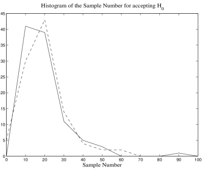
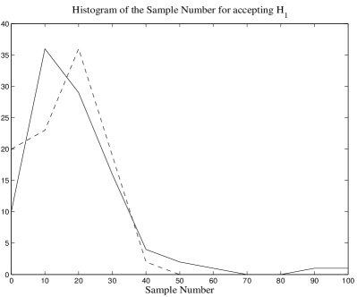
Figure 4: Experimental evaluation of the accuracy of the prediction of the required sample number. The histograms of the prediction (dashed line) are superimposed to the histograms of the actual sample number (plain lines).

3.3 SPRT based on the energy statistic

In the case of $\chi^{2}$ (or Gamma) distributions, Bartholomew [3] and Phatarfod [13] have proposed specific formulations of the procedure for application of a sequential test to analysis of the arrival time of a random event. These works concern distributions which differ under the null hypothesis and the alternative by the number of degrees freedom. We are concerned with distributions which present the same number of degrees of freedom, namely, the sample number.
The expected value and variance of a $\sigma^{2}\chi^{2}_{N}$ random variable are:

$$E\{\sigma^{2}\chi^{2}_{N}\}=N\sigma^{2}.$$ (29)

$$Var\{\sigma^{2}\chi^{2}_{N}\}=2N(\sigma^{2})^{2},$$ (30)

so, under the hypotheses (6), the test statistic (15) can be approximated by the following Brownian motion:

$$\left\{\begin{array}[]{ll}H_{0}:&W(t)\sim{\cal B}{\cal M}(\frac{snr}{2(1+snr)}-\frac{1}{2}\log\{1+snr\},\frac{snr^{2}}{2(1+snr)^{2}}),\\ H_{1}:&W(t)\sim{\cal B}{\cal M}(\frac{snr}{2}-\frac{1}{2}\log\{1+snr\},\frac{1}{2(1+snr)^{2}}),\end{array}\right.$$ (31)

Figure 5 displays the ratio of the ASN to the number of sample required for the fixed sample LRT with same error probabilities. The ASN have been estimated as the average of the sample numbers computed from $100$ trials of $20000$ points. After filtering the sub-sampling reduces the sample size to $N=250$. When the test failed to stop before $N$, the prediction procedure described in section 3.2 was applied. The number of samples required for the fixed sample size test has been computed numerically from the known expression of the error probabilities as described in section 2.4.2.
At higher SNR, the number of samples required for both the sequential test and the standard test are of the order of the unit, so the computed ratios cannot be considered as reliable. At low SNR, the RSE is around two.

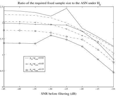
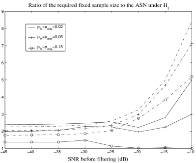
Figure 5: Evaluation of the $\chi^{2}$ test: RSE of the energy detector under $H_{0}$ (left) and $H_{1}$ (right). The dashed-dotted lines are the theoretical RSE.

The RSE increases when the error probabilities decrease. This makes the SPRT particularly attractive when the level of confidence put on the decision is to be high.
The ratios predicted from Wald’s approximation (24) of the ASN are superimposed to the experimental ratios. At low error probabilities, one can see that Wald’s expression over-estimates the true ASN. This phenomenon is associated with the skewness of the PDF (highlighted by Figure 4) [15, 19]. It is of interest to notice that when the error probabilities increase (see the case $P_{fa}=P_{mis}=0.15$), approximation  (24) no longer holds and the ASN tends to be under-estimated. However, the improvement is still significant. Above this value, there is no gain in using a sequential test.

3.4 SPRT based on the Fisher-F statistic

Jackson [7] and Jennison [8] have derived exact values of the operating curve and ASN for the sequential Fisher test when the parameter of interest is the mean of a normal population. Like Bartholomew in [3] and Phatarfod in [13], Jennison makes use of Cox’s theorem to transform the observation and apply the test to a new statistic which is independent on the number of degrees of freedom. Such approach cannot be adopted in our case as the parameter of interest is the variance of the normal population.
An exact expression of the expected value of the log-likelihood (16) has yet to be derived. We propose in the Appendix a derivation of an approximation that holds at low snr. One can see with expressions (49) that the expected value of the log-likelihood is not a linear function of the number of data. Thus, the approximation as a Brownian Motion is not valid for the Fisher-F test statistic. Consequently, the sample size prediction procedure does not hold and the experimental evaluation of the ASN cannot be performed. On Figure 6 is presented the theoretical ratio of the ASN under $H_{1}$ to the number of samples required for the fixed sample size test of same strength at low snr ($-30dB$ before filtering).
When the error probabilities are smaller than $0.06$, the SPRT significantly reduces the required sample size. A strength of $\alpha=\beta=0.02$ can be achieved by a fixed sample size test if the sample size is of the order of $10^{7}$. The use of the SPRT allows a reduction of the order of $10^{6}$ data samples. When the error probabilities are above $0.06$ the ratio is smaller than $1$, which is due to the fact that the Wald’s approximation is not reliable for large error probabilities.
The right-hand side of Figure 6 displays the ASN of the Fisher-F test to the ASN of the $\chi^{2}$ test ratio computed from expression (24) and approximation (49) under $H_{0}$ and $H_{1}$. As far as Wald’s approximation holds, one can see from expression (24) that this ratio is independent of the error probabilities. At low signal-to-noise ratio, the ASN of the Fisher-F test is $4$ times the ASN of the $\chi^{2}$ test.

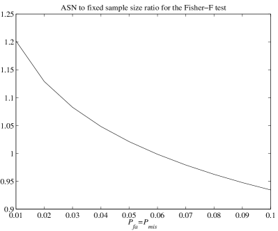
Figure 6: Evaluation of the Fisher-F test: RSE of the Fisher-F test under $H_{1}$ for various error probabilities (left). The snr before filtering is $-30dB$. Ratio of the ASN of the Fisher-F test to the ASN of the $\chi^{2}$ test (right) uner $H_{0}$ (dashed line) and under $H_{1}$ (plain line).

4 Conclusion

The advantages of Sequential Probability Ratio Tests (SPRT) for detection in a $\chi^{2}$ and Fisher-F model has been investigated. Evaluation of the relative sample efficiency of the SPRT with respect to the corresponding fixed sample size test has been computed on simulation data.
For these test, it was experimentally verified that a gain of $50\%$ in the required integration time can be expected at low SNR (below $-30dB$). The appealing feature of the proposed model is that the test statistic can be written in a closed form which avoid making use of approximations.
A similar study has been performed to evaluate the efficiency of a Fisher-F type test based on the ratio of the energies of the in-phase and quadrature channel outputs. This test requires only the knowledge of the signal-to-noise ratio and can be performed whatever the noise variance. The consequence is an increase in the ASN of he Fisher-F test in comparison to the $\chi^{2}$ test. At low error probabilities, the ASN is still smaller than the number of samples required to perform a fixed sample size Fisher-F test of same strength.
Another direction required for application to the OSCAR experiment is the evaluation of SPRT performances for unknown bandwidth of the spin signal. This will allow SPRT to be developed for the filter bank implementation of the OSCAR experimental apparatus.

Appendix

Expected value of the statistic of the Fisher test

The log-likelihood ratio of the Fisher-F test is of form:

$$\Lambda^{(N)}(x)=\frac{N}{2}\log\{1+snr\}+N\log\{1+x\}-N\log\{1+snr+x\}.$$ (32)

The expansion into Taylor series of this function around $snr=0$ provides the approximation for small $snr$:

$$\Lambda^{(N)}(x)=\frac{N}{2}\log\{1+snr\}+N\sum_{m=1}^{M}(-1)^{m}\frac{snr^{m}}{m(1+x)^{m}}+o(M).$$ (33)

Thus the expected values of the likelihood ratio under both hypotheses involves the terms $E_{i}\{1/(1+x)^{m}\}$.

Computation of $E_{0}\{\frac{1}{(1+x)^{m}}\}$.

Under $H_{0}$ these terms are written:

$$E_{0}\{\frac{1}{(1+x)^{m}}\} = \int_{0}^{+\infty}\frac{1}{(1+x)^{m}}\frac{\Gamma(N)}{\Gamma(N/2)^{2}}\frac{x^{N/2-1}}{(1+x)^{N}}dx,$$ (34)

$$= \frac{\Gamma(N)}{\Gamma(N/2)^{2}}\int_{0}^{+\infty}\frac{1}{(1+x)^{m}}\frac{x^{N/2-1}}{(1+x)^{N}}dx.$$ (35)

After the change of variable $y=\log(1+x)$, this term takes the form:

$$E_{0}\{\frac{1}{(1+x)^{m}}\} = \frac{\Gamma(N)}{\Gamma(N/2)^{2}}\int_{0}^{+\infty}\mbox{e}^{-(N+m-1)y}(\mbox{e}^{y}-1)^{N/2-1}dy,$$ (36)

$$= \frac{\Gamma(N)}{\Gamma(N/2)^{2}}A_{m}(N,1),$$

where the integral $A_{m}(N,b)$ is defined by:

$$A_{m}(N,b)=\int_{0}^{+\infty}\mbox{e}^{-(N+m-b)y}(\mbox{e}^{y}-1)^{N/2-b}dy.$$ (37)

An integration by parts involving the functions:

$$f(y) = \mbox{e}^{-(N+m-b+1)y},$$

$$g(y) = \frac{1}{N/2-b+1}(\mbox{e}^{y}-1)^{n/2-b+1},$$

show that under the condition $b\leq n/2$, $A_{m}(n,b)$ satisfies the recursive equation:

$$A_{m}(N,b)=\alpha_{m}(N,b)A_{m}(N,b-1),$$ (38)

where $\alpha(N,b)=\frac{N+m-b+1}{N/2-b+1}$. This equation leads to the relation:

$$\forall b,c A_{m}(N,c)= \frac{A_{m}(N,b)}{\prod_{k=c+1}^{b}\alpha_{m}(N,k)}.$$ (39)

By noting that for the case $b=N/2$, $A_{m}(N,N/2)=2/(N+2m)$, expression (39) takes the form:

$$\forall c A_{m}(N,c)= \frac{2/N}{\prod_{k=c+1}^{N/2}\alpha(N,k)}.$$ (40)

This equality holds for even values of $N$. It is asymptotically true for the odd values of $N$. The denominator can be expressed in terms of Gamma functions:

$$\prod_{k=c+1}^{N/2}\alpha(N,k)=\frac{\Gamma(N+m-c+1)}{\Gamma(N/2-c+1)\Gamma(N/2+m+1)},$$

and the integral $A_{m}(N,b)$ takes the form:

$$A_{m}(N,b)=\frac{\Gamma(N/2-b+1)\Gamma(N/2+m)}{\Gamma(N+m-b+1)}.$$ (41)

By injecting this expression into (36), the expected value of $1/(1+x)^{m}$ under $H_{0}$ is finally written:

$$E_{0}\{\frac{1}{(1+x)^{m}}\}=\frac{\Gamma(N)\Gamma(N/2+m)}{\Gamma(N/2)\Gamma(N+m)}.$$ (42)

Computation of $E_{1}\{\frac{1}{(1+x)^{m}}\}$.

The expected value of $1/(1+x)^{m}$ under $H_{1}$ is of form:

$$E_{1}\{\frac{1}{(1+x)^{m}}\}=\frac{\Gamma(N)}{\Gamma(N/2)^{2}}\int_{0}^{+\infty}\frac{1}{(1+x)^{m}}\frac{1}{1+snr}\frac{(x/(1+snr)^{N/2-1}}{(1+x/(1+snr))^{N}}dx.$$ (43)

After the change of variable $y=x/(1+snr)$ this expression takes the form:

$$E_{1}\{\frac{1}{(1+x)^{m}}\}=\frac{\Gamma(N)}{\Gamma(N/2)^{2}}\int_{0}^{+\infty}h(y,snr)\frac{y^{N/2-1}}{(1+y)^{N}}dx.$$ (44)

where $h(y,snr)=\frac{1}{(1+y(1+snr))^{m}}$. An expansion of $h(y,snr)$ into Taylor series around $snr=0$:

$$h(y,snr)=\sum_{k=0}^{K}(-1)^{k}\frac{\Gamma(m+k)}{\Gamma(m)}\frac{(snry)^{k}}{k!(1+y)^{m+k}}+o(K),$$ (45)

leads to the expression:

$$E_{1}\{\frac{1}{(1+x)^{m}}\}\approx\frac{\Gamma(N)}{\Gamma(N/2)^{2}}\sum_{k=0}^{K}(-1)^{k}\frac{\Gamma(m+k)}{\Gamma(m)}\frac{snr^{k}}{k!}\int_{0}^{+\infty}\frac{y^{k}}{(1+y)^{m+k}}\frac{y^{N/2-1}}{(1+y)^{N}}dy,$$ (46)

where one can recognize the integrals $A_{m}(N,1-k)$ previously defined. Finally, the expected value of $1/(1+x)^{m}$ under $H_{1}$ takes the form:

$$E_{1}\{\frac{1}{(1+x)^{m}}\}\approx\frac{\Gamma(N)}{\Gamma(N/2)^{2}}\sum_{k=0}^{K}(-1)^{k}\frac{\Gamma(m+k)}{\Gamma(m)}\frac{snr^{k}}{k!}A_{m}(N,1-k),$$ (47)

The expected values of the likelihood ratio statistic take finally the forms:

$$E_{0}\{\Lambda^{(N)}(x)\} \approx \frac{N}{2}\log\{1+snr\}+N\frac{\Gamma(N)}{\Gamma(N/2)^{2}}\sum_{m=1}^{M}(-1)^{m}\frac{snr^{m}}{m}A_{m}(N,1),$$ (48)

$$E_{1}\{\Lambda^{(N)}(x)\} \approx \frac{N}{2}\log\{1+snr\}$$ (49)

$$+ N\frac{\Gamma(N)}{\Gamma(N/2)^{2}}\sum_{m=1}^{M}\sum_{k=0}^{K}(-1)^{m+k}\frac{\Gamma(m+k)}{\Gamma(m)}\frac{snr^{m+k}}{k!m}A_{m}(N,1-k).$$

References

- [1] T. W. Anderson. A modification of the sequential probability ratio test to reduce the sample size. Ann. Math. Stat., 31:165–197, March 1960.
- [2] P. Armitage. Restricted sequential procedures. Biometrika, 44:9–26, June 1957.
- [3] D.J. Bartholomew. A sequential test for randomness of intervals. Journal of the Royal Statistical Society, (1):95–103, 1956.
- [4] R E. Bechhofer. A Note on the Limiting Relative Efficiency of the Wald Sequential Probability Ratio Test. Journal of the American Statistical Association, 55(292):660–663, December 1960.
- [5] C. Cohen-Tannoudji, B. Diu, and F. Laloë. Quantum Mechanics. Hermann and Wiley & Son, 1977.
- [6] C. Hory, M. Ting, and A. O. Hero. Frequency tracking procedure derived from a dynamical system analysis. In Proceedings of SSP’03, pages 185–188, St-Louis, Mo, USA, October 2003.
- [7] J. E. Jackson and R. A. Bradley. Sequential and Tests. The Annals of Mathematical Statistics, 32(4):1063–1077, December 1961.
- [8] C. Jennison and B. W. Turnbull. Exact calculations for sequential and F tests. Biometrika, 78(1):133–141, 1991.
- [9] N. L. Johnson. Sequential Analysis: A Survey. Journal of the Royal Statistical Society, (3):372–411, 1961.
- [10] J. Kiefer and L. Weiss. Some properties of Generalized Sequential Probability Ratio Tests. Ann. Math. Stat., 28(1):57–75, March 1957.
- [11] H. J. Mamin, R. Budakian, B. W. Chui, and D. Rugar. Detection and manipulation of statistical polarization in small ensembles. Physical Review Letters, 91, November 2003.
- [12] H. J. Mamin and D. Rugar. Sub-attonewton force detection at milikelvin temperatures. Applied Physics Letters, 79(20):3358–3360, November 2001.
- [13] R. M. Phatarfod. A sequential test for gamma distribution, 1971.
- [14] J. A. Sidles. Nondestructive detection of single-proton magnetic resonance. Applied Physics Letters, 58(24):2854–2856, June 1991.
- [15] D. Siegmund. Sequential Analysis. Springer-Verlag, 1985.
- [16] M. Ting, A. O. Hero, D. Rugar ad J. F. Fessler, and C.-Y-Yip. Electron spin detection in the frequency domain under the interrupted Oscillating Cantilever-driven Adiabatic Reversal (ioscar) Protocol. submitted to IEEE trans. on signal proc., 2003.
- [17] A. Wald. Sequential Analysis. Wiley and Sons, New-York, 1947.
- [18] A. Wald and J. Wolfowitz. Optimum character of the sequential probability ratio test. Ann. Math. Stat., 19:326–339, 1948.
- [19] G. B. Wetherill and K. D. Glazebrook. Sequential Methods in Statistics. Chapman and Hall, third edition, 1986.
- [20] R. A. Wijsman. Stopping Times: Termination, Moments, Distribution. In B. K. Ghosh and P. K. Sen, editors, Handbook of Sequential Analysis, pages 67–119. Marcel Dekker, 1991.
- [21] O. Züger, S. T. Hoen, C. S. Yannoni, and D. Rugar. Three dimensional imaging with a nuclear magnetic resonance force microscope. Journal of Applied Physics, 79(4):1881–1884, February 1996.