Solitons Formed by Dark-State Polaritons in Electromagnetic Induced Transparency

Abstract

We show the possible stable soliton generation for the dark-state polaritons (DSPs) in an electromagnetic induced transparency (EIT) medium composed of $\Lambda$-type atoms. Whether the solitons are dark or bright can be controlled by the coupling field intensity and the one photon detuning of the probe field. The velocity, spatial and time widths of the solitons can also be adjusted by the coupling light.

PACS numbers: 42.65.Tg, 42.50.Gy, 42.65.Wi

The intriguing problem to find new quantum systems whose wave functions can form solitons and to study their novel dynamical properties always attracts considerable interests. The well-known examples include the Ginzburg-Pitaevskii-Gross equation 1 ; 2 in Bose-Einstein Condensate(BEC) and the Maxwell-Bloch equation 3 in nonlinear electric medium, where there exists soliton solutions that respectively describe the properties of wave functions of the atomic condensate and the electric field. A natural question then may be asked: in an interacting system of atoms and electromagnetic field, if we treat them as a total system, can the coupled matter-photon system also form a soliton? An important concrete example may be the light storage in the electromagnetic induced transparency (EIT)4 medium which, in recent years, received much attention due to its potential applications in the field of quantum information science.

In fact since the technique of resonant enhancement of the index of refraction without absorption was proposed 5 and many accompanying striking phenomena was observed 6 ; 7 ; 8 ; 9 ; 10 ; 11 , the light storage with the technique of EIT has been an exciting research field in current literature, especially after the ”dark-state polaritons” (DSPs) theory was proposed by Fleischhauer and Lukin et al.12 ; 13 based on a field theory reformulation of the adiabatic approximation14 . DSP is a new quantum field which is the superpositions of the electric field amplitude $\varepsilon(z,t)$ and atom coherence $\rho_{cb}$ between two lower levels of the $\Lambda$ type atoms, and it describes the total system of the electric field and collective atomic state. In linear theory where the one-photon detuning of the probe pulse is zero, the quantum state of the polaritons can be mapped from the electric field state into the collective atomic excitation without change when the coupling laser was adiabatically turned off12 ; 13 , which implies that DSP is really an elegant description of the total system.

The paper will discuss the nonlinear properties of the DSPs and prove that the motion of the DSPs satisfies a (1+1)dimensional nonlinear Schrödinger equation (NLSE) that has possible stable soliton solutions in an electromagnetic induced transparency (EIT) medium composed of $\Lambda$ type atoms. Note that the soliton is not formed by the probe pulse or atom coherence alone, but by the total state function of them. This is different from the familiar conventional ones15 which are formed by the wave function of a single physical system. The coupling field intensity, along with the one photon detuning of the probe field, is shown to decide whether the solitons are dark or bright and other important parameters, like the time width and the velocity of the solitons.

We consider the quasi 1-dimensional system composed of three-level $\Lambda$-type configuration atoms with energy levels assumed to be $E_{a}>E_{c}>E_{b}$. A coherent probe field with positive frequency part of the electric field $E_{p}^{(+)}(z,t)$ couples the transition between the ground state $|b\!\!>$ and the excited state $|a\!\!>$. $\Delta=\omega_{ab}-\omega$ is the small one-photon detuning between the carrier frequency $\omega$ and the atomic transition frequency $\omega_{ab}$. The stable state $|c\!\!>$ is coupled to $|a\!\!>$ via a coherent coupling field with Rabi-frequency $\Omega$. We assume the coupling pulse is much stronger than the probe one and its frequency is $\nu=\omega_{ac}$. Due to the small intensity of the probe field, we expand the density matrix in the following form:

$$\rho_{\mu\nu}=\rho^{(0)}_{\mu\nu}+\rho^{(1)}_{\mu\nu}+\rho^{(2)}_{\mu\nu}+\rho^{(3)}_{\mu\nu}+...$$ (1)

where $\mu,\nu=a,b$. The quantities $\rho^{(1)}_{\mu\nu}$ is of the same order of smallness as intensity of the probe pulse, the $\rho^{(2)}_{\mu\nu}$ is of the second order of the smallness, and so on. To analyze the nonlinearity of the susceptibility of the probe light, we calculate the density matrix element $\rho_{ab}$ to the third order. Together with the relation: $\wp_{ab}n_{a}(\rho^{(1)}_{ab}+\rho^{(3)}_{ab})=\epsilon_{0}(\chi^{(1)}(\omega)+\chi^{(3)}(\omega)|\varepsilon|^{2})\varepsilon$, where $\varepsilon$ is the dimensionless slowly varying amplitude of the probe pulse $E_{p}(z,t)$ and $n_{a}$ being the atom density, the susceptibility ($\chi\approx\chi^{(1)}+3\chi^{(3)}|\varepsilon|^{2}$) is then given by

$$\chi(\omega)\approx-\frac{2g^{2}N\Delta}{\Omega^{2}\omega}-\frac{6g^{4}N\Delta|\varepsilon|^{2}}{\Omega^{4}(1+\frac{-\Delta^{2}+i\gamma_{ab}\Delta}{\Omega^{2}})\omega}$$ (2)

where $\gamma_{\mu\nu}$ ($\mu,\nu=a,b,c$) is the transverse decay rate between levels $\mu$ and $\nu$ and here they satisfy: $\gamma_{cb},\gamma_{ca}\ll\Omega$; $g=\wp_{ab}\sqrt{\frac{\omega}{2\hbar\epsilon_{0}V}}$, and N is the effective total atoms in the quantum volume V. The susceptibility is related to the refractive index through $n=\sqrt{1+\chi_{(}\omega)}$, then the wave vector of the probe pulse can be approximately calculated by

$$k\approx k_{ab}+\frac{3}{2}k_{ab}\chi^{(3)}|\varepsilon|^{2}+\beta_{1}(\omega-\omega_{ab})+\beta_{2}(\omega-\omega_{ab})^{2}$$ (3)

where $\beta_{1}=\frac{\partial{k}}{\partial{\omega}}|_{\omega=\omega_{ab}}=1/(c\cos^{2}\theta(t))$ is the inverse of the group velocity of the probe pulse, $\beta_{2}=\frac{1}{2}\frac{\partial^{2}{k}}{\partial^{2}{\omega}}|_{\omega=\omega_{ab}}=-\tan^{4}\theta/(\omega_{0}c)$ and $k_{ab}=\omega_{ab}/c$. The mixing angle $\theta$ is defined via $\tan\theta(t)=g\sqrt{N}/\Omega(t)$, which is a sufficiently slowly time-dependent function. Assuming that the wave vector of the probe pulse has a narrow spreading around the central value $k_{0}$, from the formula (3) the frequency of the probe pulse can be expanded around $k_{0}$ in the following form:

$$\omega\approx\omega_{0}-\frac{3}{2}k_{0}V_{g}\chi^{(3)}|\varepsilon|^{2}+V_{g}(k-k_{0})-\beta_{2}V^{3}_{g}(k-k_{0})^{2}$$ (4)

where $V_{g}=c\cos^{2}\theta$ and $\omega_{0}=k_{0}c$ are respectively the group velocity and central frequency of the probe pulse. So the dispersion equation of probe field $E_{p}(z,t)$ can be approximately given by

$$i\frac{\partial{E_{p}(z,t)}}{\partial{t}}= (\omega_{0}-\frac{3}{2}k_{0}V_{g}\chi^{(3)}|\varepsilon|^{2})E_{p}(z,t) +V_{g}(\frac{1}{i}\frac{\partial}{\partial{z}}-k_{0})E_{p}(z,t)$$ (5)

$$-\beta_{2}V_{g}^{3}(\frac{1}{i}\frac{\partial}{\partial{z}}-k_{0})^{2}E_{p}(z,t)$$

In above derivation the varying of Rabi frequency $\Omega$ with time is ignored. In fact, the time-dependent character of $\Omega$ brings a reduction/enhancement of the amplitude $\varepsilon(z,t)$ by a contribution $\frac{\dot{\alpha}}{2(1+\alpha)}\varepsilon$ 13 ; 16 to the motion equation of the probe pulse during the Raman adiabatic passage, where the group index $\alpha=g^{2}N/\Omega^{2}$ and $\dot{\alpha}=d\alpha/dt$. Consequently the propagation equation of the probe pulse in the EIT medium is

$$ik_{0}(\frac{1}{V_{g}}\frac{\partial}{\partial{t}}+\frac{\partial}{\partial{z}}+\frac{\dot{\alpha}}{2c})\varepsilon(z,t)= k_{0}\beta_{2}V^{2}_{g}\frac{\partial^{2}}{\partial{z}^{2}}\varepsilon(z,t) -\eta(\omega_{0})|\varepsilon|^{2}\varepsilon(z,t)$$ (6)

where $\eta(\omega_{0})=\frac{3\omega^{2}_{0}\chi^{(3)}}{2c^{2}}$ and $c$ is the vacuum light speed.

As is known that the propagation of the electromagnetic pulse in an EIT medium can be easily understood in terms of new quantum fields, i.e., polariton-like fields, which are superpositions of the dimensionless electric field amplitude $\varepsilon(z,t)$ and the atom coherence $\rho_{cb}$. The dark-state polaritons and bright-state polaritons(BSP) here are defined by17

$$\Psi(z,t)=\cos\theta(t)\varepsilon(z,t)-\sin\theta(t)\sqrt{N}\rho_{cb}(z,t)\exp(i(k_{0}-k_{c})z)$$ (7)

$$\Phi(z,t)=\sin\theta(t)\varepsilon(z,t)+\cos\theta(t)\sqrt{N}\rho_{cb}(z,t)\exp(i(k_{0}-k_{c})z)$$ (8)

where $k_{c}$ is the wave-vector of the coupling field in $z$ direction, the mixing angle $\theta$ is a function of time, while the electric field $\varepsilon(z,t)$ and atom coherence $\rho_{cb}$ are functions of time and z-axis coordinate. Together with the formula(6), by a straightforward calculation one can derive the propagation equation of the DSPs:

$$ik_{0}(\frac{1}{V_{g}}\frac{\partial}{\partial{t}}+\frac{\partial}{\partial{z}})\Psi(z,t)-k_{0}\beta_{2}V^{2}_{g}\frac{\partial^{2}}{\partial{z}^{2}}\Psi(z,t)$$

$$=ik_{0}\frac{1}{V_{g}}\dot{\theta}\Phi-\frac{ik_{0}}{\cos^{2}\theta}\sin\theta(\frac{\partial\tan\theta\varepsilon}{\partial t}+\sqrt{N}\frac{\partial\widetilde{\rho}_{cb}}{\partial t})-ik_{0}\tan\theta\frac{\partial}{\partial{z}}\Phi$$

$$+k_{0}\beta_{2}V^{2}_{g}\tan\theta\frac{\partial^{2}}{\partial{z}^{2}}\Phi-\eta(\omega_{0})|\varepsilon|^{2}\varepsilon(z,t)$$ (9)

where $\widetilde{\rho}_{cb}=\rho_{cb}(z,t)\exp(i(k_{0}-k_{c})z)$ and $\dot{\theta}=d\theta/dt$. The motion equation of BSPs satisfies 17 :

$$\Phi=\frac{\sin\theta}{g^{2}N}\Bigl{(}\frac{\partial}{\partial t}+\gamma_{ba}+i\Delta\Bigr{)}\Bigl{(}\tan\theta\Bigr{)}\Bigl{[}(\frac{\partial}{\partial t}+i\Delta)(\sin\theta\,\Psi-\cos\theta\,\Phi)+g\sqrt{N}\varepsilon\rho_{ca}\Bigr{]}+i\frac{\sin\theta}{g\sqrt{N}}F_{ba}.$$ (10)

where $F_{ba}$ is Langevin noise term which will be omitted in the following derivation; and the density matrix $|\rho_{ca}|\sim|\varepsilon|^{2}$ and $|\rho_{ca}|\approx|\frac{g\Delta\varepsilon}{\Omega^{2}}\rho_{cb}|\ll|\rho_{cb}|$ due to the weak probe field and low atomic excitation. By introducing the adiabatic parameter $\epsilon\equiv(g\sqrt{N}T)^{-1}$ with $T$ being a characteristic time 12 ; 17 , we find in the lowest order adiabatic theory that, $|\Phi(z,t)|\sim|\frac{g\varepsilon}{\Omega}\rho_{ca}|\approx\frac{|g\Delta|}{|\Omega|^{2}}|\frac{g\varepsilon}{\Omega}|^{2}|\cos\theta\Psi|$ for the ultraslow light case. It is clear that when $|\Omega|^{2}\geq|g\Delta|$ or $|\Omega|^{2}\sim|g\Delta|$, one has $|\Phi|\ll|\cos\theta\Psi|$ (since the control field is much stronger than the probe one, i.e., $|\Omega|^{2}\gg|g\varepsilon|^{2}$). The typical values of these parameters in ultraslow light case are 13 ; 15 $\Omega=1.0\times 10^{6\sim 8}s^{-1}$, $\Delta=1.0\times 10^{7}s^{-1}$ $g\sqrt{N}=5.0\times 10^{12}s^{-1}$ and $g=2.0\times 10^{6}$, from which we find $\cos\theta\sim 10^{-(4\sim 5)}$ and $|\Omega|^{2}\sim|g\Delta|$ and then $|\Phi|\sim|\frac{g\varepsilon}{\Omega}|^{2}|\cos\theta\Psi|\ll|\cos\theta\Psi|$. Hence one can approximately obtain $\varepsilon(z,t)\approx\cos\theta(t)\Psi(z,t)$, $\sqrt{N}\widetilde{\rho}_{cb}\approx-\sin\theta(t)\Psi(z,t)$ and $\Phi\approx 0$. Substituting these results into the formula (Solitons Formed by Dark-State Polaritons in Electromagnetic Induced Transparency) yields

$$ik\frac{\partial}{\partial{t}}\Psi(\xi,t)+\frac{\partial^{2}}{\partial{\xi}^{2}}\Psi(\xi,t)=-C_{n}|\Psi|^{2}\Psi(\xi,t)$$ (11)

where $k=k_{0}/(V_{g}\sin^{4}\theta)$, the slowly varying nonlinear coefficient $C_{n}=\eta(\omega_{0})\cot^{2}\theta\csc^{2}\theta$, and $\xi=z-\int^{t}_{t_{0}}{d\tau V_{g}}$ is the coordinate in the rest frame of the probe pulse. This is a (1+1)-dimensional nonlinear Schrödinger equation (NLSE), which has a bright (dark) soliton solution when Re($\eta(\omega_{0}))>0$ (Re($\eta(\omega_{0}))<0$). As is known, the NLSE with slowly varying coefficients can be solved with perturbation theory 18 . The substitution $t^{\prime}=\int^{t}_{0}dt/k$, $\Psi(\xi,t)=\frac{\Psi^{\prime}(\xi,t^{\prime})}{\sqrt{|C_{n}/2|}}$ transforms Eq.(11) into standard form with perturbation $i\dot{\theta}\frac{1}{2C_{n}}\frac{\partial{C_{n}}}{\partial{\theta}}\Psi$ 18 ; 19 :

$$i\frac{\partial}{\partial{t^{\prime}}}\Psi^{\prime}(\xi,t^{\prime})+\frac{\partial^{2}}{\partial{\xi}^{2}}\Psi^{\prime}(\xi,t^{\prime})+2|\Psi^{\prime}|^{2}\Psi^{\prime}(\xi,t^{\prime})=i\dot{\theta}P(\Psi^{\prime})$$ (12)

where$P(\Psi^{\prime})=\frac{1}{2C_{n}}\frac{\partial{C_{n}}}{\partial{\theta}}\Psi^{\prime}(\xi,t^{\prime})$. In the ultraslow light case $V_{g}\ll{c}$, we have $P(\Psi)\approx\tan\theta\Psi$. Then, when $\Delta<0$ and $\gamma^{2}_{ab}\ll\Delta^{2}<\Omega^{2}$, with a perturbation theory and one can obtain the fundamental bright soliton: 18 ; 20

$$\Psi^{\prime}_{b}=Asech(\sqrt{2}{A\xi})\exp(i\int_{t_{0}}^{t^{\prime}}{d\tau{2A^{2}}})$$ (13)

where $A=A_{0}\cos\theta(0)/\cos\theta(t)$ and $A_{0}$ is a constant related to the initial condition. Then

$$\Psi_{b}=Msech(\sqrt{|C_{n}|}{M\xi})\exp(i\int_{t_{0}}^{t}{d\tau{M^{2}}}|C_{n}|/k)$$ (14)

or

$$\Psi_{b}=Msech({\sqrt{|C_{n}|}M(z-\int^{t}_{t_{0}}V_{g}d\tau)})\exp(i\int_{t_{0}}^{t}{d\tau M^{2}|C_{n}|}/k)$$ (15)

where $M=\frac{A_{0}\cos\theta(0)}{|C_{n}(t)/2|^{1/2}\cos\theta(t)}$ is the maximum amplitude of the soliton. From the formula (13) and (14) one can easily find the spatial width of the soliton $\Delta\xi=ln(2+\sqrt{3})|Nc(\Omega^{2}-\Delta^{2})/(6k_{0}\Omega^{2}{M^{2}(t)}\Delta)|^{1/2}\cos\theta(t)\propto\Omega(t)$, which can be easily controlled by the coupling light. When the Rabi frequency is adiabatically reduced, the spatial width narrows according to $\Delta\xi(t)=\Delta\xi(0)\Omega(t)/\Omega(0)$. Likewise we obtain the time width of the soliton $\tau_{FWHM}=ln(2+\sqrt{3})|N(\Omega^{2}-\Delta^{2})/(6k_{0}\Omega^{2}{M^{2}(t)}\Delta)\cos^{2}\theta(t)|^{1/2}\propto 1/\Omega(t)$, which is inversely proportional to the Rabi-frequency of the coupling light. When $\Omega$ is adiabatically reduced, the time width broadens according to $\tau_{FWHM}(t)=\tau_{FWHM1}(0)\Omega(0)/\Omega(t)$. The result that time and spatial widths can be controlled by the coupling light is an important observation for the properties of the bright solitions formed by DSPs. To give a numerical estimate of the spatial width of the soliton, we assume 13 ; 15 the Rabi frequency of the coupling pulse $\Omega=1.0\times 10^{8}s^{-1}$,one-photon detuning $\Delta=1.0\times 10^{7}s^{-1}$, $g\sqrt{N}=5.0\times 10^{12}s^{-1}$, $N=1.0\times 10^{13}$, $A_{0}\cos\theta(0)\approx 0.1$, and $\omega_{0}=2.0\times 10^{15}s^{-1}$, the spatial width can be then calculated $\Delta\xi\approx 2.63\times 10^{-1}mm$. This estimation indicates that this interesting result may be observable under present experimental techniques (the length of the EIT medium used in present experiment is about several centimeters21 ). By choosing $E_{0}=M(0)$, $L=1/A_{0}$, and $\tau=g^{2}N/(\Omega^{2}(0)A_{0}c)$ as units to normalize the amplitude of the DSPs, coordinate $z$ and time $t$, respectively, the amplitude of the fundamental bright soliton can be plotted in Fig.1.

The derivation of the above result is under the condition Re($\eta(\omega_{0}))>0$. However, when the coupling field intensity is adiabatically reduced to $\Omega^{2}<\Delta^{2}$ while even $\Omega^{2}\sim|g\Delta|$ with $\Delta<0$, the nonlinear coefficient $C_{n}$ becomes a negative. Meanwhile the NLSE supports a dark soliton solution, the amplitude of which is a hyperbolic tangent function. The time or spatial width of the dark solitons has the same form as that of the bright ones. On the other hand, if we initially set a positive one-photon detuning, i.e. $\Delta>0$, the DSPs can also form dark solitons (for the case $\Omega^{2}>\Delta^{2}$) and bright ones (for the case $\Omega^{2}<\Delta^{2}$).

It is noteworthy that in our formulation we have ignored the transverse decay rate $\gamma_{ab}$ which can lead to a contribution $-i\delta|\Psi^{\prime}|^{2}\Psi(z,t)$ to the right-hand side (RHS) of eq.(12), where the coefficient $\delta\propto$ Im$(C_{n})/|C_{n}|\approx\gamma_{ab}|\Delta|/\bigr{[}(\Omega^{2}-\Delta^{2})^{2}+\gamma_{ab}^{2}\Delta^{2}\bigr{]}^{1/2}$ represents a nonlinear loss (absorption) and instability for the propagation of NS solitons. For present purpose, when $|\Omega^{2}-\Delta^{2}|\gg|\gamma_{ab}\Delta|$, the effect of nonlinear absorption can be ignored. The velocity of the solitons we discussed above is just the group velocity of the probe pulse and it can also be conveniently controlled by the coupling pulse. Another interesting issue is that we may extrapolate the idea in this paper to other interacting systems such as a passive medium 22 or a Tonks gas 23 , and we may even introduce a new technique for quantum memory with solitons formed by total state function of quantum memories (QMEs) and quantum carriers (QCAs). Due to the strong stability of solitons, quantum information may be elegantly stored and released against some environmental noise or external field disturbances in this technique.

In conclusion we have shown that the dark-state polaritons in an EIT medium can form the possible stable solitons, and whether the solitons are dark or bright is dependent on the coupling field intensity and the one-photon detuning of the probe field. Note that the kind of solitons are formed by the total wave function of two different physical systems, i.e., the electromagnetic field and collective atomic excitations (spin waves). The velocity, time and spatial widths of the solitons are also shown to be adjustable by the coupling light. Of course, these results are derived for a weak probe field and low atomic excitation, i.e., the atomic density is approximately be treated as constant, and the more interesting case with a varying density is not studied at present. This challenging issue, together with the evolution process from bright solitons to dark ones, deserves further studies in our future works.

We thank Zhengxin Liu , Guimei Jiang , Xu Cao and Xin Liu for their helpful discussions. This work is in part supported by NSF of China under Grant No.10304020. One of the authors (H. J.) is also supported by China Postdoctoral Science Fund and Shanghai Postdoc Research Plan.

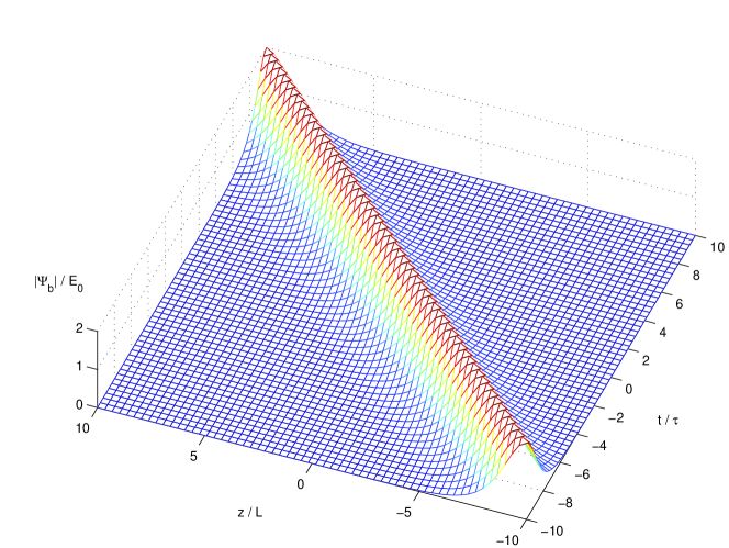
Figure 1: The amplitude of the fundamental bright soliton formed by the DSPs with dimensionless variables. The normalized factors are $E_{0}=M(0)$, $L=1/A_{0}$, and $\tau=g^{2}N/(\Omega^{2}(0)A_{0}c)$ that represent the units of the amplitude of the DSPs, coordinate $z$ and time $t$.

References

(1) V.L.Ginzburg and L.P.Pitaevskii, Sov.Phys.
-JETP,7:858(1958); L.P.Pitaevskii, Sov.Phys.
-JETP,13:451(1961)
(2) E.P.Gross, Nuovo Cimento, 20,454(1961)
(3) L.D.Landau, and E.M.Lifshitz, Electrodynamics of
Continuons Media(Oxford,1984)
(4) M.O.Scully and M.S.Zubairy, Quantum Optics (Cambridge University Press, Cambridge, 1999)
(5) M.O.Scully, Phys.Rev.Lett, 67,1855(1991)
(6) L.V.Hau et al., Nature (London) 397,594(1999)
(7) M.M.Kash et al., Phys.Rev.Lett.82, 5229(1999)
(8) C.Liu, Z.Dutton, C.H.Behroozi, and L.V.Hau et al., Nature (London) 397,490(2001)
(9) S.E.Harris, J.E.Field, and A.Kasapi, Phys.Rev.A, 46,R29(1992)
(10) M.D.Lukin et al. Phys.Rev.Lett 79,2959(1997)
(11) M.Kash et al. Phys.Rev.Lett 82,5229(1999)
(12) M.Fleischhauer and M.D.Lukin, Phys.Rev.Lett. 84, 5094 (2000)
(13) M.Fleischhauer and M.D.Lukin, Phys.Rev.A 65,022314(2002)
(14) C.P.Sun, Y.Li, and X.F.Liu, Phys.Rev.Lett. 91,147903(2003)
(15) Y.S.Kivshar et al., Phys.Rep. 298,81(1998) J.Denschlag et al., Science, 287,97(2000);
T. Hong, Phys.Rev.Lett 90,183901(2003)
(16) U.Leonhardt, arXiv:gr-qc/0108085(2002)
(17) C.Mewes and M.Fleischhauer, Phys. Rev. A 66, 033820 (2002)
(18) Y.S.Kivshar and B.A.Malomed, Rev.Mod.Phys.61,4(1989)
(19) V.I.Karpman and E.M.Maslov, Phys.Fluids 25,1686(1982)
(20) J.P.Keener and D.W.Mclaughlin, Phys.Rev.A 16,777(1977)
(21) D.F.Phillips, A.Fleischhauer et al., Phys.Rev.Lett.86,783(2001)
(22) M. Bajcsy, A. S. Zibrov and M. D. Lukin, Nature 426, 638 (2003)
(23) B. Paredes, et al., Nature 429, 277 (2004)