Quantum process tomography of a controlled-not gate

Abstract

We demonstrate complete characterization of a two-qubit entangling process – a linear optics controlled-not gate operating with coincident detection – by quantum process tomography. We use a maximum-likelihood estimation to convert the experimental data into a physical process matrix. The process matrix allows accurate prediction of the operation of the gate for arbitrary input states and calculation of gate performance measures such as the average gate fidelity, average purity and entangling capability of our gate, which are 0.90, 0.83 and 0.73 respectively.

Quantum information science offers the potential for major advances such as quantum computing Nielsen and Chuang (2000) and quantum communication Gisin et al. (2002), as well as many other quantum technologies Dowling and Milburn (2003). Two-qubit entangling gates, such as the controlled-not (cnot), are fundamental elements in the archetypal quantum computer Nielsen and Chuang (2000). A promising proposal for achieving scalable quantum computing is that of Knill, Laflamme and Milburn (KLM), in which linear optics and a measurement-induced Kerr-like nonlinearity can be used to construct cnot gates Knill et al. (2001). Gates such as these can also be used to prepare the required entangled resource for optical cluster state quantum computation cluster . The nonlinearity upon which the KLM and related Pittman et al. (2001); Koashi et al. (2001) cnot schemes are built can be used for other important quantum information tasks, such as quantum nondemolition measurements Pryde et al. (2003); Kok et al. (2002) and preparation of novel quantum states (for example, Pryde and White (2003)). An essential step in realizing such advances is the complete characterization of quantum processes.

A complete characterization in a particular input/output state space requires determination of the mapping from one to the other. In discrete-variable quantum information, this map can be represented as a state transfer function, expressed in terms of a process matrix $\chi$. Experimentally, $\chi$ is obtained by performing quantum process tomography (QPT) Chuang and Nielsen (1997); Poyatos et al. (1997). QPT has been performed in a limited number of systems. A one-qubit teleportation circuit Nielsen et al. (1998), and a controlled-NOT process acting on a highly mixed two-qubit state Childs et al. (2001) have been investigated in liquid-state NMR. In optical systems, where pure qubit states are readily prepared, one-qubit processes have been investigated by both ancilla-assisted Altepeter et al. (2003); De Martini et al. (2003) and standard Nambu et al. (2002) QPT. Two-qubit optical QPT has been performed on a beamsplitter acting as a Bell-state filter Mitchell et al. (2003).

We fully characterize a two-qubit entangling gate – a cnot gate acting on pure input states – by QPT, maximum-likelihood reconstruction, and analysis of the resulting process matrix. The maximum likelihood technique overcomes the problem that the naïve matrix inversion procedure in QPT, when performed on real (i.e., inherently noisy) experimental data, typically leads to an unphysical process matrix. In a previous maximum-likelihood QPT experiment Mitchell et al. (2003), a reduced set of fitting constraints was used. Here we present a fully-constrained fitting technique that can be applied to any physical process. After obtaining our physical process matrix, we can accurately determine the action of the gate on any arbitrary input state, including the amount of mixture added and the change in entanglement. We also evaluate useful measures of gate performance.

The cnot gate we characterize, in which two qubits are encoded in the polarization of two single photons, is a nondeterministic gate operating with coincident detection (the gate operation presented here is improved from O’Brien et al. (2003)). The gate is known to have failed whenever one photon is not detected at each of the two gate outputs, and we postselect against these failure modes. This gate, described in detail in Ref. O’Brien et al. (2003), produces output states that have high fidelity with the ideal cnot outputs, including highly entangled states.

The idea of QPT Chuang and Nielsen (1997); Poyatos et al. (1997); Nielsen and Chuang (2000) is to determine a completely positive map $\mathcal{E}$, which represents the process acting on an arbitrary input state $\rho$:

$$\mathcal{E}(\rho)=\sum_{m,n=0}^{d^{2}-1}\chi_{mn}\hskip 3.0pt{\hat{A}}_{m}\rho{\hat{A}}^{\dagger}_{n},$$ (1)

where the ${\hat{A}_{m}}$ are a basis for operators acting on $\rho$. The matrix $\chi$ completely and uniquely describes the process $\mathcal{E}$, and can be reconstructed from experimental tomographic measurements. One performs a set of measurements (quantum state tomography James et al. (2001)) on the output of an $n$-qubit quantum gate, for each of a set of inputs. The input states and measurement projectors must each form a basis for the set of $n$-qubit density matrices, requiring $d^{2}=2^{2n}$ elements in each set Nielsen and Chuang (2000); qpt (a). For a two-qubit gate ($d^{2}=16$), this requires 256 different settings of input states and measurement projectors. An alternative is ancilla assisted process tomography  D’Ariano (2001); Altepeter et al. (2003); De Martini et al. (2003), where $d^{2}$ separable inputs can be replaced by a suitable single input state from a $d^{2}$-dimensional Hilbert space.

Standard QPT reconstruction techniques typically lead to an unphysical process matrix. This is a significant problem, as the predictive power of the process matrix is questionable if it predicts unphysical gate output states. For physicality, it is necessary that the map be completely positive and not increase the trace. The tomographic data can be used to obtain a physical process matrix by finding a positive, Hermitian matrix $\tilde{\chi}$ that is the closest fit in a least-squares sense, and subject to a further set of constraints Nielsen and Chuang (2000) required to make sure that $\tilde{\chi}$ represents a trace-preserving process qpt (b): $\sum_{mn}\tilde{\chi}_{mn}{\hat{A}}^{{\dagger}}_{n}{\hat{A}}_{m}=I.$ Practically this is achieved by writing a Hermitian parametrization $\vec{t}$ (Ref. James et al. (2001)) of $\tilde{\chi}$, and minimizing the function

$$f(\vec{t})=$$

$$\sum_{a,b=1}^{d^{2}}\frac{1}{\mathcal{C}}\left(c_{ab}-\mathcal{C}\displaystyle{\sum_{m,n=0}^{d^{2}-1}}\langle\psi_{b}|{\hat{A}}_{m}|\phi_{a}\rangle\langle\phi_{a}|{\hat{A}}_{n}|\psi_{b}\rangle\tilde{\chi}_{mn}(\vec{t})\right)^{2}$$

$$+\hskip 3.0pt\lambda\left(\sum_{m,n,k=0}^{d^{2}-1}\tilde{\chi}_{mn}(\vec{t})\hskip 3.5pt{\rm Tr}\left[{\hat{A}}_{n}{\hat{A}}_{k}{\hat{A}}_{m}\right]-\delta_{k,0}\right),$$ (2)

where $|\phi_{a}\rangle$ is the $a^{th}$ input state, $|\psi_{b}\rangle$ is the $b^{th}$ measurement analyzer setting, $c_{ab}$ is the measured number of coincident counts for the $a^{th}$ input and $b^{th}$ analyzer setting, $\mathcal{C}$ is the total number of coincident photon pairs within the counting time, $\lambda$ is a weighting factor and $\delta$ is the Kronecker delta. The first sum on the right represents a least-squares fit of the Hermitian matrix to the data, and the second enforces the set of further constraints when the $A_{k}$ are elements of the Pauli basis. The parameter $\lambda$ can be adjusted to ensure that the matrix is arbitrarily close to a completely positive map. The technique is architecture independent – the photon counts can be replaced with the relevant measurement probabilities for any gate realization. Using our cnot data, we applied a global numerical minimization technique qpt (c) to find the minimum of $f(\vec{t})$ (an alternative maximum-likelihood procedure was given in Jezek et al. (2003)).

The ideal cnot can be written as a coherent sum: ${\hat{U}}_{\rm CNOT}=\tfrac{1}{2}(I\otimes I+I\otimes X+Z\otimes I-Z\otimes X);$ of tensor products of Pauli operators $\{I,X,Y,Z\}$ acting on control and target qubits respectively. The Pauli basis representation of the ideal cnot, and our experimental process, are shown in Figs. 1(a) & 1(b). Physically, the process matrix shows the populations of, and coherences between, the basis operators making up the gate function (note the sign of the coherences corresponds to the sign of the terms in $\hat{U}_{\rm CNOT}$), analogous to the interpretation of density matrix elements as populations of, and coherences between, basis quantum states. In fact, process matrices are isomorphic with density matrices in a higher dimensional Hilbert space Jamiolkowski (1972); Gilchrist et al. (2003), and the trace-preservation condition constrains physical process matrices to a subspace of physical state density matrices.

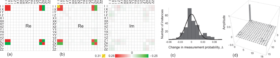
Figure 1: (color) Process matrix of the cnot gate epaps . (a) Ideal process matrix, in the basis defined by tensor products of Pauli operators (imaginary part is identically zero). (b) Maximum-likelihood experimental process matrix. (c) Histogram of the differences in probability between experimental data and the maximum-likelihood reconstruction for the 256 tomographic measurements. The Gaussian fit $\gamma\exp(-\Delta^{2}/\sigma^{2})$ has $\sigma=0.021$. (d) Real part of the experimentally determined process matrix, expressed in the cnot operator basis, where the 00 element represents the component of $U_{\rm CNOT}$ in the process. The elements’ imaginary parts are negligible, except for one coherence of magnitude 0.06. In this basis, an ideal cnot has a unit-valued 00 element; all other elements are zero. The abscissae are the abscissae of (a) and (b), multiplied by $\hat{U}_{\rm CNOT}.$

How well does the matrix $\tilde{\chi}$ describe the raw data? Clearly there will be some discrepancy, as the simple matrix inversion (i.e. without maximum-likelihood estimation) produces an unphysical process matrix. It is possible to obtain information about the confidence of the fit by examining the residuals (Fig. 1(c)), i.e. the differences $\Delta$ between each of the 256 measurement probabilities and the corresponding probabilities predicted from $\tilde{\chi}$. The width of this distribution, $\sigma(\Delta)=0.021$, gives an idea of the relative error in the process tomography. We further test the maximum-likelihood technique by comparing the predicted output state predicted by $\tilde{\chi}$) with the experimentally determined output state for all 16 inputs. The average fidelity and standard deviation between the predicted and measured density matrices are 0.95 and 0.03, respectively.

Ultimately, we want to characterize the process relative to some ideal: in this case, $\chi_{\rm\textsc{cnot}}$, which is the process matrix representing $\hat{U}_{\rm CNOT}$ White et al. (2003). We use the process fidelity Gilchrist et al. (2003), $F_{P}={\rm Tr}\left(\chi_{\rm\textsc{cnot}}\hskip 2.0pt\tilde{\chi}\right)$, and find $F_{P}=0.87$. We can obtain a graphical representation of $F_{P}$ by expressing the process matrix in the “cnot” basis (obtained by acting $\hat{U}_{\rm CNOT}$ on all the Pauli basis elements). In this case, $F_{P}$ is simply the height of the corner (00) element, as shown in Fig. 1(d). Currently, we are not able to put an error bar on $F_{P}$ when it is calculated from $\tilde{\chi}$. The only known technique for obtaining error estimates on the elements of the process matrix comes from performing many reconstructions of the process matrix with random noise added to the raw data in each case Mitchell et al. (2003). The incorporation of the extra constraints for trace-preservation slows down the numerical minimization to the point where it is impractical to consider repeating the fitting procedure for many simulated data sets.

The fact that the fidelity of the process is given by the height of one element of $\tilde{\chi}$ in the cnot basis suggests that $F_{P}$ might be obtained with far fewer experimental settings than for full QPT. In principle, only $d^{2}$ parameters are required to find $F_{P}$. For our (physically achievable) settings qpt (a), the process fidelity with the ideal cnot can be calculated directly from a 71-element subset of the tomographic data. Importantly, any such “direct” relationships Barbieri et al. (2003) also allow straightforward error estimates. Using this alternative technique, we find $F^{\prime}_{P}=0.93\pm 0.01$ qpt (c). The error bar is smaller than $F^{\prime}_{P}-F_{P}$, however, the error in $F_{P}$ is not presently known.

The average gate fidelity $\overline{F}$ Nielsen (2002) is defined as the state fidelity qpt (d) between the actual and ideal gate outputs, averaged over all input states. There is a simple relationship between the process fidelity and the average fidelity for any process Gilchrist et al. (2003), which we apply with our data: $\overline{F}^{\prime}=(d\hskip 1.0ptF_{P}^{\prime}+1)/(d+1)=0.95\pm 0.01.$ We believe that the sub-unit fidelity primarily arises from imperfect mode matching (spatial and spectral overlap of the optical beams). Mode mismatch results in imperfect nonclassical interference between control and target photons, and mixture of the individual qubit states as well. Mode mismatch is not a fundamental limitation for optical quantum gates, and guided mode implementations promise an elegant solution. Nonclassical interferences with $>99\%$ visibility have been observed with single photons and guided mode beamsplitters Pittman and Franson (2003).

Although the fidelity may seem like a simple method for comparing processes, it is not ideal, because it does not satisfy many of the requirements for a good measure. A full list of the desirable properties can be found elsewhere (e.g. Ref. Gilchrist et al. (2003)), but to some extent they can be summarized by the concept that an ideal measure must remain valid when used to characterize a gate as part of a larger quantum circuit, as well as in isolation. To this end, a more appropriate measure, $C_{P}=\sqrt{1-F^{\prime}_{P}}$ has been developed. Although monotonically related to the process fidelity, it has all the properties required. $C_{P}$ is a metric, so that two processes that are identical will have $C_{P}=0$; orthogonal processes have $C_{P}=1$. The operational interpretation of $C_{P}$ is that the average probability of error $\overline{P}_{E}$ for a quantum computer circuit used to compute some function obeys $\overline{P}_{E}\leq{C_{P}}^{2}$ Gilchrist et al. (2003). For our gate, $\overline{P}_{E}\leq 0.07\pm 0.01$.

We also introduce a simple relation to characterize how much mixture our gate introduces (for details, seeGilchrist et al. (2003)): $\overline{{\rm Tr}\left(\rho^{2}\right)}=(d\hskip 1.0pt{\rm Tr}(\tilde{\chi}^{2})+1)/(d+1)=0.83,$ where the quantity on the left hand side is the purity of gate output states, averaged over all pure inputs. This corresponds to an average normalized linear entropy White et al. (2001) of 0.22.

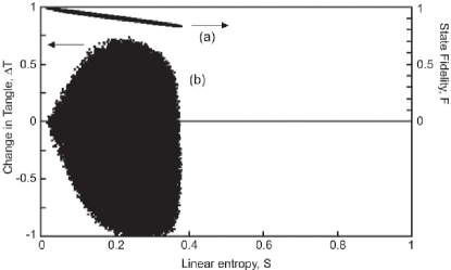
Figure 2: (a) State fidelity of our cnot gate outputs (with ideal cnot output states) calculated from $\tilde{\chi}$, plotted against the linear entropy added by the gate. A perfect experimental cnot process would have F=1, S=0 for all states. (b) Change in tangle between input and output, and linear entropy added, for our cnot gate outputs, calculated from $\tilde{\chi}$. An ideal cnot would have points with $\Delta T$ distributed between -1 and 1, and S=0.

An instructive method for examining the action of the gate, in terms of fidelity, entanglement (quantified by the tangle T White et al. (2001, 2001)) and entropy, is to make scatter plots of these quantities for output states of the gate (Fig. 2). We used $\sim$200000 pure, uniformly distributed (by the Háar measure) input states, and the $\tilde{\chi}$ matrix, to predict a distribution of output states of our experimental gate. From this data, we can observe the relationship between the mixture added, and both the entanglement generated by the gate and the gate output state fidelity. The gate has three separate spatial mode matching conditions O’Brien et al. (2003), and the contribution of each of these to the overall mixture is state dependent, leading to the distribution of entropies. There is a clear correlation between the fidelity and the amount of mixture added, and the minimum output state fidelity is 0.83. The shape of the upper lobe ($\Delta T>0$) of the $\Delta T\hskip 2.0pt{\rm vs.}\hskip 2.0ptS$ plot (Fig. 2(b)) is readily understood by the state-dependent mode matching considerations. States that have the largest change in tangle correspond to cases when the gate requires all three mode matching conditions to be simultaneously satisfied, and since each is not perfectly satisfied, this introduces some mixture. There exist partially entangled input states for which $\Delta T\approx 0$ and all three mode matching conditions apply, and these also have higher entropy. When only one mode matching condition applies, the gate cannot perform an entangling operation, but only a little mixture is added. The extension of the lower lobe ($\Delta T<0$) to $\Delta T=-1$ (asymmetric with the upper lobe) can be explained by the fact that when the gate acts to disentangle the input, the addition of mixture also reduces the tangle. We find that the maximum increase in tangle of the gate (the entangling capability Poyatos et al. (1997)) is $\Delta T_{\rm max}=0.73$.

In summary, we have demonstrated the full characterization of a two-qubit entangling quantum process – a controlled-NOT gate – by applying physical quantum process tomography. With the process matrix, we can predict, with approximately $95\%$ fidelity, the action of the gate on an arbitrary two-qubit input state. We determine: an average gate fidelity of 0.90 using the process matrix, and $0.95\pm 0.01$ using a set of 71 input and measurement settings; an average error probability bounded above by 0.07 $\pm$ 0.01; and a maximum increase in tangle of 0.73. The main failure mechanism of the gate can be observed from the process matrix in the Pauli basis, and the scatter plots – some of the operator population is incoherently redistributed so that the gate performs the identity operation with higher probability than for the ideal cnot, a mechanism that we assign primarily to the imperfect mode matching of the interferometers.

We thank M.J. Bremner, J.S. Lundeen, M.W. Mitchell, M.A. Nielsen, and S. Schneider for helpful discussions. This work was supported in part by the Australian Research Council, and the NSA and ARDA under ARO Contract No. DAAD-19-01-1-0651. AG acknowledges support from the NZ FRST. DFVJ acknowledges support from the MURI Center for Photonic Quantum Information Systems (ARO/ARDA program DAAD19-03-1-0199).

References

- Nielsen and Chuang (2000) M.A. Nielsen and I.L. Chuang, Quantum Computation and Quantum Information (Cambridge University Press, Cambridge, 2000).
- Gisin et al. (2002) N. Gisin, et al., Rev. Mod. Phys. 74, 145 (2002).
- Dowling and Milburn (2003) J.P. Dowling and G.J. Milburn, Philos. Trans. R. Soc. London, Ser. A 361, 1655 (2003).
- Knill et al. (2001) E. Knill, R. Laflamme, and G.J. Milburn, Nature 409, 46 (2001).
- (5) M.A. Nielsen, Phys. Rev. Lett. 93, 040503 (2004).
- Pittman et al. (2001) T.B. Pittman, B.C. Jacobs, and J.D. Franson, Phys. Rev. A 64, 062311 (2001).
- Koashi et al. (2001) M. Koashi, T. Yamamoto, and N. Imoto, Phys. Rev. A 63, 030301 (2001).
- Pryde et al. (2003) G.J. Pryde, et al., Phys. Rev. Lett. 92, 190402 (2003).
- Kok et al. (2002) P. Kok, H. Lee, and J.P. Dowling, Phys. Rev. A 66, 063814 (2002).
- Pryde and White (2003) G.J. Pryde and A.G. White, Phys. Rev. A 68, 052315 (2003).
- Chuang and Nielsen (1997) I.L. Chuang and M.A. Nielsen, J. Mod. Opt. 44, 2455 (1997).
- Poyatos et al. (1997) J.F. Poyatos, J.I. Cirac, and P. Zoller, Phys. Rev. Lett. 78, 390 (1997).
- Nielsen et al. (1998) M.A. Nielsen, E. Knill, and R. Laflamme, Nature 396, 52 (1998).
- Childs et al. (2001) A.M. Childs, I.L. Chuang, and D.W. Leung, Phys. Rev. A 64, 012314 (2001).
- Altepeter et al. (2003) J.B. Altepeter, et al., Phys. Rev. Lett. 90, 193601 (2003).
- De Martini et al. (2003) F. De Martini, et al., Phys. Rev. A 67, 062307 (2003).
- Nambu et al. (2002) Y. Nambu, et al., Proc. SPIE 4917, 13 (2002).
- Mitchell et al. (2003) M.W. Mitchell, et al., Phys. Rev. Lett. 91, 120402 (2003).
- O’Brien et al. (2003) J.L. O’Brien, et al., Nature 426, 264 (2003).
- James et al. (2001) D. F. V. James, et al., Phys. Rev. A 64, 052312 (2001).
- qpt (a) There are an infinite number of such bases, so there is substantial flexibility in choosing tomographic input and measurement settings. We encode qubits in polarization, with and . Then and . Our QPT input states are taken from {HH, VH, DV, LH, LV, VV, HV, HA, HL, LL, LA, DA, DR, VA, VL, DH} and measurements from {HH, HV, VH, VV, HD, HL, VL, VD, DD, RL, RD, DR, DV, RV, DH, RH}.
- D’Ariano (2001) G.M. D’Ariano and P. Lo Presti, Phys. Rev. Lett. 86, 4195 (2001); G.M. D’Ariano and P. Lo Presti, Phys. Rev. Lett. 91, 047902 (2003)
- qpt (b) The postselective nature of our experiments precludes maps that are not trace-preserving (e.g., where one or more photons are lost). For non-trace-preserving processes,
- qpt (c) We use the NMinimize routine in
- Jezek et al. (2003) M. Ježek, J. Fiurášek, and Z. Hradil, Phys. Rev. A 68, 012305 (2003).
- Jamiolkowski (1972) A. Jamiolkowski, Rep. Math. Phys. 3, 275 (1972).
- Gilchrist et al. (2003) A. Gilchrist, N.K. Langford, and M.A. Nielsen, quant-ph/0408063 (2004).
- White et al. (2003) A.G. White, et al., quant-ph/0308115 (2003).
- Barbieri et al. (2003) M. Barbieri, et al., Phys. Rev. Lett. 91, 227901 (2003).
- qpt (c) Errors calculated from Poissonian counting statistics.
- Nielsen (2002) M.A. Nielsen, quant-ph/0205035 (2002).
- qpt (d) For density matrices and , .
- Pittman and Franson (2003) T.B. Pittman and J.D. Franson, Phys. Rev. Lett. 90, 240401 (2003).
- White et al. (2001) A.G. White, et al., Phys. Rev. A 65, 012301 (2001).
- White et al. (2001) W.K. Wootters, Phys. Rev. Lett. 80, 2245 (1998)
- (36) See EPAPS Document No. E-PRLTAO-93-016432 for numerical values of , and our cnot truth table. A direct link to this document may be found in the online article’s HTML reference section. The document may also be reached via the EPAPS homepage (http://www.aip.org/pubservs/epaps.html) or from ftp.aip.org in the directory /epaps/. See the EPAPS homepage for more information.