Storing Images in Entangled Quantum Systems

Abstract

We introduce a new method of storing visual information in Quantum Mechanical systems which has certain advantages over more restricted classical memory devices. To do this we employ uniquely Quantum Mechanical properties such as Entanglement in order to store information concerning the position and shape of simple objects.

I Introduction

The storage, processing and retrieval of visual information are first order tasks for researchers in the discipline of Image Processing and related areas such as Pattern Recognition and Artificial Intelligence. However, due to the restricted architecture of classical computers and the often overwhelming computational complexity of state-of-the-art algorithms, it is necessary to find better ways to store, process and retrieve visual information.

In a classical memory device, memory cells are, in terms of hardware, independent of one another, that is, each storage location can be ascribed a reality that is independent of all other locations in the memory. Furthermore, such independence is actually inherited by any kind of information stored in such memory cells. The only way to correlate values stored in a classical computer memory is by means of software.

Thus, storing an image in a classical Von Neumann computer involves a memory which essentially consists of a large set of independent bits, each of which represents some property of the associated image, for example light intensity. Recovery of information concerning the image involves reading binary data stored in the computer memory, that is, an image is recovered by performing independent measurements of a physical property, that of electric potential difference, on each cell of the memory device. However, correlations between different points in an image are very important in order to properly understand and describe it. Typically, any one part of an image bears an important relation to other parts. Since the bits that are used to store such images in a classical Von Neumann computer are essentially independent of one another, much relevant information pertaining to the image may be lost upon classical data storage. Alternative methods for data storage and processing have been proposed in the past in order to overcome such loss of information. Among them, associative memories stand in first place kohonen . However, associative memories is an inefficient proposal as the number of patterns that can be stored in a $n$-bit associative memory is $O(n)$. A recent development by Trugenberger trugenberger shows that it is possible to use a multi-particle quantum system to implement an efficient quantum associative memory.

Methods for data storage, processing and retrieval form a broad and active field of research in Quantum Information Processing. In the next section we review some of the more general principles of Quantum Information before specializing in later sections to the subject of image storage and retrieval.

II Quantum vs. Classical Computation

We shall devote this section to an analysis of some fundamental elements of Quantum Mechanics used in Quantum Computation (QC) and Quantum Information Processing (QIP).

We start by exploring the differences between the basic information storage components of classical and quantum computers, namely bits and qubits. This topic is important due to the non-trivial physical structure of a qubit and its corresponding mathematical representation. We also study in this section how sets of qubits interact and combine, as well reviewing the mathematical representation of a quantum system composed of $n$ qubits.

Following this we briefly explain the theory of measurement in Quantum Mechanics. Measuring in quantum mechanics is far from being either intuitive or trivial. In fact, measurement is one of the most striking features of quantum theory and the concept of measurement strategy plays a most important role in information extraction in QC and QIP.

Finally, we look at a unique property of quantum systems that has no equivalent in the world of classical physics: quantum Entanglement. Entanglement is a unique type of correlation shared between components of a quantum system. Entangled quantum systems are often best used collectively, that is, an optimal use of entangled quantum systems for information storage and retrieval must manipulate and measure those systems as a whole, rather than on an individual basis.

Entanglement has emerged as a key concept in QC and QIP as it is used as a physical resource to build quantum algorithms shor ; grover as well as to develop schemes for quantum teleportation bennett .

II.1 Classical bits vs. Qubits

Mathematical representations of a classical bit and a single qubit

In recent years, progress in the field of Quantum Computation and Quantum Information has taught computer scientists that nature can be harnessed far more efficiently for computation by exploiting quantum-mechanical properties of systems. In 1985 Deutsch developed a theoretical machine, the Universal Quantum Turing Machine, which is a generalization of the Universal Turing Machine deutsch . Such a Quantum Computer, which performs computations according to the rules of Quantum Mechanics, is capable of performing certain tasks more efficiently than its classical counterpart. Two celebrated examples of such tasks are the factorization of large numbers in Shor’s algorithm shor and the search for a data item in an unordered database in Grover’s algorithm grover .

In Classical Computation, information is stored and manipulated in the form of bits. The mathematical structure of a classical bit is rather simple. It suffices to define two ‘logical’ values, traditionally labelled as $\{0,1\}$, and to relate these values to two different outcomes of a classical measurement. So a classical bit ‘lives’ in a scalar space.

In Quantum Computation, information is stored, manipulated and measured in the form of qubits. A qubit is a physical entity described by the laws of Quantum Mechanics. Simple examples of qubits include two orthogonal polarizations of a photon (e.g. horizontal and vertical), the alignment of a (spin-1/2) nuclear spin in a magnetic field or two states of an electron orbiting an atom. A qubit may be mathematically represented as a vector $|\Psi\rangle$ in a two-dimensional complex vector space which has an associated inner product, so $|\Psi\rangle\in{\cal H}^{2}$. For the sake of this discussion, we refer to such a vector space as a two-dimensional Hilbert space ${\cal H}^{2}$.

The notation $|\rangle$, a ket, is part of the Dirac notation, a standard and very convenient typography in Quantum Mechanics which actually is far more than mere notation.

A qubit $|\Psi\rangle$ may be written in general form as

$$|\Psi\rangle=\alpha|p\rangle+\beta|q\rangle$$ (1)

where the complex coefficients $\alpha$ and $\beta$ satisfy the normalization condition $|\alpha|^{2}+|\beta|^{2}=1$ and $\{|p\rangle,|q\rangle\}$ is an arbitrary basis spanning ${\cal H}^{2}$. The choice of $\{|p\rangle,|q\rangle\}$ is often $\{|0\rangle,|1\rangle\}$. These are the computational basis states and form an orthonormal basis for the qubit vector space. So in general $|\Psi\rangle$ is a coherent superposition of the basis states $|p\rangle$ and $|q\rangle$ and can be prepared in an infinite number of ways simply by varying the values of the complex coefficients $\alpha$ and $\beta$ subject to the normalization constraint. In contrast, classical computers measure bit values using only one basis, $\{0,1\}$, and the only two possible states are those that correspond to the measurement outcomes 0 or 1.

A qubit can also be represented by a density operator (often the density matrix is used in the literature). Both representations are equivalent, thus using one representation or the other depends on the properties of the system to be studied. The density operator of a qubit is usually denoted as $\hat{\varrho}$.

For example, it is a good idea to use a vector representation in problems where we know with certainty the initial state of the qubit. An example of this statement is to have a qubit prepared in the state $|\Psi\rangle=\frac{|0\rangle+|1\rangle}{\sqrt{2}}$, that is, an equally weighted superposition of the canonical basis $\{|0\rangle,|1\rangle\}$.

However, let us consider a different scenario in which a qubit $|\Psi\rangle$ is initially prepared in one of the following quantum states: $\{|\psi\rangle_{1},|\psi\rangle_{2},|\psi\rangle_{3},\ldots,|\psi\rangle_{n}\}$ where each of the states is selected with probability $\frac{1}{n}$. We do not know what state was chosen to prepare $|\Psi\rangle$, but we do know that only preparations $|\psi\rangle_{i}$, $i\in\{1,2,\ldots,n\}$ are allowed. In this case, a convenient representation for $|\Psi\rangle$ is the associated density operator

$$\hat{\varrho}_{\Psi}={1\over n}\sum\limits_{k=1}^{n}|\psi\rangle_{k}{}_{k}\langle\psi|$$ (2)

The symbol $\langle|$ denotes a bra, another symbol from Dirac notation. $\langle\psi|$ is alternatively written as $|\psi\rangle^{\dagger}$, the complex conjugate transpose of $|\psi\rangle$. As an example, let us set $|\psi\rangle=\begin{pmatrix}0\\ 1\end{pmatrix}$ for the computational basis $\{|0\rangle,|1\rangle\}$. Then, $\langle\psi|=\begin{pmatrix}0&1\end{pmatrix}$. Taking the inner product yields $\langle\psi|\psi\rangle=\begin{pmatrix}0&1\end{pmatrix}\begin{pmatrix}0\\ 1\end{pmatrix}=1$ i.e. the inner product of $|\psi\rangle$ with itself is unity.

Mathematical representation of an array of qubits

A composite qubit system $|\Phi\rangle$, often also called a qubit array, is a quantum system made up of several qubits, where each qubit is associated with a two-dimensional Hilbert space ${\cal H}^{2}$. The postulates of Quantum Mechanics establish that the vector space where a composite qubit system lives is the tensor product of the vector spaces of the component physical systems. Thus, if component qubits are $|\psi\rangle_{1},|\psi\rangle_{2},\ldots,|\psi\rangle_{n}$ (where each qubit resides in a two-dimensional Hilbert space ${\cal H}^{2}$) then $|\Phi\rangle$ lives in a Hilbert space ${\cal H}^{2^{n}}={\cal H}^{2}\otimes{\cal H}^{2}\otimes\ldots\otimes{\cal H}^{2}$.

A simple classical data storage device can be considered as an array made up of $n$ classical bits and capable of storing one of $2^{n}$ different classical bit strings. A simple quantum memory device is a qubit array. Such a data storage device consists of $n$ qubits. Each is prepared in some quantum state determined by the desired information to be stored in that particular qubit. Thus, in principle, both classical and quantum arrays can store up to $2^{n}$ different values. However, in stark contrast to classical data storage, an array of $n$ qubits is capable of storing in a coherent superposition $2^{n}$ different bit strings simultaneously trugenberger .

Excellent introductions to vector and density matrix representations for single and multiple qubits can be found in rieffel ; nielsen .

II.2 Quantum Measurement

Measurement according to the rules of Quantum Mechanics is a non-trivial and highly counter-intuitive process. Firstly, it must be said that the measurement results taken from a quantum system are inherently of a probabilistic nature. In other words, regardless of the carefulness in the preparation of a measurement procedure, the possible outcomes of such measurement will be distributed according to a certain probability distribution.

Secondly, once a measurement has been performed, a quantum system in unavoidably altered due to the interaction with the measurement apparatus. Thus, it makes sense to talk about pre-measurement and post-measurement quantum states for an arbitrary quantum system.

Thirdly, in order to perform a measurement it is needed to define a set of measurement operators. This set of operators must fulfill a number of rules that allows one to compute the actual probability distribution as well as post-measurement quantum states.

In order to clarify these points, let us work out a simple example. Assume we have a polarized photon with associated polarization orientations ‘horizontal’ and ‘vertical’. The horizontal polarization direction is denoted by $|0\rangle$ and the vertical polarization direction is denoted by $|1\rangle$.

Thus, an arbitrary initial state for our photon can be described by the state by $|\Psi\rangle=\alpha|0\rangle+\beta|1\rangle$, where $\alpha$ and $\beta$ are complex numbers constrained by the normalization condition $|\alpha|^{2}+|\beta|^{2}=1$ and $\{|0\rangle,|1\rangle\}$ is the computational basis spanning ${\cal H}^{2}$.

Now, let us construct two measurement operators $\hat{M}_{0}=|0\rangle\langle 0|$ and $\hat{M}_{1}=|1\rangle\langle 1|$ and two measurement outcomes $a_{0},a_{1}$. Then, the full observable used for measurement in this experiment is $\hat{M}=a_{0}|0\rangle\langle 0|+a_{1}|1\rangle\langle 1|$.

According to the rules of Quantum Mechanics, the probabilities of obtaining outcome $a_{0}$ or outcome $a_{1}$ are given by $p(a_{0})=|\alpha|^{2}$ and $p(a_{1})=|\beta|^{2}$. Corresponding post-measurement quantum states are as follows: if outcome $=a_{0}$ then $|\Psi_{pm}\rangle=|0\rangle$; if outcome $=a_{1}$ then $|\Psi_{pm}\rangle=|1\rangle$.

It is possible to construct a full quantum measurement theory for both vector and density matrix representations of quantum systems (for a review, see nielsen ). Measurement theory and its implications in QC and QIP are open and fruitful fields of research.

II.3 Quantum Entanglement

Quantum Entanglement is a key concept in QC and QIP. We shall review the experiments that sparked an investigation into quantum entanglement as well as the mathematical structure of some entangled states widely used in QC and QIP.

The concept of correlation is deeply rooted in every branch of science. A typical and simple example is the following experiment: let us suppose we have two balls, one white and one black, as well as two boxes. If we randomly put a ball in each box and then close both boxes, we need to perform only one experiment, that is, to open one box, in order to know which of the balls is in each box. In other words, by means of one measurement, opening one box and seeing which ball was stored in it, we obtain two pieces of information, namely the colour of the ball stored in both boxes.

The former experiment is an example of classical correlation. Quantum entanglement is also a kind of correlation, but one that is detected only in quantum phenomena.

Quantum systems can be tested for inherent entanglement using various measurement procedures. During the development of Quantum Mechanics as a physical theory, it was discovered that it is either an incomplete theory of nature, or that it is nonlocal, meaning that something which happens spontaneously at one place instantaneously influences what is true at another place (for historical discussion see e.g. EPR ). In order to prove that Quantum Mechanics is not an incomplete theory, John Bell developed a series of inequalities to test the validity of Quantum Mechanics (for a more detailed discussion see e.g. bell ). Violation of the bipartite Bell inequalities implies that some quantum-mechanical predictions cannot be reproduced by a local hiddenvariable model.

Before elaborating more on Bell inequalities, let us review the mathematical appearance of entangled systems for simple cases.

For example, consider the following 2-particle state:

$$|\Psi_{-}\rangle=\frac{|01\rangle-|10\rangle}{\sqrt{2}}$$ (3)

(This is the famous EPR/singlet state which appears in many discussions of non-locality). Clearly, $|\Psi_{-}\rangle$ lives in a four-dimensional Hilbert space. It can be seen, after some calculations, that it is impossible to find quantum states $|a\rangle,|b\rangle\in{\cal H}^{2}$ such that $|a\rangle\otimes|b\rangle=|\Psi\rangle$, that is, $|\Psi\rangle$ is not a product state of $|a\rangle$ and $|b\rangle$. This is indeed a criterion to determine whether a quantum state is entangled or not, whether it is possible to express such a composite quantum state as a simple tensor product of quantum subsystems.

Another example is the tripartite entangled GHZ state

$$|\text{GHZ}\rangle=\frac{|000\rangle+|111\rangle}{\sqrt{2}}$$ (4)

Again, it is not possible to find three quantum states $|a\rangle,|b\rangle,|c\rangle\in{\cal H}^{2}$ such that $|a\rangle\otimes|b\rangle\otimes|c\rangle=|\text{GHZ}\rangle$.

It must be said that entanglement definition and quantification is an open research area. Currently it is known how to identify and quantify entanglement for two particles. For three or more particles the situation is far less straightforward and remains an active area of research.

Let us now turn to some basic definitions and extensions of the previous theory in the density matrix formalism. Consider a bipartite system with Hilbert space ${\cal H}={\cal H}_{1}\otimes{\cal H}_{2}$. Suppose that two qubits reside in the joint state $|\Psi\rangle_{12}$. This state is said to be separable if it is possible to write $|\Psi\rangle_{12}=|\Psi\rangle_{1}\otimes|\Psi\rangle_{2}$. Such a bipartite state may instead be written in terms of its density matrix $\hat{\varrho}$ ($\hat{\varrho}=|\Psi\rangle\langle\Psi|$ for a pure state $|\Psi\rangle$), in which case any separable state may be written as a convex sum of direct-product states

$$\hat{\varrho}^{(12)}=\sum_{i}p_{i}\hat{\varrho}^{(1)}_{i}\otimes\hat{\varrho}^{(2)}_{i}$$ (5)

where the $p_{i}$ represent probabilities satisfying the condition $\sum_{i}p_{i}=1$. An entangled state is a state which cannot be written in the form of Eq. (5) above. In this case, it is impossible to ascribe an independent reality to either of the two subsystems separately. Instead, they share only a collective reality.

The basic concepts of bipartite entanglement may be extended to the multipartite case. For example, a tripartite state is unentangled if it is possible to write the associated density matrix in the form

$$\hat{\varrho}^{(123)}=\sum_{ijk}p_{ijk}\hat{\varrho}^{(1)}_{i}\otimes\hat{\varrho}^{(2)}_{j}\otimes\hat{\varrho}^{(3)}_{k}$$ (6)

where $\hat{\varrho}^{(1)}_{i},\hat{\varrho}^{(2)}_{j},\hat{\varrho}^{(3)}_{k}$ represent single-particle density matrices. A partially-entangled tripartite state may be written in the form

$$\hat{\varrho}^{(123)}=p_{r}\hat{\varrho}^{(12)}\otimes\hat{\varrho}^{(3)}+p_{s}\hat{\varrho}^{(13)}\otimes\hat{\varrho}^{(2)}+p_{t}\hat{\varrho}^{(23)}\otimes\hat{\varrho}^{(1)}$$ (7)

where the $\hat{\varrho}^{(ij)}$ represent entangled states of two of the subsystems involved. Any state $\hat{\varrho}^{(123)}$ that obeys $\hat{\varrho}^{(123)}\neq\sum_{i}p_{i}\hat{\varrho}_{i}$, where all the $\hat{\varrho}_{i}$ are separable into products of states of less than three parties, is fully entangled.

For an $N$-qubit system, following state can be defined and will prove useful in what follows:

$$|\Psi_{N}\rangle=\frac{|0\rangle^{\otimes N}+|1\rangle^{\otimes N}}{\sqrt{2}}$$ (8)

This state is often referred to as the $N$-particle GHZ state (see e.g.GHZ ). States of this form can be produced to a good approximation in quantum optical systems. Experimental realizations are presented in rausch ; sackett ; pan , where it is discussed that states with $N$ up to 4 have already been produced.

In certain cases Bell inequalities may also be used to detect the presence of entanglement. Bell-type inequalities for $N$-particle systems have been derived under the assumption of total and partial separability and provide us with a way of deciding whether a set of $N$ particles resides in a maximally entangled state (see e.g. the Seevinck-Svetlichny inequalities svetlichny2 ; gisinbell ). Such inequalities also provide, upon violation, experimentally accessible conditions for full $N$-particle entanglement and will prove very useful in what follows.

III New method for storing images

In the discussion that follows, we focus our attention on simple binary images (those images having only two brightness levels, black and white). Such images can be obtained quite simply by thresholding any gray-level image. Whilst restricted in application, such images are of interest because they are relatively straightforward to process and therefore provide a useful starting point for introducing Entanglement in the context of image processing.

III.1 Storage of information

We aim to store information concerning the structure and content of a simple image in a quantum system. Consider an array of $n$ qubits which we propose to use as our memory storage. Each qubit in the array may be associated with two parameters, $x$ and $y$, which together represent grid points of some simple 2D image. Such an array can therefore be used to store visual information. Prior to inputting information into the array, we suppose that each qubit is initialized to state $|0\rangle$. The initial state of the memory is therefore given by the following expression

$$|\Psi_{\text{initial}}\rangle=\bigotimes^{n}_{i=1}|0\rangle_{i(x,y)}$$ (9)

We wish to store information about the position and shape of certain simple objects which are represented on our grid as collections of points. Extending the classical binary image formalism to qubits, we associate a white point on the grid with qubit state $|0\rangle$, whilst black corresponds to state $|1\rangle$. However certain extensions of the classical approach are necessary to fully exploit the unique properties of Entanglement. A simple example will suffice to explain the principles of such a quantum storage device.

Suppose that we wish to store the shape of a triangle in our qubit array. In this case, we might choose to represent each vertex of the triangle on the grid by setting the corresponding qubit to $|1\rangle$. Such a procedure is depicted in Fig. (1).

The appropriate vertex positions may then be retrieved by applying Grover’s quantum search algorithm to the array. We would expect that searching an $n$-qubit array for a $|1\rangle$ using a classical algorithm would take approximately $O(n)$ steps. However, Grover’s quantum search algorithm can achieve such a task in approximately $O(\sqrt{n})$ steps due to its use of Quantum Mechanics. For three vertices stored in the array, application of Grover’s search algorithm will require approximately $\sqrt{n/3}$ steps to recover the information specifying the locations of the vertices of the triangle. The image of the triangle is then very simply reconstructed from this information.

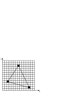
Figure 1: Simple storage procedure for a single triangle in a qubit array. In the classical approach, vertex positions correspond to qubit state $|1\rangle$ and the triangle image can be straightforwardly reconstructed. However, the use of Entanglement between vertex locations (dotted lines) provides a more fruitful approach.

However, suppose that we instead wish to store two triangles in the array. We could proceed as before with an essentially classical approach, preparing the qubits corresponding to triangle vertices in state $|1\rangle$ whilst all others remain in state $|0\rangle$. However, retrieval of information on vertex position by applying Grover’s search algorithm will not reveal anything about which vertices belong to which triangles. We need to store additional information in the array concerning which vertex points belong to which triangle. In this case, Entanglement may be employed to establish nonlocal correlations between the qubits storing the vertex locations of the same triangle. Consider again the maximally-entangled tripartite state

$$|\text{GHZ}\rangle=\frac{|000\rangle+|111\rangle}{\sqrt{2}}$$ (10)

Suppose that our qubit array stores a triangle by preparing the associated vertex qubits $\{p,q,r\}$ in a GHZ state. In this case, the memory state of the qubit array is

$$|\Psi_{\text{1 triangle}}\rangle=\otimes^{n}_{i=1,i\neq p,q,r}|0\rangle_{i}\otimes\frac{|000\rangle_{pqr}+|111\rangle_{pqr}}{\sqrt{2}}$$ (11)

Input of a second triangle with corresponding vertex qubits $\{s,t,u\}$ into the array yields memory state

$$|\Psi_{\text{2 triangles}}\rangle=\otimes^{n}_{i=1,i\neq p,q,r,s,t,u}|0\rangle_{i}\otimes|\text{GHZ}\rangle_{pqr}\otimes|\text{GHZ}\rangle_{stu}$$ (12)

Retrieval of the information regarding which particles reside in such maximally entangled states is therefore sufficient to locate the positions of the triangle vertices and also learn to which triangle they belong, as depicted in Fig. (2).

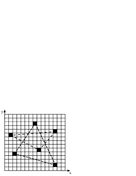
Figure 2: When two distinct shapes are stored in the array, entanglement (represented by dashed lines) between vertices belonging to the same shape is used to distinguish them from the other.

III.2 Retrieval

Once information about an image has been stored in the qubit array it is desirable to retrieve this information in order to reliably reconstruct the image. Information retrieval is achieved by way of performing measurements on the array.

Suppose that we store a triangle in the array in the form of the state $|\text{GHZ}\rangle_{pqr}$. Information pertaining to relations between one memory location for the image and another could be retrieved from the array by implementing the measurement projection operator

$$\hat{M}_{pqr}=|00...0\rangle|\text{GHZ}\rangle_{pqr}{}_{pqr}\langle\text{GHZ}|\langle 00...0|$$ (13)

where $|00...0\rangle$ acts on all qubits not belonging to the GHZ state. However, since any GHZ state consists of a coherent superposition of $|000\rangle$ and $|111\rangle$, the qubit array has the form of a coherent superposition $|\Psi_{\text{1 triangle}}\rangle=(1/\sqrt{2})(\otimes^{n}_{i=1}|0\rangle+\otimes^{n}_{i\neq p,q,r}|0\rangle\otimes|111\rangle_{pqr})=(1/\sqrt{2})(|\Psi_{\text{initial}}\rangle+\bigotimes^{n}_{i\neq p,q,r}|0\rangle_{i}\otimes|111\rangle_{pqr})$. In fact, any memory state of the qubit array will consist of a coherent superposition of $|\Psi_{\text{initial}}\rangle$ and other memory states. Therefore memory states associated with different images are nonorthogonal and cannot be distinguished unambiguously. This means that using projection operators will only give probabilistic results for vertex location and the image cannot be reliably reconstructed.

Instead, a measurement probing the entanglement shared between the vertex qubits is employed in order to determine their location. We illustrate this once again with our simple triangle example.

To search for triangles, a set of three qubits in the array is chosen for measurement. This tripartite state is then tested for violation of the Seevinck-Svetlichny inequalities for tripartite states. Violation implies the presence of full three-particle entanglement. Non-violation therefore implies that the three qubits selected do not form vertices of the same triangle. From this information it is straightforward to deduce the location of the triangle vertices. Now suppose that the three qubits selected consist of two qubits residing in the same GHZ state and a third that does not. Then the state to be tested is of the form presented in Eq. (7) and will not violate the appropriate inequalities for full tripartite entanglement. For our simple example of two triangles, determinations of the locations of all six vertices requires at worst ${}^{n}C_{3}.{}^{n-3}C_{3}$ different identically-prepared arrays to be tested for two instances of tripartite entanglement amongst different qubits.

Indeed, suppose that a shape in an image has $N$ vertices. In this case, an $N$-particle GHZ state is used to store such information. $N$-particle Bell-type inequalities that provide experimentally-accessible sufficient conditions for full $N$-particle entanglement have been derived (see references in Section 2) and therefore in principle our qubit array may be tested according to such inequalities to reveal vertex locations of more complex polygons.

Evidently the construction of a measurement procedure on the qubit array requires some a priori knowledge of the number and type of shapes stored in such an array. This information may be stored in a subset of the array qubits. Such a subset is addressed first in order to determine the appropriate number of qubits to pick from the array and test for shared entanglement, although this is not totally necessary.

III.3 Use of entanglement for scale-invariant shape recognition

We briefly note here that Entanglement may also be used to store and subsequently recognize various shapes in an image irrespective of their scale. It seems reasonable to suppose that a simple shape is recognized primarily by the number of vertices it has. Then storage of such a shape of any size in a qubit array where entanglement is shared between qubits corresponding to vertices of the same shape allows it to be recognized irrespective of its size. For example, the presence of a 4-particle GHZ state in a qubit array indicates that the stored image contains a shape with 4 sides. This information is of course unrelated to the scale of the shape (see Fig. (3). Of course, though, it is possible to locate the vertex qubits on the 2D grid and deduce the size of the object quite straightforwardly.

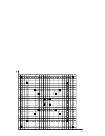
Figure 3: Simple illustration of scale-invariant shape recognition using entanglement in a 2D qubit array.

Storage of simple shapes using Entanglement also allows images that are stored in different memory arrays to be compared by measurement for similar or identical components simply by employing the procedures presented in Section IIIB.

IV Conclusions and Future Work

We have developed a novel method for storage and retrieval of simple binary images in Entangled quantum systems. Our work so far has concerned only binary images containing simple polygons. We hope to extend and generalize our work to gray-level images of increased structural complexity and present this work in a later paper.

References

- (1) T. Kohonen, Self Organization and Associative Memory. Springer Series in Information Sciences. Springer-Verlag, 1989.
- (2) Carlo Trugenberger, “Probabilistic Quantum Memories”, Phys. Rev. Lett. 87 p. 067901 (2001)
- (3) P. Shor, in Proceedings of the 35th Annual Symposium on the Foundations of Computer Science, Santa Fe, 1994, pp.124-134
- (4) L.K. Grover,“A fast quantum-mechanical algorithm for database search”, in Proceedings of the 28th annual ACM Symposium on Theory of Computing, Philadelphia, PA, May 1996, pp.212-219
- (5) C.H. Bennett, G. Brassard, C. Crepeau, R. Jozsa, A. Peres, and W. Wootters, “Teleporting an Unknown Quantum State via Dual Classical and EPR Channels”, Phys. Rev. Lett. 70 pp 1895 (1993)
- (6) David Deutsch, “Quantum Theory, the Church-Turing Principle and the Universal Quantum Computer”, in Proceedings of the Royal Society of London. Series A, Mathematical and Physical Sciences, Volume 400, Issue 1818, pages 97–117, July 8, 1985.
- (7) E. Rieffel and W. Polak, “An Introduction to Quantum Computing for Non-Physicists”, ACM Computing Surveys, Vol. 32(3), pp. 300–335, Sept. 2000
- (8) M.A. Nielsen and I.L. Chuang. “Quantum Computation and Quantum Information”, Cambridge University Press, Cambridge, UK, 2000.
- (9) A. Einstein, B. Podolsky and N. Rosen, Phys. Rev. Lett. 47, pp 777-780 (1935)
- (10) John S. Bell, “Speakable and Unspeakable in Quantum Mechanics”, Cambridge University Press, 1989.
- (11) M. Seevinck and G. Svetlichny, quant-ph/0201046
- (12) D. Collins, N. Gisin, S. Popescu, D. Roberts and V. Scarani, Phys. Rev. Lett. 88 170405 (2002)
- (13) D.M. Greenberger, M.A. Horne and A. Zeilinger in “Bell’s Theorem, Quantum Theory and Conceptions of the Universe” ed. M. Kafatos (Dordrecht, Kluwer 1989), D.M. Greenberger, M.A. Horne, A. Shimony and A. Zeilinger, Am. J. Phys. 58, 1131 (1990)
- (14) A. Rauschenbeutel et al, Science 288, 2024 (2000)
- (15) C. A. Sackett et al, Nature 404, 256 (2000)
- (16) J.-W. Pan, M. Daniell, S. Gasparoni, G. Weihs and A. Zeilinger, Phys. Rev. Lett. 86, 4435 (2001)