Laser linewidth effects in quantum state discrimination by EIT

Abstract

We discuss the use of electromagnetically modified absorption to achieve selective excitation in atoms: that is, the laser excitation of one transition while avoiding simultaneously exciting another transition whose frequency is the same as or close to that of the first. The selectivity which can be achieved in the presence of electromagnetically induced transparency (EIT) is limited by the decoherence rate of the dark state. We present exact analytical expressions for this effect, and also physical models and approximate expressions which give useful insights into the phenomena. When the laser frequencies are near-resonant with the single-photon atomic transitions, EIT is essential for achieving discrimination. When the laser frequencies are far detuned, the ‘bright’ two-photon Raman resonance is important for achieving selective excitation, while the ‘dark’ resonance (EIT) need not be. The application to laser cooling of a trapped atom is also discussed.

Electromagnetically-induced transparency (EIT, also called dark resonance or coherent population trapping) and phenomena related to it have been widely studied (see for example arimondo1996 ; book:scully and references therein). These two-photon resonance phenomena can give rise to sharp spectral features, which can be used for various purposes, including for example magnetometry and laser cooling fleischhauer1994 ; fleischhauer1995 ; aspect1988 ; lindberg1986 ; morigi2000 ; gea1995 . Recently, it was shown that EIT could be used to allow the angular momentum state of an atom to be detected with high quantum efficiency even in the absence of a Zeeman effect (i.e. at zero applied magnetic field and/or zero magnetic dipole moment of the atom) mcdonnell2003a . This paper develops the theory relevant to the latter, and sheds light on related experimental techniques such as laser cooling.

The essential concept here is the use of a two-photon resonance to achieve selective excitation in atoms. We are concerned with two states, generally closely-spaced, which have allowed transitions separated in frequency by a small interval (or coincident in frequency). We denote these states by $\left|{S}\right>$ and $\left|{I}\right>$, for ‘suppressed’ and ‘interacting’ respectively. Let $P_{S}$, $P_{I}$ be an experimentally observed signal, such as collected fluorescence, obtained when the atom is prepared in $\left|{S}\right>$ or $\left|{I}\right>$, respectively. We wish to irradiate the atom in such a way as to achieve a detectable signal $P_{I}$ and maximise the ratio $r\equiv P_{I}/P_{S}$.

The states $\left|{S}\right>$ and $\left|{I}\right>$ could for example be magnetic substates of the same atomic energy level, or they could represent the same internal state, but different motional states of an atom, such as two vibrational states in a harmonic potential well. In the former case, a high value for $r$ permits the atomic spin state to be detected mcdonnell2003a ; in the latter, a high value for $r$ implies that efficient laser cooling is possible lindberg1986 ; morigi2000 ; marzoli1994 ; reiss2002 .

Suppose the signal is collected fluorescence. Excitation out of a state $\left|{S}\right>$ can sometimes be avoided by using light of appropriate polarization. For example, with circularly polarized light driving the transition $n{\rm s}\,^{2}{\rm S}_{1/2}$–$n{\rm p}\,^{2}{\rm P}_{1/2}$, one of the ${}^{2}{\rm S}_{1/2}$ magnetic sublevels does not couple to the radiation. This would allow $P_{S}\simeq 0$ (limited only by experimental precision). However, in such a case the population of $\left|{I}\right>$ is rapidly lost by optical pumping to $\left|{S}\right>$, and hence $P_{I}$ is also small. Our interest here is in achieving high values of $r$ without significant transfer of population between $\left|{I}\right>$ and $\left|{S}\right>$.

The basic idea of using EIT, and more generally electromagnetically modified absorption (EMA), is illustrated in figure 1. We consider two situations. In the case illustrated in figure 1a, both $\left|{S}\right>$ and $\left|{I}\right>$ are connected by strong (e.g. electric-dipole allowed) transitions to upper states, such that the two transition frequencies are close together or even identical, but $\left|{S}\right>$ is part of a three-level manifold D which can exhibit dark resonance, while $\left|{I}\right>$ is not. In the case illustrated in figure 1b, both $\left|{S}\right>$ and $\left|{I}\right>$ are each part of separate three-level manifolds (called D and B for ‘dark’ and ‘bright’ respectively); both manifolds are driven simultaneously by a single pair of laser beams.

Suppose the detected signal were the fluorescence from the atom. In either case (a) or (b), if the laser frequencies are chosen in such a way that the D manifold is at a dark resonance, but the B manifold is not, then in the limit of no decoherence of the dark state, the ratio $r\rightarrow\infty$. This is evident when the manifolds D and B are not connected, since then excitation from $\left|{S}\right>$ will stop once the atom spontaneously enters the dark state, while excitation from $\left|{I}\right>$ can continue indefinitely. It is also true when the upper state of manifold D can decay to $\left|{I}\right>$ (which is more usual in practice), as long as we ensure an atom prepared in $\left|{S}\right>$ remains dark as the laser beams are introduced. This can be done by introducing the ‘pump’ laser, Rabi frequency $\Omega_{2}$ in figure 1, first, and then switching on the ‘probe’ laser of Rabi frequency $\Omega_{1}$ adiabatically, i.e. on a time-scale slow compared to the light-shift caused by the pump laser.

In practice the available value of $r$ is therefore limited by the loss of coherence of the dark state. For brevity we refer to this loss of coherence as a laser linewidth effect, although it can also be caused by other mechanisms. It is modelled simply as a decay rate $\gamma$ of the off-diagonal density matrix element $\rho_{21}$ in the Optical Bloch Equations for the D manifold. Note that many studies of phenomena related to EIT do not need to take this decoherence rate into account, except as a refinement, but here it is central.

Figure 1: Atomic level schemes considered in the text. a: $\left|{I}\right>$ is part of a two-level manifold, $\left|{S}\right>$ is part of a three-level manifold. b: $\left|{I}\right>$ and $\left|{S}\right>$ are each part of separate three-level manifolds. In either case, the atom is illuminated by a single pair of laser beams which drive both manifolds; the single photon transition 1–3 in the D manifold is either degenerate with or close to the single-photon transition out of $\left|{I}\right>$ in the B manifold. $\Omega_{1}$, $\Omega_{2}$ are Rabi frequencies, $\Gamma_{1}$, $\Gamma_{2}$ spontaneous decay rates, $\gamma$ is the rate of decay of coherence between levels 2 and 1. Both types of energy level structure are common in groups of atomic levels with $J\neq 0$. Case (b) also occurs in the combination of internal and vibrational states of a trapped atom.

We wish to understand the selectivity $r$ which can be achieved, as a function of all the relevant parameters. In order to do this, we model the atom as if the two manifolds $B$ and $D$ were not connected. If the excited state of $D$ can in fact decay to $B$ then such a model remains a good approximation as long as the population of the excited state of $D$ is small. It will be seen that this is the case when $r\gg 1$. On the other hand, if the excited state of $B$ can decay to $D$ then the model does not apply. (In any case this situation would result in optical pumping from $\left|{I}\right>$ to $\left|{S}\right>$ and hence only a small signal $P_{I}$.)

We assume the experimental signals $P_{S}$ and $P_{I}$ are proportional to the steady-state population of the excited state in the relevant manifold. This ignores a possible contribution from the initial transient behaviour, for example during adiabatic switching on of the laser beams. The ignored contribution is negligible when the time-scale on which the measured signal is obtained is long compared with the transient.

Our approach is to write down the steady state solution to the optical Bloch equations (OBEs) for a three-level atom excited by two laser fields of finite linewidth, and then examine the behaviour of this solution. The full solution is a rather complicated function of many parameters. In previous work it has been obtained and then studied in a simplified form under various restrictions, such as low pump power or zero detuning. One of the aims of this paper is to provide analytical expressions which retain as great a range of validity as possible, while being sufficiently simple to give clear general insights into the physical behaviour. This is done by finding factorisations of parts of the formulae, and by making good choices of the parameters with which to express them. We also present physical pictures to give further insight into the behaviour.

The work was motivated by the idea that the phenomenon of dark resonance ought to make available especially high values of $r$. Our results show, however, that this is only partially true.

We consider two regimes in detail: first the resonant case $\Delta_{1}=\Delta_{2}=0$, and then the far-detuned case $\Delta_{1}\gg\Gamma$ where $\Delta_{1}=\omega_{L1}-\omega_{31}$, $\Delta_{2}=\omega_{L2}-\omega_{32}$ are the detunings of the lasers from their respective single-photon transitions, and $\Gamma$ is the width of the upper state.

The case of figure 1a is interesting because it permits a high degree of state discrimination even when the single-photon transitions from $\left|{S}\right>$ and $\left|{I}\right>$ have the same frequency. In this situation frequency discrimination of the bare single-photon transitions is ruled out completely, hence the EMA is crucial to achieving any discrimination. It was shown in ref mcdonnell2003a that this can be used to measure an atomic spin state at zero magnetic field or zero magnetic dipole moment. The choice $\Delta_{1}=\Delta_{2}$ is used to make the dark resonance of the $D$ system as dark as possible, while setting both detunings equal to zero causes the $B$ system to give the maximum single-photon scattering rate. The value of $r$ is derived in section III; it is found to be proportional to the intensity of the pump laser in the D system, divided by $\gamma$.

In the case of figure 1b, both manifolds D and B exhibit the phenomena of dark and bright 2-photon resonances. In order to obtain a good discrimination at finite laser linewidth, we require a frequency separation between the bright resonances of the two manifolds. This will occur either if there are suitable energy level separations in the atomic structure, or if the coupling strengths on the pump transitions are sufficiently different to cause a substantial difference in a.c. Stark shifts (light shifts) in the two manifolds. We discuss the case of figure 1b in detail because it is more complicated and the results are surprising. We find that although tuning the D manifold to dark resonance does not do any harm (for the purpose of maximising $r$), it does not permit any increase in the value of $r$ compared to that available at large $\Delta_{1},\Delta_{2}$, where the dark resonance disappears. Furthermore, the fact that the dark resonance causes one side of the Fano profile to fall substantially below a Lorentzian profile of the same height and width, which suggests that it would enhance discrimination, is misleading. It turns out that at given laser linewidth, the best choice of the other laser parameters is such that the width of the Fano profile is dominated by the laser linewidth, and in this situation it takes a Lorentzian form.

These conclusions apply when the decoherence of the dark state is caused by phase diffusion, leading to Lorenztian lineshapes. When other noise sources dominate, such as laser drift or jitter with a non-Lorentzian profile, then the presence of a dark resonance can, in contrast, be useful.

In the context of laser cooling, the implication is that for given laser intensities and linewidths, the intrinsic lower limit on the steady-state temperature is always obtained at large detuning, where the bright resonance is important but the dark resonance (EIT) is not. However, when further heating mechanisms are present the dark resonance may be useful since it provides an increased cooling rate for a given temperature.

The paper is organized as follows. Section I briefly presents the case of frequency discrimination using single-photon excitation, in order to have a performance measure with which to compare our results. Section II presents the OBEs and their steady-state solution. Section III discusses the resonant case $\Delta_{1}=\Delta_{2}=0$, and section IV discusses the far-detuned case $\Delta_{1}\gg\Gamma$. We simplify the equations and present two physical models which give useful insights into the bright resonance and its dependence on the laser parameters. Section V then discusses the discrimination which is available by using the bright resonance in the situation of fig. 1b. In section VI the same ideas are applied to the case of laser cooling of a trapped atom or ion, by presenting numerical solutions of the master equation describing the evolution of both internal and motional states, in the Lamb-Dicke limit.

I Narrow single-photon transitions

Before examining the 2-photon phenomena, we use a simpler situation to provide a ‘benchmark’ with which to compare the performance. Suppose the states $\left|{S}\right>$ and $\left|{I}\right>$ were each part of a closed 2-level manifold, both with a long-lived upper state, so that the excitation linewidth is dominated by laser linewidth. We can then obtain selective excitation by using a single laser beam tuned to resonance with the $B$ manifold. The excitation rate as a function of laser frequency is Lorentzian, with FWHM given by the laser linewidth $\gamma_{\rm L}$. When system $B$ is resonant, system $D$ is driven off-resonantly, with detuning $Z$ given by the separation of the two transitions involved. We assume the atom-laser coupling (e.g. the electric dipole matrix elements) to be the same for the two transitions. Then the Lorentzian excitation profile gives the excitation ratio

$$r=\left(\frac{2Z}{\gamma_{\rm L}}\right)^{2}+1.$$ (1)

II Optical Bloch Equations for 3-level atom

We adopt an interaction picture. Then in the rotating wave approximation (RWA), the OBEs for a 3-level $\Lambda$ system with two lasers are: (c.f. stalgies1998 ; whitley1976 )

$$\dot{\rho}_{33} = -\Gamma\rho_{33}-i(\rho_{13}-\rho_{31})\Omega_{1}/2-i(\rho_{23}-\rho_{32})\Omega_{2}/2,$$ (2)

$$\dot{\rho}_{11} = \Gamma_{1}\rho_{33}+i(\rho_{13}-\rho_{31})\Omega_{1}/2,$$ (3)

$$\dot{\rho}_{22} = \Gamma_{2}\rho_{33}+i(\rho_{23}-\rho_{32})\Omega_{2}/2,$$ (4)

$$\dot{\rho}_{13} = (-\Gamma_{13}-i\Delta_{1})\rho_{13}-i(\rho_{33}-\rho_{11})\Omega_{1}/2+i\rho_{12}\Omega_{2}/2,$$ (5)

$$\dot{\rho}_{23} = (-\Gamma_{23}-i\Delta_{2})\rho_{23}-i(\rho_{33}-\rho_{22})\Omega_{2}/2+i\rho_{21}\Omega_{1}/2,$$ (6)

$$\dot{\rho}_{12} = i(\Delta_{2}-\Delta_{1})\rho_{12}+i\rho_{13}\Omega_{2}/2-i\rho_{32}\Omega_{1}/2-\gamma\rho_{12},$$ (7)

where $\Omega_{1}$ and $\Omega_{2}$ are the Rabi frequencies of the ‘probe’ and ‘pump’ lasers exciting transitions 1–3 and 2–3 respectively, $\Gamma$ is the decay rate of the upper state 3, $\Gamma_{1}$ and $\Gamma_{2}$ are the decay rates of 3 to 1 and 2 respectively (in a closed system, $\Gamma=\Gamma_{1}+\Gamma_{2}$); the decay rates of the coherences are $\Gamma_{13},\Gamma_{23},\gamma\equiv\Gamma_{12}$. These can all be independent quantities. However, in the case where the coherence decay is purely associated with the finite lifetime of level 3, and with laser linewidths $\gamma_{1},\gamma_{2}$, the coherence decay rates are given by

$$\Gamma_{13} = (\Gamma+\gamma_{1})/2$$ (8)

$$\Gamma_{23} = (\Gamma+\gamma_{2})/2$$ (9)

$$\gamma = (\gamma_{1}+\gamma_{2})/2.$$ (10)

The last equation, (10), applies when the two laser beams have independent dephasing, which is typically the case if they originate in different lasers. If they both originate in the same laser, with a frequency difference imposed by another device such as an acousto-optic modulator, then (10) does not apply and instead $\gamma$ is equal to the rate of dephasing of the imposed frequency difference.

Any one of (2) to (4) can be replaced using the normalisation condition

$$\rho_{11}+\rho_{22}+\rho_{33}=1$$ (11)

in order to get a linearly independent set of equations. The general solution of (2)–(11) in steady state is given in the appendix.

We define a parameter $\alpha\equiv 2\Gamma_{13}/\Gamma$. The definition implies that $\alpha\simeq 1$ when $\gamma\ll\Gamma$. In the rest of the paper, we will make the simplifying assumption $\Gamma_{23}=\Gamma_{13}$, so that both are equal to $\alpha\Gamma/2$. This is valid when the lasers linewidths are equal, and approximately valid when they are unequal but small compared to $\Gamma$. When $\Gamma_{13}=\Gamma_{23}$, the steady state value of the upper state population is

$$\rho_{33}=2\Omega_{1}^{2}\Omega_{2}^{2}\frac{\left[2\alpha\Gamma(\delta^{2}+\gamma^{2})+(\Omega_{1}^{2}+\Omega_{2}^{2})\gamma\right]}{c_{0}+c_{1}\gamma+c_{2}\gamma^{2}}$$ (12)

where $\delta=\Delta_{1}-\Delta_{2}$ is the detuning from the dark resonance condition, and the coefficients $c_{i}$ in the denominator are given in the appendix.

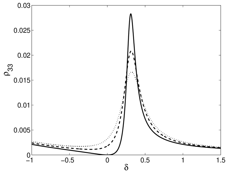
Figure 2: Example fluorescence profiles for a set of values of laser linewidth. The parameter values are (in units where $\Gamma=1$): $\Omega_{1}=0.1$, $\Omega_{2}=1$, $\Delta_{2}=3$, $\Gamma_{1}=\Gamma_{2}=0.5$, and $\gamma=0,0.05,0.1$ for full, dashed, dotted curves, respectively. Note that at finite $\gamma$ the absorption minimum is displaced with respect to $\delta=0$, as remarked by Kofman kofman1997 .

Some example profiles of the 2-photon resonance, as described by equation (12), are shown in figure 2. This illustrates the change in shape of the resonance as $\gamma$ increases.

Although it is useful to have the full expression (12), it is too unwieldy to yield simple insights into the behaviour. We therefore examine it in two limiting cases.

III Resonant lasers

In the situation shown in figure 1a, and such that the lower and upper energy levels in the B manifold are degenerate with states 1 and 3 (respectively) in the D manifold, then in order to optimize the discrimination factor $r$ we choose $\Delta_{1}=\Delta_{2}=0$. There is then a dark resonance in the D manifold, while the B manifold is at a maximum in the fluorescence rate. The absorption in the D manifold is not completely cancelled owing to a non-zero decoherence rate $\gamma$.

For both lasers on resonance with their respective transitions, a factor $(\Omega_{1}^{2}+\Omega_{2}^{2}+4\Gamma_{13}\gamma)$ cancels in the full expression (12) for the excited state population in the D manifold. The expression reduces to

$$\rho_{33}^{\rm D}=\cfrac{2\gamma\Omega_{1}^{2}\Omega_{2}^{2}}{\Omega^{2}Y+2\gamma\left(3\Omega_{1}^{2}\Omega_{2}^{2}+2\Gamma_{13}Y\right)}$$ (13)

where $\Omega^{2}\equiv\Omega_{1}^{2}+\Omega_{2}^{2}$ and $Y\equiv\Gamma_{2}\Omega_{1}^{2}+\Gamma_{1}\Omega_{2}^{2}$.

Assuming the atom–laser coupling constants are such that the Rabi frequency in the B manifold is equal to $C\Omega_{1}$, where $C$ is a constant (such as a Clebsch-Gordan coefficient, for example), and that the excited state in B has the same total decay rate $\Gamma$ as the excited state in D, then the excited state population for the (two level) B manifold is

$$\rho^{\rm B}=\cfrac{1}{2+\Gamma^{2}/C^{2}\Omega_{1}^{2}}\,.$$ (14)

The ratio of steady-state populations is therefore

$$r=\cfrac{\rho^{\rm B}}{\rho_{33}^{\rm D}}=\cfrac{\Omega^{2}Y+2\gamma\left(3\Omega_{1}^{2}\Omega_{2}^{2}+2\Gamma_{13}Y\right)}{2\gamma\Omega_{2}^{2}\left(2\Omega_{1}^{2}+\Gamma^{2}/C^{2}\right)}\,.$$ (15)

This result is valid without restriction—no assumptions have yet been made about the laser intensities or atomic parameters (except those implicit in a master equation treatment in RWA).

In the limit of low probe laser intensity compared to the pump laser intensity, i.e.

$$\Omega_{1}^{2}\ll\Omega_{2}^{2},\;\cfrac{\Gamma_{1}}{\Gamma_{2}}\Omega_{2}^{2}\,,$$ (16)

the ratio is

$$r \approx \cfrac{\Omega_{2}^{2}\Gamma_{1}}{2\gamma\left(2\Omega_{1}^{2}+\Gamma^{2}/C^{2}\right)}$$ (17)

$$\approx \left\{\begin{array}[]{lr}\cfrac{\Omega_{2}^{2}\Gamma_{1}C^{2}}{2\gamma\Gamma^{2}}&,\;\;\;\Omega_{1}^{2}\ll\Gamma^{2},\\ \cfrac{\Omega_{2}^{2}\Gamma_{1}}{4\gamma\Omega_{1}^{2}}&,\;\;\;\Omega_{1}^{2}\gg\Gamma^{2}\,.\end{array}\right.$$ (20)

Hence a large enough pump laser intensity permits very good discrimination to be achieved.

Figure 3 shows the steady state populations in the excited state for the $\left|{I}\right>$ and $\left|{S}\right>$ systems with the pump laser at zero detuning $\Delta_{2}=0$, as a function of the probe laser detuning $\Delta_{1}$. The example parameter values are chosen to illustrate a case where $\left|{I}\right>$ and $\left|{S}\right>$ are adjacent Zeeman sublevels in the atomic ground state at zero magnetic field, and the excited states decay primarily to the ground state; c.f. low-lying levels in alkaline earth ions, as discussed in mcdonnell2003a .

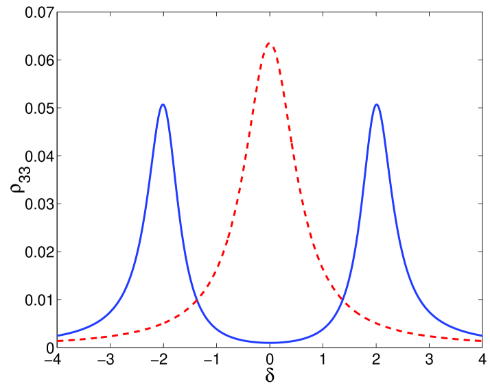
Figure 3: Example of state discrimation for atomic structure of the form shown in figure 1a. The curves show the steady-state value of the excited state population for an atom prepared in $\left|{S}\right>$ (full curve) and $\left|{I}\right>$ (dashed curve), respectively, as a function of detuning $\delta$. The B manifold shows the standard ‘2-level atom’ Lorentzian profile, while the D manifold shows a dark resonance at $\Delta_{1}=0$ in between two peaks at $\pm\Omega_{2}/2$ (these show the positions of the dressed states created by the pump laser). By choosing $\delta=0$ the ratio of excitation rates is maximised. The parameter values for the three level system are (in units where $\Gamma=1$): $\Omega_{1}=0.2$, $\Omega_{2}=4$, $\Gamma_{1}=\Gamma_{2}=0.5$, $\gamma=0.1$. For the two level system $\Omega_{1}=0.2\sqrt{2}$, $\Omega_{2}=0$.

In the case of a ladder system, i.e. when level 2 lies above level 3 in the D manifold, the results are as follows. The OBEs, eq. (2) and (4) are modified so that the spontaneous emission at rate $\Gamma_{2}$ is now from 2 to 3, not the other way around. The steady state solution at zero detuning is

$$\rho_{33}=\frac{2\gamma\Omega_{1}^{2}\Omega_{2}^{2}+\Omega_{1}^{2}\Gamma_{2}\left(\Omega_{1}^{2}+4\Gamma_{23}\gamma\right)}{\Omega^{2}\tilde{Y}-\Gamma_{2}\Omega_{1}^{2}\left(3\Omega_{2}^{2}+2\Gamma_{1}\left(\Gamma_{23}-\Gamma_{13}\right)\right)+2\gamma\left(3\Omega_{1}^{2}\Omega_{2}^{2}+2\Gamma_{13}\tilde{Y}+4\Gamma_{2}\left(\Gamma_{23}-\Gamma_{13}\right)\Omega_{1}^{2}\right)},$$ (21)

where $\tilde{Y}=2\Gamma_{2}\Omega_{1}^{2}+\Gamma_{1}\Omega_{2}^{2}+2\Gamma_{1}\Gamma_{2}\Gamma_{23}$. In the case where the coherence decay rates are purely due to spontaneous emission and laser linewidths, then for the ladder system, equations (9) and (10) should be replaced by

$$\Gamma_{23} = (\Gamma+\Gamma_{2}+\gamma_{2})/2$$ (22)

$$\gamma = (\Gamma_{2}+\gamma_{1}+\gamma_{2})/2.$$ (23)

(In a closed system, $\Gamma=\Gamma_{1}$). In the limit $\Omega_{2}^{2}\gg\Omega_{1}^{2}$ expressions (21) and (13) are the same.

IV Weak probe, large detuning

We next examine the behaviour for a weak probe intensity and large detunings:

$$\Omega_{1}^{2} \ll \frac{\Gamma_{1}}{\Gamma_{2}}\Omega_{2}^{2},\;\Gamma_{1}\alpha\Gamma\,,$$ (24)

$$\Delta_{1}^{2} \gg \alpha^{2}\Gamma^{2},\;\delta^{2}\,.$$ (25)

Under the weak probe condition (24) alone (i.e. without any restriction on detunings), we obtain

$$c_{0} \simeq 16\Omega_{2}^{2}\Gamma_{1}\left[\rule{0.0pt}{10.76385pt}\Delta_{1}^{2}(\delta-\Delta^{\prime})^{2}+\delta^{2}(\alpha\Gamma/2)^{2}\right.$$ (26)

$$\left.+\delta^{2}\Delta_{2}^{2}\frac{\Omega_{1}^{2}}{\Omega_{2}^{2}}\frac{\Gamma_{2}}{\Gamma_{1}}+\frac{\Omega_{2}^{2}\Omega_{1}^{2}}{16}\left(\frac{\Gamma_{2}}{\Gamma_{1}}+2\right)\right]$$

$$c_{1} \simeq 16\Omega_{2}^{2}\Gamma_{1}\left[\frac{\alpha\Gamma\Omega_{2}^{2}}{4}+\frac{\Omega_{1}^{2}}{2\alpha\Gamma\Gamma_{1}}(\Gamma_{1}\Delta_{1}^{2}+\Gamma_{2}\Delta_{2}^{2}\right.$$ (27)

$$\left.+(\Gamma_{1}+\Gamma_{2})\Delta_{1}\Delta_{2})\rule{0.0pt}{10.76385pt}\right]$$

$$c_{2} \simeq 16\Omega_{2}^{2}\Gamma_{1}(\Delta_{1}^{2}+\alpha^{2}\Gamma^{2}/4)$$ (28)

where

$$\Delta^{\prime}\equiv\frac{\Omega_{2}^{2}}{4\Delta_{1}}.$$ (29)

When $\Delta_{1}=\Delta_{2}$, then $\Delta^{\prime}$ is the light shift of the states 2 (upwards when $\Delta_{2}>0$) and 3 (downwards when $\Delta_{2}>0$) caused by the pump laser.

If condition (25) applies, there is a further simplification of the expressions for $c_{i}$, and substituting them into (12) gives

$$\rho_{33}=\frac{\Omega_{\rm eff}^{2}\left(\alpha\left(\frac{\delta^{2}+\gamma^{2}}{2\Delta^{\prime 2}}\right)R+\gamma\right)/2\Gamma_{1}}{(\delta-\Delta^{\prime})^{2}+\left(\frac{\delta\Gamma}{2\Delta_{1}}\right)^{2}\left(\alpha^{2}+\frac{\Gamma_{2}}{\Gamma_{1}}\frac{\Omega_{\rm eff}^{2}}{R^{2}}\right)+\frac{\Omega_{\rm eff}^{2}}{4}\left(\frac{\Gamma_{2}}{\Gamma_{1}}+2\right)+\left(\alpha+\frac{\Omega_{\rm eff}^{2}}{R^{2}}\frac{\Gamma}{\alpha\Gamma_{1}}\right)R\gamma+\gamma^{2}}$$ (30)

where

$$R\equiv\frac{\Omega_{2}^{2}}{4\Delta_{1}^{2}}\Gamma$$ (31)

is (when $\Delta_{1}\simeq\Delta_{2}$) the scattering rate on the strongly driven transition 2–3 per unit population in 2, and

$$\Omega_{\rm eff}\equiv\frac{\Omega_{2}\Omega_{1}}{2\Delta_{1}}$$ (32)

is the effective Rabi frequency for Rabi flopping on the Raman resonance between levels 1 and 2. The reason for introducing $R$ and $\Omega_{\rm eff}$ is that they yield physical insights which will become apparent below.

Many previous treatments of this problem in the limit (24) have assumed the further condition $\Omega_{2}\gg\Omega_{1}\Delta_{1}/\Gamma$, which may usefully be written $R\gg\Omega_{\rm eff}$. It will be important for some of the results to be discussed that we have not made this assumption. A nice feature is that we can find readily understandable physical pictures for this more general case.

The fact that we have not assumed $R\gg\Omega_{\rm eff}$ implies that our results remain valid at large $\Delta_{1}$. For example, away from the 2-photon resonance, i.e. $|\delta|\gg|\Delta^{\prime}|$, the terms proportional to $\delta^{2}$ in (30) dominate, and the result is

$$\rho_{33}\rightarrow\frac{\Omega_{1}^{2}\Gamma/\Gamma_{1}}{4\Delta_{1}^{2}}.$$ (33)

This agrees with the prediction of the rate equations for the three-level system. It can be understood as the excited state population due to single-photon excitation from level 1 by the weaker laser, with the stronger laser playing the role of ‘repumper’.

At small $\Delta_{1},\;\Delta_{2}$ equation (30) remains fairly accurate for small laser linewidth, since the terms which were neglected under assumption (25) are primarily in $c_{1}$ and $c_{2}$, not $c_{0}$.

IV.1 Zero laser linewidth

Let us consider the situation at zero laser linewidth, in order to obtain some physical insights. In this case, $\gamma=0$ and $\alpha=1$. Equation (30) simplifies to

$$\rho_{33}=\frac{\Omega_{1}^{2}\delta^{2}\Gamma/\Gamma_{1}}{4\Delta_{1}^{2}(\delta-\Delta^{\prime})^{2}+\delta^{2}\Gamma^{2}+4\delta^{2}\Delta_{1}^{2}\frac{\Omega_{1}^{2}}{\Omega_{2}^{2}}\frac{\Gamma_{2}}{\Gamma_{1}}+\frac{\Omega_{2}^{2}\Omega_{1}^{2}}{4}\left(\frac{\Gamma_{2}}{\Gamma_{1}}+2\right)}$$ (34)

(We present the equation in terms of $\Omega_{2}$, $\Omega_{1}$ and $\Delta_{1}$ in order to facilitate comparison with previous work stalgies1998 ; leibfried2003 .) This has a zero at $\delta=0$ (the dark resonance) and a peak at $\delta\simeq\Delta^{\prime}$ (the bright resonance). The precise location of the peak is discussed in stalgies1998 .

The denominator of (34) can be simplified to good approximation by replacing the occurrences of $\delta^{2}$ by $\Delta^{\prime 2}$ while retaining the $(\delta-\Delta^{\prime})$ term. This is a good approximation because it is accurate when $\delta=\Delta^{\prime}$, and away from this detuning, the first term in the denominator dominates when $\Delta_{1}$ is large. This substitution gives the canonical ‘Fano’ type of profile Fano1961 :

$$\rho_{33}\simeq\frac{\Omega_{\rm eff}^{2}\left(\delta/\Delta^{\prime}\right)^{2}R/4\Gamma_{1}}{(\delta-\Delta^{\prime})^{2}+R^{2}/4+\Omega_{\rm eff}^{2}\Gamma/2\Gamma_{1}}.$$ (35)

The width of the peak is now easy to extract. The values of $\delta$ at which $\rho_{33}$ is half its maximum value are given by

$$(\delta-\Delta^{\prime})\simeq\frac{f}{2}\left(\frac{f}{\Delta^{\prime}}\pm 1\right).$$ (36)

where

$$f=\left(R^{2}+\Omega_{\rm eff}^{2}\frac{2\Gamma}{\Gamma_{1}}\right)^{1/2}$$ (37)

is the FWHM of the peak and to simplify the RHS we used the condition $f\ll\Delta^{\prime}$ (which follows from (24),(25)).

We next present some physical insights into the behaviour.

IV.1.1 Two models

The main features of $\rho_{33}$ are the zero at dark resonance and the peak at the bright resonance.

As many authors have discussed arimondo1996 ; book:scully , the zero is due to a cancellation between the two excitation routes when the atomic state is $(\Omega_{2}\left|{1}\right>-\Omega_{1}\left|{2}\right>)(\Omega_{1}^{2}+\Omega_{2}^{2})^{-1/2}$ in an interaction picture. When $\delta=0$ this is a stationary state, so once in it the atom does not precess out of it.

To understand the bright resonance, we present two physical models. The first is the well-known ‘dressed atom’ approach; the second is an alternative model based on Rabi flopping and the quantum Zeno effect. For general reviews and references on the quantum Zeno effect, see for example refs misra1977 ; beige1996 ; power1996 ; misra2003 .

The application of the ‘dressed atom’ treatment to EIT and related phenomena has been widely discussed; see arimondo1996 ; book:scully for an introduction and further references. In this model, the behaviour may be regarded as one in which the probe laser excites population from level 1 to a dressed state created by the intense pump laser (see figure 4a). Near the centre of the bright resonance, i.e. when $\delta\simeq\Delta^{\prime}$, eq. (35) takes the form

$$\rho_{33}\simeq\frac{\Omega_{\rm eff}^{2}R/4\Gamma_{1}}{(\delta-\Delta^{\prime})^{2}+R^{2}/4+\Omega_{\rm eff}^{2}\Gamma/2\Gamma_{1}}.$$ (38)

Comparing this with the well-known expression for the upper state population of a two-level atom in steady state, it is seen that the result has a natural interpretation in the dressed atom model. The dressed state has decay rate $R$ and the strength of the coupling to it is $\Omega_{\rm eff}$. The two terms which make up the FWHM (37) of the resonance are then to be interpreted as ‘natural linewidth’ and ‘power broadening’ of the dressed state.

Figure 4: Physical models of the bright resonance. a: The pump laser dresses the atom, the probe laser excites the atom from $\left|{1}\right>$ to the dressed states. These give a broad resonance displaced by $-\Delta^{\prime}$ and a narrow resonance displaced by $\Delta_{2}+\Delta^{\prime}$ from the position of the undressed excited state $\left|{3}\right>$. b: The two lasers together drive Rabi flopping between (undressed) levels $1$ and $2$ by a Raman transition, and the pump laser off-resonantly excites transitions from $\left|{2}\right>$ to $\left|{3}\right>$. The Rabi flopping is resonant when the laser frequencies match the energy difference between 1 and the Stark-shifted level 2.

Our alternative model is based on Rabi flopping and the Zeno effect, as follows (c.f. jong1997 ).

When the difference frequency $\delta$ is tuned to the light shift $\Delta^{\prime}$, the pump and probe lasers drive resonant Rabi flopping between level $1$ and the light-shifted level $2$. Observe that when $\Omega_{2}\gg\Omega_{1}$ and neither of the single-photon transitions are saturated, the population $\rho_{33}$ is produced primarily by excitation from level $2$. The excited state population thus comes about from the combination of the Rabi flopping which moves population between $1$ and $2$, and single-photon excitation from $2$ to $3$ (see figure 4b). However, the single-photon excitation results in a spontaneously emitted photon when $3$ decays, and therefore constitutes a measurement of the atom’s state in the $1$, $2$ basis. This measurement suppresses the Rabi flopping by the quantum Zeno effect. The steady state solution finds a balance between these effects.

This physical picture suggests the following analysis. We take the limit $\Omega_{2}\gg\Omega_{1}$ such that population in 3 is produced purely by excitation from 2 by the pump laser, and treat this by the rate equation

$$\dot{\rho}_{33}=R_{2}\rho_{22}-\Gamma\rho_{33}$$ (39)

where the single-photon excitation rate $R_{2}$ is given by the Fermi Golden Rule: $R_{2}=(\pi/2)\Omega_{2}^{2}g(\Delta_{2})$ where $g$ is a lineshape function. Hence in steady state,

$$\rho_{33}=\frac{R_{2}\rho_{22}}{\Gamma}.$$ (40)

The spontaneous decay of $\rho_{33}$ leads to a Lorentzian lineshape of width $\Gamma$, so in the limit $\Delta_{2}\gg\Gamma,\,\Omega_{2}$,

$$R_{2}\simeq\frac{\Omega_{2}^{2}}{4\Delta_{2}^{2}}\Gamma.$$ (41)

We calculate the steady-state population $\rho_{22}$ by considering the Rabi flopping between levels 1 and 2, and taking $\rho_{22}$ to be the mean population averaged over time. When $R_{2}$ is sufficiently small, and the Raman process is resonant, this Rabi flopping leads to equal average populations $\rho_{11}$ and $\rho_{22}$, i.e. both equal to $1/2$. When $R_{2}$ is non-negligible, on the other hand, the Rabi flopping is interrupted by photon scattering events. These act like measurements, and suppress the flopping by the Zeno effect when they are sufficiently frequent.

An uninterrupted Rabi flopping process would cause the population $\rho_{22}$ to vary with time as:

$$\rho_{22}(t)=\frac{\Omega_{\rm eff}^{2}}{\delta^{\prime 2}+\Omega_{\rm eff}^{2}}\sin^{2}\frac{1}{2}(\Omega_{\rm eff}^{2}+\delta^{\prime 2})^{1/2}t$$ (42)

where $\delta^{\prime}=\delta-\Delta^{\prime}$ is the detuning from the Raman resonance (bright resonance), $\Omega_{\rm eff}$ is given in equation (32), and we assumed the initial condition $\rho_{22}=0$ for convenience (but we expect that the mean population to be calculated will not depend on the initial conditions). The photon scattering acts both as a measurement-type process, collapsing the state to either $1$ or $2$, and also causes optical pumping to $1$. We will treat a simplified case in which we assume the population always goes to $1$ after photon scattering, and then the population in $2$ recommences evolving as (42). This would be the behaviour to be expected when $\Gamma_{1}\gg\Gamma_{2}$. In this case the mean population of 2 is estimated as

$$\bar{\rho}_{22}\simeq\int_{0}^{\infty}P(t)\rho_{22}(t)dt$$ (43)

where $P(t)=R_{2}e^{-R_{2}t}$ is the probability that there is an interval $t$ between scattering events. Performing the integral in (43) we obtain

$$\bar{\rho}_{22}\simeq\frac{1}{2}\frac{\Omega_{\rm eff}^{2}}{\delta^{\prime 2}+R_{2}^{2}+\Omega_{\rm eff}^{2}}$$ (44)

and substituting this in (40) gives

$$\rho_{33}\simeq\frac{\Omega_{\rm eff}^{2}R_{2}/2\Gamma}{\delta^{\prime 2}+R_{2}^{2}+\Omega_{\rm eff}^{2}}$$ (45)

Note the similarity between equations (45) and (38). The Zeno effect calculation reproduces the OBE result when $\Gamma_{1}\simeq\Gamma$, except for factors of 2 associated with $R_{2}$ and $\Omega_{\rm eff}^{2}$. This confirms that it gives a good physical insight into the behaviour. Of course a full quantum Monte-Carlo type of calculation dalibard1992 ; plenio1998 would reproduce the OBE result exactly. The present result simply demonstrates the validity of the ‘Rabi-flopping/Zeno effect’ physical picture.

IV.1.2 Two regimes

The above insights allow us to identify two distinct regimes of behaviour. When $R\gg\Omega_{\rm eff}$, the Zeno effect strongly suppresses the Rabi flopping. In this ‘Zeno regime’,

$$\rho_{33}^{\rm max}=\frac{\Omega_{\rm eff}^{2}}{R\Gamma_{1}}=\frac{\Omega_{1}^{2}}{\Gamma_{1}\Gamma},\;\;\;\;{\rm FWHM}=R$$ (46)

The interpretation in the dressed state picture is that of weak excitation, such that the FWHM is equal to the dressed state’s ‘natural linewidth’ $R$.

When $R^{2}\ll\Omega_{\rm eff}^{2}$ we obtain

$$\rho_{33}^{\rm max}=\frac{R}{2\Gamma},\;\;\;\;{\rm FWHM}=(2\Gamma/\Gamma_{1})^{1/2}\Omega_{\rm eff}.$$ (47)

Here the Rabi flopping leads to $\rho_{11}=\rho_{33}\simeq 1/2$, which leads directly to the value of $\rho_{33}^{\rm max}$, in particular the fact that it depends purely on $R$. The width of the resonance results from the detuning-dependence of the Rabi flopping, and thus is governed purely by $\Omega_{\rm eff}$. In the dressed state picture this is the case where ‘power broadening’ dominates.

IV.2 Finite laser linewidth

We return to equation (30) in order to consider the effect of finite laser linewidth. A useful approximation is the same ‘trick’ as was used for eq. (35) where we replace the $\delta^{2}$ in the denominator by $\Delta^{\prime 2}$. This considerably simplifies the denominator without much loss of accuracy:

$$\rho_{33}\simeq\frac{\Omega_{\rm eff}^{2}\left(\alpha\left(\frac{\delta^{2}+\gamma^{2}}{2\Delta^{\prime 2}}\right)R+\gamma\right)/2\Gamma_{1}}{(\delta-\Delta^{\prime})^{2}+(\alpha R/2+\gamma)^{2}+\Omega_{\rm eff}^{2}(\Gamma/2\Gamma_{1})(1+2\gamma/\alpha R)}$$ (48)

Note that this result is similar to (35) with the substitution $R\rightarrow\alpha R+2\gamma\simeq R+2\gamma$. In other words, the main effect of finite laser linewidth is to increase the ‘linewidth’ term in (35) by $2\gamma$. In the Zeno picture this is an illustration of the fact that measurement-induced collapses have the same effect on a system as phase fluctuations. Their effects add to produce the overall linewidth.

IV.2.1 Effect of laser linewidth on dark resonance

The conditions (24), (25) imply $\Omega_{\rm eff}^{2}\ll\Delta^{\prime 2}$. At $\delta=0$, this can be used to simplify the denominator of (48). If we further assume

$$\gamma\ll\Omega_{2}^{2}/\Gamma$$ (49)

(which is not a severe constraint on the range of validity of the results) then we obtain

$$\rho_{33}^{\rm dark}\simeq\frac{\Omega_{\rm eff}^{2}\gamma/2\Gamma_{1}}{\Delta^{\prime 2}+\Omega_{1}^{2}\gamma/\alpha\Gamma_{1}+\gamma^{2}}$$

$$= \frac{2\Omega_{1}^{2}\gamma/\Gamma_{1}}{\Omega_{2}^{2}+(\Omega_{\rm eff}^{2}/R^{2})(4\Gamma^{2}/\alpha\Gamma_{1})\gamma+(4\Gamma/R)\gamma^{2}}.$$

This result can be interpreted as follows. The dark state is

$$\left|{-}\right>=(\Omega_{2}\left|{1}\right>-\Omega_{1}\left|{2}\right>)(\Omega_{1}^{2}+\Omega_{2}^{2})^{-1/2}.$$ (52)

The combination of $\left|{1}\right>$ and $\left|{2}\right>$ that is orthogonal to this is

$$\left|{+}\right>=(\Omega_{1}\left|{1}\right>+\Omega_{2}\left|{2}\right>)(\Omega_{1}^{2}+\Omega_{2}^{2})^{-1/2}.$$ (53)

Decoherence associated with finite laser linewidth evolves the state towards a random mixture of $\left|{-}\right>$ with the state $\left|{\sim}\right>$ given by

$$\left|{\sim}\right>=(\Omega_{2}\left|{1}\right>+\Omega_{1}\left|{2}\right>)(\Omega_{1}^{2}+\Omega_{2}^{2})^{-1/2}.$$ (54)

A good insight is obtained by analysing the system in the orthonormal basis $\{\left|{3}\right>,\;\left|{-}\right>,\;\left|{+}\right>\}$ (see figure 5). A complete master equation can be obtained in this basis arimondo1996 ; that of course gives exactly the same predictions as those given by the OBEs in their standard form. However, it is noteworthy that the dependence of $\rho_{33}$ on $\gamma$ at the dark resonance point can be obtained to second order in $\gamma$ by a rate equation approach, as follows.

The atom–laser interaction Hamiltonian is $H_{I}=\Omega_{1}\left|{3}\right>\left<{1}\right|+\Omega_{2}\left|{3}\right>\left<{2}\right|$, and the only non-zero matrix element of $H_{I}$ in the chosen basis is $\left<{3}\right|H_{I}\left|{+}\right>=(\Omega_{1}^{2}+\Omega_{2}^{2})^{1/2}$. When $\Omega_{2}^{2}\gg\Omega_{1}^{2}$, the spontaneous decay of $\left|{3}\right>$ to $\left|{-}\right>$ ($\left|{+}\right>$) is at rate approximately $\Gamma_{1}$ ($\Gamma_{2}$) respectively, owing to the relative proportions of $\left|{1}\right>$ and $\left|{2}\right>$ in each of $\left|{-}\right>$ and $\left|{+}\right>$. We model phase decoherence by a spontaneous decay at the rate $\tilde{\Gamma}$ in both directions between $\left|{-}\right>$ and $\left|{+}\right>$. The rate is given by the decay rate $\gamma/2$ between $\left|{-}\right>$ and $\left|{\sim}\right>$, multiplied by the probability that an atom in $\left|{\sim}\right>$ would be found in $\left|{+}\right>$ if measured in the $\left|{\pm}\right>$ basis:

$$\tilde{\Gamma}=\frac{\gamma}{2}\left|\left<\left.{\sim}\right|{+}\right>\right|^{2}=\frac{2\gamma\Omega_{1}^{2}\Omega_{2}^{2}}{(\Omega_{1}^{2}+\Omega_{2}^{2})^{2}}\;\simeq\;2\gamma\Omega_{1}^{2}/\Omega_{2}^{2}\,.$$ (55)

Invoking the limit (25) to simplify the atom-light coupling term, the resulting set of rate equations is

$$\dot{\rho}_{33} = \left(\rho_{++}-\rho_{33}\right)R-\Gamma\rho_{33}$$ (56)

$$\dot{\rho}_{--} = \rho_{33}\Gamma_{1}+\left(\rho_{++}-\rho_{--}\right)\tilde{\Gamma}$$ (57)

$$1 = \rho_{33}+\rho_{--}+\rho_{++}.$$ (58)

Figure 5: Physical model of the effect of decoherence on a dark resonance. The atom is analysed in the basis $\left|{3}\right>$, $\left|{+}\right>$, $\left|{-}\right>$, where $\left|{-}\right>$ is the dark state. A simple rate equation picture, with rates as shown, suffices to give the main features of the behaviour.

The solution is

$$\rho_{33} = \frac{R\tilde{\Gamma}}{R\Gamma_{1}+2(R+\Gamma)\tilde{\Gamma}}$$ (59)

$$\simeq \frac{2\Omega_{1}^{2}\gamma/\Gamma_{1}}{\Omega_{2}^{2}+(\Omega_{\rm eff}^{2}/R^{2})(4\Gamma^{2}/\Gamma_{1})\gamma}$$ (60)

where we used $\tilde{\Gamma}\ll\Gamma_{1}$ which follows from (24). Equation (60) correctly reproduces all the features of (LABEL:dark2) up to second order in $\gamma$. The essence of the dynamics when $\Gamma_{1}\gg R\gg\tilde{\Gamma}$ is that population moves from 3 to the dark state at the rate $\Gamma_{1}$, and from the dark state to 3 (via $\left|{+}\right>$) at the rate $\tilde{\Gamma}$.

Next we consider the overall shape of the 2-photon resonance. The range of values of $\delta$ which interests us is from $0$ to approximately $\Delta^{\prime}$, the position of the bright resonance. Examining (48) we find that when the laser linewidth is sufficient to produce the condition

$$\gamma\gg\alpha R$$ (61)

then the $\gamma$ term in the numerator dominates the other terms. In this case there is no longer a local minimum near $\delta=0$; the dark resonance is completely ‘washed out’. Therefore the condition (61) is sufficient to change the overall lineshape to one close to a Lorentzian function. Note that (61) always occurs at sufficiently large $\Delta_{1}$, independent of the values of the other parameters.

In the case (61) and when also $\gamma\gg\Omega_{\rm eff},\Omega_{\rm eff}^{2}/R$, the complete expression (30) becomes simply a Lorentzian function of linewidth $\gamma$, for $|\delta|\leq|\Delta^{\prime}|$ (and for large $|\delta|$, see eq. (33)).

IV.2.2 Effect of laser linewidth on bright resonance

At the position of the bright resonance ($\delta=\Delta^{\prime}$), the condition (49) is sufficient to make the $\gamma^{2}$ term in the numerator of (48) negligible. In this case (48) gives

$$\rho_{33}^{\rm bright}=\frac{(\Omega_{\rm eff}^{2}/2\Gamma_{1})(\alpha R/2+\gamma)}{(\alpha R/2+\gamma)^{2}+\frac{1}{2}\Omega_{\rm eff}^{2}(\Gamma/\Gamma_{1})(1+2\gamma/\alpha R)}.$$ (62)

In the ‘Zeno regime’ $\Omega_{\rm eff}^{2}\ll R^{2}$ this leads to the simple result

$$\rho_{33}^{\rm bright}\rightarrow\frac{\Omega_{\rm eff}^{2}/2\Gamma_{1}}{\alpha R/2+\gamma}.$$ (63)

V Using the bright resonance for selective excitation

We will now explore the use of the bright resonance as a sharp spectral feature, able to resolve two closely spaced transitions. We have in mind the situation where the atomic structure consists, to good approximation, of two $\Lambda$- systems ‘side by side’ as in fig. 1b. (Similar results can be expected for two ladder-systems). Each of the levels 1,2,3 are split into two closely spaced components (such as Zeeman sublevels, or two rungs of a ladder of vibrational energy levels). We still have just two lasers, and we would like to drive one $\Lambda$- system without driving the other.

The system we want to drive is B and the system we would like not to drive is D. The measure of good discrimination to be adopted is the ratio $r$ between the steady state value for $\rho_{33}$ in the systems or manifolds B and D.

In this section we will discuss the case where the two manifolds have the same coupling constants, so the same Rabi frequencies $\Omega_{2}$, $\Omega_{1}$, but different energy level spacings, such that when the Raman detuning is $\delta$ in system B, it is $\delta-Z$ in system D. The discrimination ratio is then

$$r=\frac{\rho_{33}(\delta)}{\rho_{33}(\delta-Z)}$$ (64)

where $\rho_{33}(\delta)$ is given by (30). The effect of a difference in coupling constants between the two manifolds is discussed in the appendix.

First let us consider the case $\Delta_{1}\gg\Omega_{1},\Omega_{2},\gamma,\Gamma$, which we will refer to for brevity as “$\Delta_{1}\rightarrow\infty$”. This tells us the behaviour of $r$ at large detunings. Equation (30) gives:

$$\rho_{33}(\Delta_{1}\rightarrow\infty)=\frac{\Omega_{\rm eff}^{2}\left(2\alpha\Gamma(\delta^{2}+\gamma^{2})/\Omega_{2}^{2}+\gamma\right)/2\Gamma_{1}}{(\delta-\Delta^{\prime})^{2}+\gamma\Omega_{1}^{2}/\alpha\Gamma_{1}+\gamma^{2}}.$$ (65)

At large $\Delta_{1}$, the light shift is small compared to $Z$, so to produce the discrimination factor $r$ the dark resonance is irrelevant. We tune system B to bright resonance, and it is found that $r$ is maximised when $\Omega_{1}^{2}\ll\gamma\Gamma\ll\Omega_{2}^{2}$. In this case, using (65) and (64),

$$r(\Delta_{1}\rightarrow\infty)=\frac{Z^{2}+\gamma^{2}}{\left(2\alpha\Gamma Z^{2}/\Omega_{2}^{2}+\gamma\right)\gamma}.$$ (66)

Next let us consider the case where we arrange that $\Delta^{\prime}=Z$. This means that when the B system is tuned to bright resonance, the D system is simultaneously tuned to dark resonance, and we expect a large value for $r$. Examining the ratio $r=\rho_{33}^{\rm bright}/\rho_{33}^{\rm dark}$ given by equations (62) and (IV.2.1), it is found that $r$ is maximised in the ‘Zeno regime’ $\Omega_{\rm eff}^{2}\ll R^{2}$. It is always possible to enter this regime without affecting the light shift by reducing $\Omega_{1}$ at fixed values of $\Omega_{2}$ and $\Delta_{1}$. From (63) and (IV.2.1) we then obtain

$$r(\Delta^{\prime}=Z)=\frac{Z^{2}+\gamma^{2}}{(\alpha R/2+\gamma)\gamma}.$$ (67)

To maximise $r$, one should reduce $R$ as much as possible, subject to the constraint $\Delta^{\prime}=Z$. This means that, for given $Z$, the value of $R$ is limited by the available laser power: $R=4Z^{2}\Gamma/\Omega_{2}^{2}$, so

$$r(\Delta^{\prime}=Z)=\frac{Z^{2}+\gamma^{2}}{(2\alpha\Gamma Z^{2}/\Omega_{2}^{2}+\gamma)\gamma}.$$ (68)

This is the same result as (66). Therefore if $\Omega_{1}$ is reduced sufficiently to enter the Zeno regime, then for laser linewidths satisfying $\gamma\ll\Omega_{2}^{2}/\Gamma$, the value of $r$ is the same at $\Delta_{1}=\Omega_{2}^{2}/4Z$ (where the D system is tuned to dark resonance) as when $\Delta_{1}\rightarrow\infty$.

V.1 Discussion

The ratio $r=\rho_{33}(\delta)/\rho_{33}(\delta-Z)$ is plotted in figure 6 as a function of pump laser parameters $\Omega_{2}$, $\Delta_{2}$, for the example case of $Z=0.2\Gamma$, $\gamma=0.001\Gamma$ and small $\Omega_{1}$. The ridge observed in the surface corresponds to the condition $\Delta^{\prime}=Z$, with a slight offset owing to the displacement of the absorption minimum remarked in the caption to figure 2 (see below). Each line of $r$ at constant $\Omega_{2}$ has a local maximum at the ridge, and then tends to this same maximum $r$ at large $\Delta_{2}$. This is the basic behaviour predicted by equations (66) and (68). A wider numerical exploration indicated that the value given by (66) and (68) is always close to the maximum $r$ when $\gamma$ is small enough to allow good discrimination ($r\gg 1$).

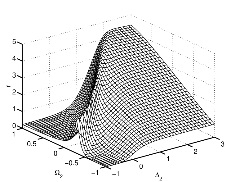
Figure 6: Discrimination ratio $r$ for the case of two $\Lambda-$systems with the same coupling constants, and 2-photon resonance conditions of frequency separation $Z$. The surface shows $r$ as a function of $\Delta_{2}$ and $\Omega_{2}$ for the case $Z=0.2$, $\gamma=0.001$, and small $\Omega_{1}$, in units where $\Gamma=1$. All scales are logarithmic, marked in powers of 10. Note that the range of validity of the approximate equation (30) is such that it gives the same results (i.e. no discernible difference in this surface plot) as the exact equation (12), even where $\Delta_{1}$ is small.

Equations (66) and (68) are among the central results of this paper. We had expected that arranging the special case where the light-shift $\Delta^{\prime}$ matches the offset $Z$ would provide an especially good discrimination, as quantified by the ratio $r$. However, although we find that this case does provide the maximum $r$ at given $Z$, $\gamma$ and $\Omega_{2}$, we find that the same value of $r$ is also available when $\Delta^{\prime}\neq Z$ by using a large detuning. Therefore the EIT can be useful to increase the rate of signal acquisition, but it does not provide an improved discrimination of the two resonances in the atom. Hence the title of this paper is a misnomer for the case considered here: the most important feature is the presence of the bright resonance, not the dark resonance. This could be called quantum state discrimination by ‘EIO’, that is, electromagnetically-induced opacity.

At small $\Omega_{2}$ and $\gamma$, $r$ increases as $\Omega_{2}^{2}$ and does not depend on $Z$, while at large $\Omega_{2}$ it saturates to $r\rightarrow Z^{2}/\gamma^{2}+1$. The latter result is exactly the same as equation (1) for single-photon excitation limited by laser linewidth, if for given $Z$ we compare the summed laser linewidths in the 2-photon case with the single laser linewidth in the single-photon case. This is owing to the Fano lineshape becoming Lorentzian when the laser linewidth dominates its FWHM. The surprising feature is that choosing laser parameters in order to get a non-Lorentzian Fano profile, with its apparently useful sub-Lorentzian behaviour near $\delta=0$, in fact can only make matters worse at given laser linewidth and intensity.

Close inspection of the numerical results reveals a further detail. This is that for a strong pump beam, the optimal detuning is larger than that which leads to $\Delta^{\prime}=Z$, and a slightly increased $r$ is available. This is owing to the fact that for finite $\gamma$ the minimum absorption is displaced from $\delta=0$, as shown in figure 2. We find that this offset is given by $2\gamma\Delta_{1}/(\alpha\Gamma+4\gamma)$, in agreement with kofman1997 . An increase in $\Delta_{1}$ reduces the light shift and hence allows the D manifold to be closer to the minimum when the B manifold is at the peak.

To summarize, in the case of two $\Lambda$-systems of the same coupling constant but different energy level separations, we find that the highest value of $r$ is obtained both at $\Delta^{\prime}=Z$, and at large $\Delta_{2}$. Going to large $\Delta_{2}$ has the disadvantage that the rates get small, so the system is more sensitive to drifts and other line-broadening mechanisms. Therefore the optimum conditions are, for given $Z$, $\gamma$:

$$\Omega_{2}$$ as large as possible (69)

$$\Delta_{2} = \frac{\Omega_{2}^{2}}{4Z}\left(1+\frac{\gamma\Omega_{2}^{2}}{2\Gamma Z^{2}}\right)-Z$$ (70)

$$\Omega_{1} \ll \max\left(\frac{Z\Gamma}{\Omega_{2}},\;\frac{\Delta\gamma}{\Omega_{2}}\right)$$ (71)

where in (70) we have included an adjustment for the displaced minimum, and the condition (71) is to avoid power-broadening of the bright resonance. Equation (68) shows also that smaller laser linewidth is always advantageous to increase $r$, whereas $r$ saturates as a function of $Z$, ceasing to increase significantly with $Z$ once $Z$ is large compared to $\Omega_{2}(\gamma/2\Gamma)^{1/2}$.

These conclusions are valid when the laser linewidth is caused by, or is equivalent to, phase diffusion. If other sources of noise, such as jitter and drift, dominate (with a non-Lorentzian frequency distribution) then the evaluation of $r$ has to be reconsidered. In some circumstances it is appropriate to take average values of $\rho_{33}^{\rm dark}$ and $\rho_{33}^{\rm bright}$, using equations (62) and (IV.2.1) averaged over the relevant laser frequency distribution. In certain cases the dark resonance can allow a much greater discrimination than would be obtained using narrow single-photon transitions driven by lasers with the same frequency distribution.

VI Laser cooling of a trapped atom

Laser cooling of a trapped 3-level atom using narrow two-photon resonances has been discussed by various authors, see ref. lindberg1986 ; marzoli1994 and references therein for a general discussion. We will examine the specific case of using the bright resonance (and accompanying dark resonance) for continuous cooling; this was considered by lindberg1986 ; marzoli1994 ; reiss1996 ; reiss2002 ; morigi2000 ; morigi2003 .

Using the formulation as given by lindberg1986 , we obtain the steady state solution for the motional density matrix $\rho_{m}$ of a trapped atom or ion in the Lamb-Dicke limit. Expanding the master equation to lowest order in the Lamb-Dicke parameters $\eta_{1},\eta_{2}$ (associated with the laser excitation on transitions $1\leftrightarrow 3$, $2\leftrightarrow 3$ respectively), the solution is found to be a thermal state $\rho_{m}=\sum(1-q)q^{n}\left|{n}\right>\left<{n}\right|$ where $q=A_{+}/A_{-}$ is the ratio of heating- to cooling-rate coefficients. The rate coefficients $A_{\pm}$ are given by

$$A_{\pm} = \left(\Gamma_{1}\alpha_{1}\eta_{1}^{2}+\Gamma_{2}\alpha_{2}\eta_{2}^{2}\right)\rho_{33}$$ (72)

$$+\mbox{Re}\left\{\mbox{ Tr}\left[2V(L_{0}\pm i\nu)^{-1}V\rho\right]\right\}$$

where $\alpha_{1},\alpha_{2}$ are coefficients describing the angular distribution of spontaneously emitted photons (e.g. $\alpha=1/3$ for isotropic emission), $\rho_{33}$ is the internal upper state population in steady state with motional effects ignored, i.e. as given by (12), $V$ is the internal-state part of the laser–atom interaction which corresponds to first sideband excitation:

$$V=\eta_{1}\frac{\Omega_{1}}{2}(\left|{3}\right>\left<{1}\right|-\left|{1}\right>\left<{3}\right|)+\eta_{2}\frac{\Omega_{2}}{2}(\left|{3}\right>\left<{2}\right|-\left|{2}\right>\left<{3}\right|),$$

and $L_{0}$ is the zeroth order Liouville operator acting on the internal state, defined such that the master equation $\dot{\rho}=L_{0}(\rho)$ gives precisely the OBEs for the semi-classical treatment of a free atom, as given in (2)–(7).

This situation may be compared with the selective excitation which is the main subject of this paper. Let $\omega_{z}$ be the vibrational frequency of the given atom in the (assumed harmonic) trap. Efficient cooling, and low steady-state temperature, is obtained when the cooling rate $A_{-}$ is high and the heating rate $A_{+}$ is low. This requires strong excitation of the first red sideband at $\omega_{0}-\omega_{z}$ while avoiding excitation of the carrier and the first blue sideband, at $\omega_{0}$ and $\omega_{0}+\omega_{z}$ respectively, where $\omega_{0}$ is the centre of some resonance feature in the excitation spectrum of a free atom—in our case, the bright resonance. The energy level structure is akin to that of fig. 1b rather than 1a, since the ladder of vibrational energy levels leads to an infinite set of $\Lambda$-systems. To obtain an enhancement from EIT, the lasers should be blue detuned, i.e. $\Delta_{1},\Delta_{2}>0$. The frequency difference $Z$ considered in section V corresponds to the vibrational energy $\omega_{z}$. The selectivity parameter $r$ discussed in section V corresponds to $1/q$. Just as we suspected that we might observe large selectivity $r$ when $Z=\Delta^{\prime}$, we now investigate whether we observe an especially low $q$ when $\omega_{z}=\Delta^{\prime}$.

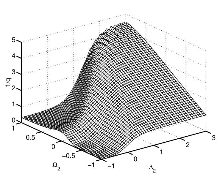
Figure 7: Cooling/heating ratio $1/q$ for the case of laser cooling of a trapped three-level atom using the bright resonance. The surface shows $1/q$ as a function of $\Delta_{2}$ and $\Omega_{2}$ for the case $\omega_{z}=0.2$, $\gamma=0.001$, and small $\Omega_{1}$, $\eta_{1}$, $\eta_{2}$, in units where $\Gamma=1$. All scales are logarithmic, marked in powers of 10. (The small irregular ripples at large $1/q$ are a numerical artifact.)

Figure 7 shows $1/q$ for the case of laser cooling, for the same parameters as were chosen in figure 6 for the case of $r$ and selective excitation. The two sets of results are broadly similar. The main difference is that the ridge (i.e. high value of $1/q$, giving low temperature) produced by the ‘EIT condition’ $\omega_{z}=\Delta^{\prime}$ is now lower and broader, compared to the ridge in $r$ in fig. 6. This is because we now have many $\Lambda$ systems, and the heating coefficient $A_{+}$ is produced both by the carrier and the blue sideband excitation: the dark resonance can suppress one or other of these, but not both. As a result, the lines of $1/q$ at constant $\Omega_{2}$ show no local maximum as a function of $\Delta_{2}$. $q$ (and hence the steady-state temperature) falls monotonically as a function of pump laser detuning.

Although the EIT condition does not produce the lowest steady-state temperature $T_{0}$, for given values of pump laser intensity and trap frequency, it can be useful for other reasons. For example it was shown in morigi2000 that it produces a high ratio $A_{-}/T_{0}$ of cooling rate to steady-state temperature, and permits cooling of motion in all directions to the same $T_{0}$.

VII Appendix

Here we present the solution of the OBEs for a 3-level $\Lambda$-type system.

The solution for $\rho_{13}$ can be extracted by a standard matrix inversion method, see for example book:scully , where the case $\Delta_{2}=0$ is treated in full. We are interested here in $\rho_{33}$ so we present this quantity.

The solution for $\gamma=0$ has been presented by various authors, see for example janik1985 whose notation is close to ours. The solution for general $\gamma$ was discussed in brewer1975 ; lindberg1986 and is closely related to the ladder system discussed in whitley1976 . However the expressions in these works are even more lengthy and obscure than those given below; we require the simplest form possible.

In order to simplify the expressions without much loss of generality, we assume $\Gamma_{13}=\Gamma_{23}$ (this is valid when the lasers’ linewidths are equal, and approximately valid when they are unequal but small compared to $\Gamma$).

In this case, the steady state value of $\rho_{33}$ is as given in (12), with the coefficients in the denominator as follows:

$$c_{0} = (\Omega_{1}^{2}+\Omega_{2}^{2})^{2}Y+16\delta^{2}\Gamma_{13}^{2}Y$$ (73)

$$+4\delta^{2}\Omega_{1}^{2}\Omega_{2}^{2}(6\Gamma_{13}-(\Gamma_{1}+\Gamma_{2}))$$

$$+16\delta^{2}(\Gamma_{2}\Omega_{1}^{2}\Delta_{2}^{2}+\Gamma_{1}\Omega_{2}^{2}\Delta_{1}^{2})$$

$$-8\delta(\Delta_{1}\Gamma_{1}\Omega_{2}^{4}-\Delta_{2}\Gamma_{2}\Omega_{1}^{4})$$

where $Y\equiv\Gamma_{2}\Omega_{1}^{2}+\Gamma_{1}\Omega_{2}^{2}$,

$$c_{1}=2\left(\Omega_{1}^{2}+\Omega_{2}^{2}\right)\left(4\Gamma_{13}Y+3\Omega_{1}^{2}\Omega_{2}^{2}\right)$$

$$+4\frac{\Omega_{1}^{2}\Omega_{2}^{2}}{\Gamma_{13}}\left(\Gamma_{1}\Delta_{1}^{2}+\Gamma_{2}\Delta_{2}^{2}+(\Gamma_{1}+\Gamma_{2})\Delta_{1}\Delta_{2}\right),$$

and

$$c_{2} = 8\left[2\Gamma_{13}^{2}Y+3\Gamma_{13}\Omega_{1}^{2}\Omega_{2}^{2}\right.$$ (75)

$$\left.+2\left(\Delta_{2}^{2}\Gamma_{2}\Omega_{1}^{2}+\Delta_{1}^{2}\Gamma_{1}\Omega_{2}^{2}\right)\right].$$

Equation (73) can also be written:

$$c_{0} = 16\Omega_{2}^{2}\Gamma_{1}\Delta_{1}^{2}\left(\delta-\frac{\Omega_{2}^{2}}{4\Delta_{1}}\right)^{2}$$ (76)

$$+16\Omega_{1}^{2}\Gamma_{2}\Delta_{2}^{2}\left(\delta-\frac{\Omega_{1}^{2}}{4\Delta_{2}}\right)^{2}$$

$$+16\delta^{2}\Gamma_{13}^{2}Y+4\delta^{2}\Omega_{1}^{2}\Omega_{2}^{2}(6\Gamma_{13}-(\Gamma_{1}+\Gamma_{2}))$$

$$+\Omega_{1}^{2}\Omega_{2}^{2}\left(Y+\left(\Omega_{1}^{2}+\Omega_{2}^{2}\right)(\Gamma_{1}+\Gamma_{2})\right).$$

This form is useful in order to clarify where the resonances are, and to derive equation (26).

VII.1 Degenerate $\Lambda$-systems

Here we briefly discuss the case of two degenerate $\Lambda$-systems, but where discrimination is still possible because of a difference in coupling constants.

We adapt the notation so that now the parameters $\Omega_{i}$ refer to manifold D, and we define $C_{i}=\Omega_{i}^{\rm B}/\Omega_{i}$, $i=1,2$ where $\Omega_{i}^{\rm B}$ are the Rabi frequencies in manifold B. The maximum $r$ occurs either when system B is tuned to bright resonance, or when system D is tuned to dark resonance. The latter case is only relevant when $\gamma$ is very small, and then $r$ is a ratio of two very small excitation rates. We will concentrate on the case where $\gamma$ is somewhat larger, and then it is best to tune B to bright resonance. We then have $r=\rho_{33}^{\rm B}/\rho_{33}^{\rm D}$ where $\rho_{33}^{\rm B}$ is given by equation (63):

$$\rho_{33}^{\rm B}=\frac{C_{1}^{2}C_{2}^{2}\Omega_{\rm eff}^{2}/2\Gamma_{1}C_{1}^{2}}{\alpha C_{2}^{2}R/2+\gamma}.$$ (77)

The symbols $\Omega_{\rm eff}$, $R$ refer to their values in system D, and we assume the decay rate $\Gamma_{1}$ is enhanced in system B, compared to D, by $C_{1}^{2}$. We have also assumed the Zeno regime in order to avoid power-broadening.

The situation in manifold D is given by equation (48) at $\delta=\Delta^{\prime}_{\rm B}-\Delta^{\prime}_{\rm D}=(C_{2}^{2}-1)\Delta^{\prime}$, hence:

$$\rho_{33}^{\rm D}=\frac{\Omega_{\rm eff}^{2}(\alpha RC_{2}^{4}/2+\gamma)/2\Gamma_{1}}{(C_{2}^{2}-1)\Delta^{\prime 2}+(\alpha R/2+\gamma)^{2}},$$ (78)

where we assumed (49). The largest values of $r$ are obtained at high detuning, such that $R\ll\gamma$, where we find

$$r(\Delta_{1}\rightarrow\infty)=\left(C_{2}(C_{2}-1)\Delta^{\prime}\right)^{2}/\gamma^{2}+1.$$ (79)

References

- [1] E. Arimondo. Coherent population trapping in laser spectroscopy. In E. Wolf, editor, Progress in optics, volume XXXV, pages 257–354. North-Holland, 1996.
- [2] M.O. Scully and M.S. Zubairy. Quantum Optics. Cambridge University Press, 1997.
- [3] M. Fleischhauer and M.O. Scully. Quantum sensitivity limits of an optical magnetometer based on atomic phase coherence. Phys. Rev. A, 49:1973–1986, 1994.
- [4] M. Fleischhauer, T. McIllrath, and M.O. Scully. Coherent population trapping and Fano-type interferences in lasing wothout inversion. Appl. Phys. B, 60:S123–S127, 1995.
- [5] A. Aspect, E. Arimondo, R. Kaiser, N. Vansteenkiste, and C. Cohen-Tannoudji. Laser cooling below the one-photon recoil energy by velocity-selective coherent population trapping. Phys. Rev. Lett., 61:826–829, 1988.
- [6] M. Lindberg and J. Javanainen. Temperature of a laser-cooled trapped three-level ion. J. Opt. Soc. Am. B, 3:1008–1017, 1986.
- [7] G. Morigi, J. Eschner, and C.H. Keitel. Ground state laser cooling using electromagnetically induced transparency. Phys. Rev. Lett., 85:4458–4461, 2000.
- [8] J. Gea-Banacloche, Y-Q. Li, S-Z. Jin, and M. Xiao. Electromagnetically induced transparency in ladder-type inhomogeneously broadened media: theory and experiment. Phys. Rev. A, 51:576–584, 1995.
- [9] M. McDonnell, J.-P. Stacey, S. C. Webster, J. P. Home, A. Ramos, D. M. Lucas, D. N. Stacey, and A. M. Steane. Single-atom spin measurement without dipole moment. 2003. Submitted.
- [10] I. Marzoli, J. I. Cirac, R. Blatt, and P. Zoller. Laser cooling of trapped three-level ions: Designing two-level systems for sideband cooling. Phys. Rev. A, 49:2771–2779, 1994.
- [11] D. Reiß, K. Abich, W. Neuhauser, Ch. Wunderlich, and P. E. Toschek. Raman cooling and heating of two trapped Ba+ ions. Phys. Rev. A, 65:053401, 2002.
- [12] Y. Stalgies, I. Siemers, B. Appasamy, and P.E. Toschek. Light shift and Fano resonances in a single cold ion. J. Opt. Soc. Am. B, 15:2505–2514, 1998.
- [13] R.M. Whitley and C.R. Stroud, Jr. Double optical resonance. Phys. Rev. A, 14:1498–1513, 1976.
- [14] A.G. Kofman. Electromagnetically induced transparency with coherent and stochastic fields. Phys. Rev. A, 56:2280–2291, 1997.
- [15] D. Leibfried, R. Blatt, C. Monroe, and D. Wineland. Quantum dynamics of single trapped ions. Rev. Mod. Phys., 75:281–324, 2003.
- [16] U. Fano. Effects of configuration interaction on intensities and phase shifts. Physical Review, 124:1866–, 1961.
- [17] B. Misra and E. Sudershan. The Zeno’s paradox in quantum theory. J. Math. Phys., 18:756–763, 1977.
- [18] A. Beige and G.C. Hegerfeldt. Projection postulate and atomic quantum Zeno effect. Phys. Rev. A, pages 53–65, 1996.
- [19] W.L. Power and P.L. Knight. Stochastic simulations of the quantum Zeno effect. Phys. Rev. A, 53:1052–1059, 1996.
- [20] B Misra and I Antoniou. Quantum Zeno effect. In Proc. 22nd Solvay Conf. Physi.: The Physics of Communication, 2003. at press.
- [21] F.B. de Jong, R.J.C. Spreeuw, and H.B. van Linden van den Heuvell. Quantum Zeno effect and V-scheme lasing without inversion. Phys. Rev. A, 55:3918–3922, 1997.
- [22] J. Dalibard, Y. Castin, and K. Mølmer. Wave-function approach to dissipative processes in quantum optics. Phys. Rev. Lett., 68:580–583, 1992.
- [23] M.B. Plenio and P.L. Knight. The quantum-jump approach to dissipative dynamics in quantum optics. Rev. Mod. Phys., 70:101–144, 1998.
- [24] D. Reiß, A. Lindner, and R. Blatt. Cooling of trapped multilevel ions: A numerical analysis. Phys. Rev. A, 54:5133–5140, 1996.
- [25] G. Morigi. Cooling atomic motion with quantum interference. Phys. Rev. A, 67:033402, 2003.
- [26] G. Janik, W. Nagourney, and H. Dehmelt. Doppler-free optical spectroscopy on the Ba+ mono-ion oscillator. J. Opt. Soc. Am. B, 2:1251–1257, 1985.
- [27] R.G. Brewer and E.L. Hahn. Coherent two-photon processes: Transient and steady-state cases. Phys. Rev. A, 11:1641–1649, 1975.